Multilinear Representations of Rotation Groups within

Geometric Algebra

M. A. J. Ashdown, S. S. Somaroo

y

, S. F. Gull, C. J. L. Doran and A. N. Lasenby.

MRAO, Cavendish Laboratory, Madingley Road, Cambridge CB3 0HE, U.K..

26th November 1997

Abstract

It is shown that higher-weighted representations of rotation groups can be con-

structed using multilinear functions in geometric algebra. Methods for obtaining

the irreducible representations are found, and applied to the spatial rotation group,

S

O

(3), and the proper Lorentz group,

S

O

+

(1 3). It is also shown that the repres-

entations can be generalised to non-linear functions, with applications to relativistic

wave equations describing higher-spin particles, such as the Rarita-Schwinger equa-

tions. The internal spin degrees of freedom and the external spacetime degrees of

freedom are handled within the same mathematical structure.

PACS: 02.10.Sp 02.20.Sv 03.65.Fd 03.65.Pm.

1 Introduction

The vector and spinor representations of rotation groups are well known. In this paper

we show that it is possible to extend these to higher-weighted representations by using

multilinear functions of vector variables. Our representations are constructed using the

language of geometric algebra, an introduction to which is given in the following subsec-

tion.

First we show how to construct the representations of an arbitrary rotation group

SO

+

(p q) and demonstrate the methods for nding their irreducible components. The

most important method is monogenic decomposition 1], which can be rened by consider-

ing the symmetry between the arguments of the function. A monogenic function belongs

to the null space of the vector derivative (the Dirac operator). Analysis of the monogenic

properties of functions forms an important part of Cliord analysis.

We use these methods to nd the irreducible representations of the rotation group of

Euclidean 3-space SO(3) and the proper Lorentz group SO

+

(1 3). In both cases we show

how to nd all the integral- and half-integral-spin representations of the groups. These

are useful in constructing wave equations describing higher-spin particles.

In the last section we examine the Dirac equation and its generalisations to higher-spin

wave equations, such as the Rarita-Schwinger equations. We show that the multilinear

representations can be extended to encompass non-linear functions, and these can be used

to construct the wavefunctions. This provides a unied method for describing the internal

and external degrees of freedom of a higher-spin particle. In using geometric algebra we

are able to overcome one of the deciencies in the matrix formulation of linear algebra,

Email: [e-mail]

y

Current Address: BCMP, Harvard Medical School, 240 Longwood Ave., Boston, MA 02115, USA.

1

that it is not easily able to relate linear and non-linear methods. Polynomial projection 1]

enables us to immediately construct the non-linear functions which form the basis of the

spacetime part of the wavefunction from the multilinear functions derived earlier for the

spin part of the wavefunction.

1.1 Geometric Algebra

Geometric algebra is based upon Cliord algebra with emphasis on the geometric inter-

pretation of elements of the algebra rather than their matrix representations. Here we

present a brief introduction to geometric algebra and the conventions that are used in this

paper. More comprehensive introductions can be found in Hestenes and Sobczyk 2] and

Gull, Lasenby and Doran 3].

Geometric algebra is a graded algebra in which the fundamental product is the geo-

metric product. Vectors, which have grade 1, will be written in lower case Roman letters

(a,b,

etc.

). The geometric product of vectors ab can be split into its symmetric and anti-

symmetric parts

ab = a b + a

^

b

(1)

where

a b

1

2

(ab + ba)

a

^

b

1

2

(ab

;

ba)

(2)

The inner product a b is scalar-valued (grade 0). The outer product a

^

b represents a

directed plane segment produced by sweeping a along b. This new element is called a

bivector and has grade 2. By introducing more vectors, higher-grade elements can be

constructed, trivectors (grade-3) a

^

b

^

c represent volumes, and so on, up to the dimension

of the space under consideration. A grade-r element of the algebra is called an r-vector

and a general element of the geometric algebra, possibly consisting of many grades, is

called a multivector. If we multiply an r-vector A

r

by an s-vector B

s

the geometric

product can be expanded as follows

A

r

B

s

=

h

A

r

B

s

i

r

+

s

+

h

A

r

B

s

i

r

+

s

;2

+ :::+

h

A

r

B

s

i

j

r

;

s

j

(3)

where

h

C

i

t

denotes projecting out the grade-t elements of C. The notation for inner and

outer products is retained for the lowest and highest grade elements in this expansion,

A

r

^

B

s

h

A

r

B

s

i

r

+

s

A

r

B

s

h

A

r

B

s

i

j

r

;

s

j

:

(4)

We use the convention that inner and outer products take precedence over geometric

products in expressions.

In addition we dene the commutator product, which is equal to half the commutator

bracket

A

B =

1

2

(AB

;

BA) =

1

2

A B]:

(5)

Reversion is the operation by which the order of vectors in a geometric product is reversed,

it is dened by

g

AB = ~B ~A

(6)

where a vector reverses to give itself, ~a = a.

Although geometric algebra can be constructed in an entirely basis-free form, in many

applications it is useful to introduce a set of basis vectors. The geometric algebra with

2

signature (p q) which will be denoted as

G

p q

has n = p + q orthonormal basis vectors,

e

i

i = 1 ::: n which obey

e

i

e

j

=

8

>

>

>

<

>

>

>

:

1 i = j = 1 ::: p

;

1 i = j = p + 1 ::: p + q

0 i

6

= j

(7)

The grade-r space in this algebra is denoted

G

rp q

.

The highest-grade element that can be formed from this basis has grade n and is called

the pseudoscalar. It is dened by

I

e

1

^

e

2

^

:::

^

e

n

= e

1

e

2

:::e

n

:

(8)

All grade-n elements must be a scalar multiple of the pseudoscalar.

This paper makes use of some results of geometric calculus, which is based on the

vector derivative. If we write a vector in terms of its components, a = a

i

e

i

, then the

vector derivative with respect to a is dened as

@

a

e

i

@

@a

i

(9)

where the reciprocal vectors are dened by

e

i

(

;

1)

i

;1

(e

1

^

:::

^

e

i

^

:::

^

e

n

)I

;1

(10)

and the check on e

i

denotes that it is omitted from the product. The vector derivative,

besides being an operator, also inherits the properties of a vector from a. The vector

derivative with respect to position x is given the symbol

r

,

r

@

x

:

(11)

This paper uses the properties of multilinear functions which are functions in geometric

algebra that are linear in all of their arguments. A function

M(a

1

::: a

k

)

(12)

which takes values in any part of the geometric algebra and is linear in its k vector

arguments will be called k-linear.

There are two geometric algebras, the Pauli algebra and the spacetime algebra, which

for reasons of convention have their own notation.

1.2 The Pauli Algebra

The Pauli algebra

G

3

0

is the geometric algebra of three dimensional Euclidean space. The

three basis vectors are

1

,

2

and

3

, which satisfy

j

k

=

jk

:

(13)

The pseudoscalar of the algebra is

i

1

2

3

:

(14)

The algebra has eight basis elements

1

f

k

g

f

i

k

g

i

1 scalar 3 vectors 3 bivectors 1 pseudoscalar

grade 0 grade 1

grade 2

grade 3

(15)

3

1.3 The Spacetime Algebra

The spacetime algebra (STA) is the geometric algebra of Minkowski spacetime,

G

1

3

. The

basis vectors are

0

,

1

,

2

and

3

, which satisfy

=

= diag(+

;

;;

):

(16)

We also dene the bivectors,

k

=

k

0

(k = 1 2 3)

(17)

and the pseudoscalar,

i =

0

1

2

3

=

1

2

3

:

(18)

These denitions are compatible with those for the Pauli algebra given above, because

the Pauli algebra is a sub-algebra of the STA. The STA has 16 basis elements,

1

f

g

f

k

i

k

g

f

i

g

i

1 scalar 4 vectors 6 bivectors 4 trivectors 1 pseudoscalar

grade 0 grade 1

grade 2

grade 3

grade 4

(19)

Vectors in the STA have a projective relation to those in the Pauli algebra,

a

0

= a

0

+

a

(20)

where a

0

= a

0

and

a

= a

^

0

. The bivector

a

in the STA corresponds to the vector in

the Pauli algebra relative to the frame dened by the unit timelike vector

0

.

2 Representations of Rotation Groups

In this section we shall develop the formalism we need to describe higher-weighted rep-

resentations of the rotation group SO

+

(p q) and nd its irreducible representations.

2.1 The Representations

Any rotation belonging to the group SO

+

(p q) leaves the inner product of two vectors

in the geometric algebra

G

p q

unchanged. Such a rotation is described by a rotor R, an

even-graded element of the algebra which satises

R ~R = 1:

(21)

Rotors are used to dene the two types of representation of the the rotation group. The

one-sided representations, which will be denoted as ^U

R

, in which the rotor acts one-sidedly

on a multivector ,

^U

R

] = R

(22)

and the two-sided representations, which will be denoted as ^V

R

, in which the rotor R acts

two-sidedly on a multivector M,

^V

R

M] = RM ~R:

(23)

4

The group Spin

+

(p q) of which the one-sided representations are members is a double

covering of the group SO

+

(p q). This follows from the fact that in the two-sided rep-

resentations, the rotation represented by a rotor R could equally well be represented by

;

R,

^V

(;

R

)

= ^V

R

but this does not hold for the one-sided representations.

We extend the carrier spaces of these two types of representations to multilinear func-

tions of vector variables by dening their actions on k-linear functions to be

^U

R

(a

1

::: a

k

)] = R( ~Ra

1

R ::: ~Ra

k

R)

(24)

^V

R

M(a

1

::: a

k

)] = RM( ~Ra

1

R ::: ~Ra

k

R) ~R:

(25)

Most rotors can be written in the form

R = exp

;

1

2

C

(26)

where C is a bivector. If C is a simple bivector then it denes the plane in which the

rotation occurs. The algebra of the bivectors

G

2

p q

, which is closed under the commutator

product (5), is equivalent to the Lie algebra so(p q) of the rotation group 4].

By writing the operator ^U

R

in a form similar to (26) we can dene the linear operator

^L

C

which corresponds to C,

^U

R

exp

1

2

^L

C

:

(27)

Take for example a linear function (a) which transforms under ^U

R

. In order to nd the

action of ^L

C

on (a) we write C = B, where is a scalar and use (26) to substitute for

R,

^U

R

(a)] = exp

1

2

^L

B

(a) = e

1

2

B

(e

;

1

2

B

ae

1

2

B

):

(28)

Dierentiating with respect to and setting = 0, we nd that

1

2

^L

B

(a) =

1

2

B(a) + (a B):

(29)

The factors of

1

2

in this equation arise naturally from the denition of the rotor (26). The

set of operators ^L

B

form a representation of the Lie algebra which obeys the commutation

relation

^L

B

^L

C

] = ^L

B C

]

(30)

or writing the same expression using the commutator product,

^L

B

^L

C

= ^L

B

C

:

(31)

The geometric algebra

G

p q

has

1

2

n(n

;

1) linearly-independent bivectors, thus SO(p q)

has

1

2

n(n

;

1) generators.

Extending ^L

B

to act on functions with k arguments is straightforward

1

2

^L

B

(:::)] =

1

2

B(:::) +

k

X

i

=1

(::: a

i

B :::)

(32)

each argument makes a contribution of one term to the expression. A similar procedure

gives the action of ^L

B

on functions which transform two-sidedly,

1

2

^L

B

M(:::)] = B

M(:::) +

k

X

i

=1

M(::: a

i

B :::):

(33)

5

2.2 Invariant Subspaces

We must nd the irreducible representations of the rotation group. To this end we now

seek the invariant subspaces of the representations.

The simplest kind of invariant subspace is one in which elements have a denite sym-

metry among their arguments. An operator ^T

ij

can be dened which exchanges the ith

and jth arguments of a function,

^T

ij

(::: a

i

::: a

j

:::) = (::: a

j

::: a

i

:::)

(34)

which is used to construct operators which symmetrise or antisymmetrise between the ith

and jth arguments of a function.

^S

ij

1

2

(1 + ^T

ij

)

^A

ij

1

2

(1

;

^T

ij

):

(35)

These operators commute with the action of the group, so if a function has symmetric or

antisymmetric arguments, the action of the group does not change this property. Com-

binations of ^S

ij

and ^A

ij

can be constructed to represent all distinct symmetries between

the arguments of a k-linear function. A general product of these operators will be denoted

as ^Y. It can be shown that there is a one-to-one correspondence between these functions

and the order-k Young tableaux.

A two-sided representation preserves the grade of an object which it transforms. This

property can be shown by considering the action of ^V

R

on an r-vector A

r

= a

1

^

a

2

^

:::

^

a

r

where a

1

a

2

::: a

r

are vectors. Since R ~R = 1,

^V

R

A

r

] = RA

r

~R = (Ra

1

~R)

^

(Ra

2

~R)

^

:::

^

(Ra

r

~R)

(36)

which is also be an r-vector, so ^V

R

preserves the grades of all r-vectors, formally,

^V

R

G

rp q

] =

G

rp q

:

(37)

A one-sided representation does not preserve the grade of an object, however, since

rotors are even-graded elements of the algebra, this representation separates the space of

multivectors into even and odd grades, formally,

^U

R

G

+

p q

] =

G

+

p q

^U

R

G

;

p q

] =

G

;

p q

:

(38)

We shall call an one-sided irreducible representation a spinor representation. A spinor

representation can also accommodate an ideal structure. A spinor or spinor-valued func-

tion can be multiplied on the right by an idempotent element of the algebra E = E

2

to

project it into a right ideal of the algebra,

= E:

(39)

The ideal structure is preserved by the action of ^U

R

since the rotor acts only on the left.

Another property that is not changed by the action of the group is that of monogenicity.

If a function

M

(a

1

::: a

k

) is monogenic, it has the property

@

a

j

M

(a

1

::: a

k

) = 0

(40)

6

for all j = 1 2 ::: k. This property is unchanged by the action of a rotor. Take, for

example, a function which transforms under ^U

R

@

a

j

^U

R

M

(a

1

::: a

k

)] = @

a

j

R

M

(a

0

1

::: a

0

k

)

(41)

where a

0

j

= ~Ra

j

R. Using the chain rule to rearrange the transformed function,

@

a

j

R

M

(a

0

1

::: a

0

k

) = @

a

j

( ~Ra

j

R) @

a

0

j

R

M

(a

0

1

::: a

0

k

)

= R@

a

0

j

M

(a

0

1

::: a

0

k

):

(42)

Thus, under the action of ^U

R

, the monogenic properties of a function are not changed,

^U

R

@

a

j

M

(a

1

::: a

k

)] = R@

a

0

j

M

(a

0

1

::: a

0

k

):

(43)

A similar argument applies to the double-sided transformation (25). From this, it can be

shown that monogenicity is also preserved under the action of elements of the Lie algebra.

We shall denote any monogenic function by the primary label

M

.

The grade-invariance property of the two-sided transformation and monogenic invari-

ance do not dene mutually exclusive invariant subspaces and so cannot be used simul-

taneously to nd the irreducible representations. We conclude that the irreducible rep-

resentations of rotation groups consist of basis functions which have distinct symmetry

among their arguments. For functions which transform one-sidedly, they correspond to

particular terms in the monogenic decomposition and possibly have an ideal structure or,

for functions which transform two-sidedly, they possess denite grade.

2.3 Monogenic decomposition

In the last section we proved that the monogenic properties of a function are not changed

by the action of the rotation group or its Lie algebra. Arbitrary k-linear functions can

be decomposed into monogenic and non-monogenic parts in a similar manner to Taylor

decomposition of functions in one dimension.

An inner product can be dened between two k-linear functions, and ,

h

j

i

=

h

(@

a

1

::: @

a

k

)~(a

1

::: a

k

)

i

(44)

which is invariant under the action of both types of representation of the rotation group. A

complex structure can always be added to this inner product. The functions are orthogonal

if

h

j

i

= 0. For simplicity it will be assumed that at least one of the functions is not null.

A function (a

1

::: a

k

) can be decomposed into a monogenic part and a part orthogonal

to it:

(a

1

::: a

k

) =

M

(a

1

::: a

k

) + M(a

1

::: a

k

)

(45)

where

M(a

1

::: a

k

) = a

1

1

(a

2

::: a

k

) + a

2

2

(a

1

a

3

::: a

k

) + :::

+a

k

k

(a

1

::: a

k

;1

):

(46)

The fact that each term in M is orthogonal to

M

follows easily from the denition of the

inner product, since for any function (a

1

::: a

j

;1

a

j

+1

::: a

k

) which does not depend

on a

j

,

h

a

j

(a

1

::: a

j

;1

a

j

+1

::: a

k

)

jM

(a

1

::: a

k

)

i

=

(a

1

::: a

j

;1

a

j

+1

::: a

k

)

j

@

a

j

M

(a

1

::: a

k

)

= 0

(47)

7

by the monogenic properties of

M

. Recursive use of the partial decomposition produces

the complete monogenic decomposition

(a

1

::: a

k

) =

k

X

l

=0

M

l

(a

1

::: a

k

)

(48)

where

M

0

(a

1

::: a

k

) =

M

(a

1

::: a

k

)

M

l

(a

1

::: a

k

) =

P

a

(1)

:::a

(

l

)

M

(a

(

l

+1)

::: a

(

k

)

)

(49)

where the sum runs over all permutations of the numbers 1 ::: k. The decomposition

is unique and the M

l

are orthogonal

h

M

j

j

M

l

i

= 0 for j

6

= l:

(50)

Under the action of ^U

R

, the function M

l

transforms as

^U

R

M

l

(a

1

::: a

k

)] =

X

a

(1)

::: a

(

l

)

^U

R

M

(a

(

l

+1)

::: a

(

k

)

)]

(51)

similarly for ^V

R

. This shows that only the monogenic part of the function is transformed,

the polynomial of vectors remaining unchanged.

We conclude that any arbitrary k-linear function can be constructed out of monogenic

functions as in (48).

The symmetry between the arguments can be used to rene the monogenic decompos-

ition,

(a

1

::: a

k

) =

k

X

l

=0

X

^

Y

^YM

l

(a

1

::: a

k

)

(52)

where M

l

is dened as before (49) and the decomposition is summed over all possible

symmetries among the arguments, ^Y. This is known as the Fischer decomposition 1].

3 Representations of SO(3)

In this section we will investigate the multilinear representations of the rotation group of

Euclidean space, SO(3).

3.1 Generators and Eigenstates

The Pauli algebra

G

3

0

has three linearly-independent bivectors, i

1

, i

2

and i

3

, so SO(3)

has three generators, for which the following notation is introduced.

^J

k

1

2

^L

i

k

(53)

for k = 1 2 3. Since i

2

k

=

;

1 these are compact generators. The

f

^J

k

g

obey the com-

mutation relation

^J

k

^J

l

] =

;

klm

^J

m

:

(54)

This relation diers from the usual convention because the generators are related to the

bivectors of the Pauli algebra, rather than the vectors as in more conventional treatments.

The representations will be classied as eigenstates of the generators. To do this we

need to introduce a complex structure, but rather than using the scalar imaginary we shall

8

use an operation within the real geometric algebra to play the same role. The geometric

operation that we choose will be denoted by ^|.

The spin of a particle is described by two quantum numbers which give the total spin

and the spin in a particular plane. The `total spin' operator is the Casimir operator of

the group,

^

J

2

^J

1

2

+ ^J

2

2

+ ^J

3

2

:

(55)

Denoting this as the square of a vector is somewhat misleading, but we shall retain this

notation for the sake of convention. One of the generators must be chosen to complete

our commuting set of operators. The conventional choice is ^J

3

which measures the spin in

the i

3

plane. The states are described in terms of the eigenstates of these two operators,

the eigenvalues of which are s and m respectively. Acting on an abstract state

j

sm

i

,

^

J

2

j

sm

i

=

;

s(s + 1)

j

sm

i

(56)

^J

3

j

sm

i

= ^|m

j

sm

i

:

(57)

The raising and lowering operators are the same as in conventional treatments,

^J

= ^J

1

^|^J

2

:

(58)

The spin-s irreducible representation will be referred to as D(s). Products of the repres-

entations obey the familiar Clebsch-Gordon decomposition,

D(s

1

)

D(s

2

)

D(s

1

+ s

2

)

:::

D(

j

s

1

;

s

2

j

):

(59)

3.2 The Spin-

1

2

Representation

The spin-

1

2

representation is the fundamental spinor representation which could take val-

ues in the even or odd sectors of the algebra. It is more convenient to let spinor take

values in the even sub-algebra

G

+

3

0

, of which the basis elements are

f

1 i

1

i

2

i

3

g

:

(60)

Translating the conventional representation into geometric algebra 5, 6] it is found that

the spin-

1

2

representation is complexied by right-multiplication by i

3

^|

i

3

:

(61)

The even sub-algebra is closed under this operation.

Using the raising and lowering operators (58) the spin-up and spin-down basis states

are found to be

+

= 1

;

= i

1

:

(62)

Coecients of these states are dened over the `complex' eld,

f

1 ^|

g

so a general state

takes values over the whole even sub-algebra. The convention for the basis states used here

diers slightly from those of Doran

etal.

6] since we have adopted a dierent convention

for the generators.

9

3.3 The Spin-1 Representation

The vector space of the Pauli algebra

G

1

3

0

has three basis vectors which could form a basis

for the spin-1 representation D(1). We cannot use the same complexication operation

as the spin-

1

2

representation here, but we note that the space of bivectors

G

2

3

0

could also

form a suitable basis for D(1). So to complexify this representation we employ an

ad

hoc

construction: the pseudoscalar i =

1

2

3

, which has a negative square, is used to

complexify the representation,

^|A

iA:

(63)

A consequence of this is that the D(1) representation is vector- and bivector-valued and has

3 complex or 6 real degrees of freedom. The complexication operations we have dened

for the spin-

1

2

and the spin-1 representations at rst sight appear to be incompatible, but

later we shall show that they can be reconciled.

Using the raising and lowering operators the three basis states A

sm

can be constructed.

A

1

1

=

1

p

2

(

1

+ i

2

)

A

1

0

=

;

i

3

A

1

;1

=

1

p

2

(

1

;

i

2

)

(64)

the coecients of which take values over the `complex' eld

f

1 ^|

g

.

3.4 Relating Spin-

1

2

and Spin-

1

Representations

Here we shall attempt to relate the spin-

1

2

representations to the spin-1 representations

and reconcile the diering complexication operators. This process will be very useful

later in constructing higher-spin representations.

We can attempt to construct a spin-1 state from two spin-

1

2

states,

1

and

2

, in the

form

M =

1

; ~

2

(65)

where ; is a xed multivector to be determined. If the spinors are transformed under ^U

R

we nd that,

1

; ~

2

R

7;

!

^U

R

1

];^U

R

~

2

] = R

1

;(R

2

)~ = R

1

; ~

2

~R = ^V

R

1

; ~

2

]

(66)

so M transforms like an integral-spin representation. Taking the product of the repres-

entations, M will transform as

D(

1

2

)

D(

1

2

) = D(1)

D(0):

(67)

Since ; is a multivector, M will take values in all possible grades of the algebra. The

scalar and pseudoscalar parts can be identied with the spin-0 representation, since these

grades are invariant under rotation,

=

D

1

; ~

2

E

0

3

(68)

and the vector and bivector parts are identied with the spin-1 representation as in the

previous section,

A =

D

1

; ~

2

E

1

2

:

(69)

10

Inserting the spin-

1

2

basis states into (69), we nd that ; is

;

(1 +

3

)

1

:

(70)

The presence of the idempotent

1

2

(1+

3

) in ; ensures that the diering complexication

operators dened earlier are consistent.

3.5 Half-Integral-Spin Representations

To nd a general half-integral-spin representation, we will be looking for spinor-valued

functions which transform under ^U

R

. The complexication operator for these functions

is the same as that for the spinor representation.

Consider a spinor-valued linear function, (a), which transforms under ^U

R

. The

monogenic decomposition (48) can be used to analyse the transformation properties of

the function,

(a) =

M

(a) + a

(71)

where

M

(a) is the monogenic part of the function, and the second term is the residual

component which is dened by

=

1

3

@

a

(a)

(72)

which will take values in the odd-graded part of the algebra

G

;

3

0

. This function will

transform as the

D(

1

2

)

D(1) = D(

3

2

)

D(

1

2

)

(73)

representation. Under the action of ^U

R

, (a) transforms to

R( ~RaR) = R

M

( ~RaR) + aR:

(74)

It can be seen that the second term transforms with one rotor like the spin-

1

2

representa-

tion, so the monogenic part of the function can be identied with the spin-

3

2

representation.

To construct the higher-spin representations we will need some `complex'-valued func-

tions of a vector variable from which to construct the contributions of the arguments,

1

(a) =

1

p

2

(a

1

+ a

2

^|)

0

(a) =

;

a

3

^|

;1

(a) =

1

p

2

(a

1

;

a

2

^|):

(75)

These are closely related to the spin-1 basis states. They have been written using ^|since

they will be useful in constructing both integral and half-integral-spin states.

The spin-

3

2

multiplet can be constructed from these functions and the spin-

1

2

basis

states

(62),

3

2

3

2

(a) =

+

1

(a)

3

2

1

2

(a) =

1

p

3

(

;

1

(a) +

p

2

+

0

(a))

3

2

;

1

2

(a) =

1

p

3

(

+

;1

(a) +

p

2

;

0

(a))

3

2

;

3

2

(a) =

;

;1

(a):

(76)

These four basis states are monogenic functions. The associated spin-

1

2

doublet consists

of the residual functions from the monogenic decomposition,

1

2

1

2

(a) =

1

p

3

(

p

2

;

1

(a)

;

+

0

(a)) =

1

p

3

ai

1

2

;

1

2

(a) =

1

p

3

(

;

p

2

+

;1

(a) +

;

0

(a)) =

;

1

p

3

a

1

:

(77)

11

These functions are orthonormal under the functional inner product (44).

Now consider a spinor-valued bilinear function, (a b), which will transform under ^U

R

as

D(

1

2

)

D(1)

D(1) = D(

5

2

)

2D(

3

2

)

2D(

1

2

)

(78)

The monogenic decomposition of (a b) is

(a b) =

M

(a b) + a

M

0

(b) + b

M

00

(a) + ab

1

+ ba

2

(79)

The symmetry between the arguments need not be taken into account since there can-

not be any antisymmetric monogenic functions in

G

3

0

. If there were such a monogenic

M

A

(a b), it could be written as a function of a bivector

M

A

(a

^

b). By linearity,

@

a

M

A

(a

^

b) = @

a

(a

^

b) @

B

M

A

(B) = 0

(80)

where the chain rule has been applied. Expanding B over the bivector basis elements,

this becomes

b i

1

M

A

(i

1

) + b i

2

M

A

(i

2

) + b i

3

M

A

(i

3

) = 0

(81)

which must hold for all values of b. It is easy to show that this implies that each of

the components of

M

A

(a

^

b) vanishes. It follows that in 3 dimensions a k-linear mono-

genic cannot be antisymmetric in any two of its arguments, it therefore must be totally

symmetric.

Under the action of ^U

R

, (a b) transforms to

R( ~RaR ~RbR) = R

M

( ~RaR ~RbR) + aR

M

0

( ~RbR)

+bR

M

00

( ~RaR) + abR

1

+ baR

2

(82)

Again it can be seen that it is the monogenic part which behaves as the irreducible

representation with the highest spin, in this case spin-

5

2

. There are also two spin-

3

2

and

two spin-

1

2

representations, as predicted in (78). The m =

5

2

state will be

5

2

5

2

(a b) =

+

1

(a)

1

(b)

(83)

and the remaining basis states of the D(

5

2

) representation can be constructed using the

lowering operator.

The properties of a function which corresponds to a general half-integral-spin irredu-

cible representation can now be deduced. Consider a spinor-valued k-linear function

(a

1

::: a

k

)

(84)

which transforms under ^U

R

as

D(

1

2

)

D(1)

:::

D(1)

|

{z

}

k times

= D(k +

1

2

)

D(k

;

1

2

)

:::

D(

1

2

):

(85)

The monogenic part of this function

M

(a

1

::: a

k

)

(86)

which must be totally symmetric, will correspond to the D(k +

1

2

) irreducible representa-

tion. The m = k +

1

2

basis state will be

k

+

1

2

k

+

1

2

(a

1

::: a

k

) =

+

1

(a

1

):::

1

(a

k

):

(87)

The rest of the spin-(k +

1

2

) basis states can be constructed from this using the lowering

operator.

12

3.6 Integral-Spin Representations

In the same way as we constructed the spin-1 representation from the spin-

1

2

repres-

entation, we can construct any integral-spin representation from the half-integral-spin

representations deduced above. A linear function which transforms under ^V

R

can be

constructed from a spinor-valued linear function

1

(a) and a spinor

2

.

M(a) =

1

(a); ~

2

(88)

where ; = (1 +

3

)

1

as before (70). M(a) will be multivector-valued, and it will belong

to the

D(

1

2

)

D(1)

D(

1

2

)

(89)

representation. If

1

(a) is restricted to be monogenic

M

(a), then the function

M

0

(a) =

M

(a); ~

2

(90)

belongs to the

D(

3

2

)

D(

1

2

) = D(2)

D(1)

(91)

representation. This can be restricted further by selecting the vector and bivector part

A(a) =

hM

(a); ~

2

i

1

2

:

(92)

which will transform as the D(2) irreducible representation. The scalar and pseudoscalar

part of M

0

(a) will transform as D(1). Inserting the D(

3

2

) and D(

1

2

) basis states from (62)

and (76) the basis states of the D(2) irreducible representation are

A

2

2

(a) = A

1

1

(a)

A

2

1

(a) =

1

p

2

(A

1

0

(a) + A

0

1

(a))

A

2

0

(a) =

1

p

6

(A

1

;1

(a) + A

;1

1

(a) + 2A

0

0

(a))

A

2

;1

(a) =

1

p

2

(A

;1

0

(a) + A

0

;1

(a))

A

2

;2

(a) = A

;1

;1

(a):

(93)

where A

1

, A

0

and A

;1

are shorthand for the m = 1, m = 0 and m =

;

1 basis states of

the D(1) representation respectively.

This procedure can now be generalised to nd the properties of a function which corres-

ponds to any integral-spin irreducible representation. Consider a k-linear function which

transforms under ^V

R

, constructed from a k-linear spinor-valued function

1

(a

1

::: a

k

)

and a spinor

2

,

M(a

1

::: a

k

) =

1

(a

1

::: a

k

); ~

2

:

(94)

It will transform as

D(

1

2

)

D(1)

:::

D(1)

|

{z

}

k times

D(

1

2

) = D(k + 1)

D(k)

:::

D(0)

(95)

If

1

(a

1

::: a

k

) is restricted to be a monogenic then the function

M

0

(a) =

M

(a

1

::: a

k

); ~

2

(96)

will transform as the

D(k +

1

2

)

D(

1

2

) = D(k + 1)

D(k)

(97)

13

representation. Again if this is restricted to the vector and bivector parts, the resulting

function

A(a

1

::: a

k

) =

hM

(a

1

::: a

k

); ~

2

i

1

2

(98)

corresponds to the D(k + 1) irreducible representation.

We have now identied the functions which correspond to all of the irreducible repres-

entations of SO(3) and in the process discovered many monogenic functions in the Pauli

algebra.

4 Representations of the Lorentz Group

We now turn our attention the the proper Lorentz group SO

+

(1 3). The representations

we nd in this section will be useful in describing relativistic wave equations.

4.1 Generators

The spacetime algebra has six linearly-independent bivectors,

f

k

i

k

g

, therefore the

Lorentz group has six generators, for which we introduce the following shorthand notation,

^J

k

=

1

2

^L

i

k

^K

k

=

1

2

^L

k

(99)

where k = 1 2 3. These operators obey the commutation relations

^J

i

^J

j

] =

;

ijk

^J

k

^K

i

^K

j

] =

ijk

^J

k

^J

i

^K

j

] =

ijk

^K

k

:

(100)

The

f

^J

k

g

form a closed sub-algebra, which is identical to the Lie algebra of SO(3) in the

previous section. Again these relations dier slightly from conventional treatments.

4.2 Classication of Irreducible Representations

We shall introduce complex structure to the Lorentz group within the real STA, using

the operator ^|to stand for the complexication operation and deducing its action on the

representations. The complex structure can be used to dene two sets of generators from

the generators of the Lorentz group 7]

^A

k

=

1

2

(^J

k

+ ^|^K

k

) ^B

k

=

1

2

(^J

k

;

^|^K

k

)

(101)

where k = 1 2 3. These operators have the following commutation relations

^A

k

^A

l

] =

;

klm

^A

m

^B

k

^B

l

] =

;

klm

^B

m

^A

k

^B

l

] = 0:

(102)

The operators form two uncoupled sets of generators which individually behave like the

generators of SO(3). The group generated by these uncoupled operators will therefore

behave as a direct product of two copies of SO(3). If s

a

is the spin of the ^A

k

irreducible

representation and s

b

is the spin of the ^B

k

irreducible representation then their direct

product space, which can be described by a pair of spin weights (s

a

s

b

), will have (2s

a

+

1)(2s

b

+ 1) complex degrees of freedom. An eigenstate will be equivalent to the product

of two SO(3) eigenstates

j

s

a

s

b

m

a

m

b

i

=

j

s

a

m

a

i

j

s

b

m

b

i

:

(103)

14

The operators

^

A

2

= ^A

1

2

+ ^A

2

2

+ ^A

3

2

(104)

^

B

2

= ^B

1

2

+ ^B

2

2

+ ^B

3

2

(105)

are the Casimir operators of the group, where the `vector' notation has again been used.

These can be written in terms of the ^J

k

and ^K

k

operators by taking the sum and dierence,

^

A

2

+ ^

B

2

=

1

2

(^

J

2

;

^

K

2

)

(106)

^

A

2

;

^

B

2

=

;

^|^

J

^

K

:

(107)

It will be found that a particular irreducible representation can be distinguished from

other representations with the same s = s

a

+ s

b

by its grade or algebraic properties. We

shall refer to all such representations as spin-s representations, for example,

;

1

2

1

2

and

(1 0)

(0 1) are both spin-1 representations.

Because the representations have a direct product structure, the Lorentz group ana-

logue of the Clebsh-Gordon decomposition is quite simple,

(s

a

1

s

b

1

)

(s

a

2

s

b

2

) =

X

s

a

s

b

(s

a

s

b

)

(108)

where the sum runs independently over the values

s

a

= s

a

1

+ s

a

2

s

a

1

+ s

a

2

;

1 :::

j

s

a

1

;

s

a

2

j

s

b

= s

b

1

+ s

b

2

s

b

1

+ s

b

2

;

1 :::

j

s

b

1

;

s

b

2

j

:

(109)

Now we have identied the irreducible representations, we can classify their basis

states. The basis states will be expressed as eigenstates of the operators ^J

3

and ^K

3

with

eigenvalues m and n respectively, because these are related to simple bivector generators.

These states will still be eigenstates of ^A

3

and ^B

3

, the eigenvalues are related by

m = m

a

+ m

b

(110)

n = m

a

;

m

b

:

(111)

The basis states are thus characterised by four spin quantum numbers, s

a

, s

b

, m and n.

Operating on an eigenstate

j

s

a

s

b

mn

i

we nd

^

A

2

j

s

a

s

b

mn

i

=

;

s

a

(s

a

+ 1)

j

s

a

s

b

mn

i

(112)

^

B

2

j

s

a

s

b

mn

i

=

;

s

b

(s

b

+ 1)

j

s

a

s

b

mn

i

(113)

^J

3

j

s

a

s

b

mn

i

= ^|m

j

s

a

s

b

mn

i

(114)

^K

3

j

s

a

s

b

mn

i

= n

j

s

a

s

b

mn

i

(115)

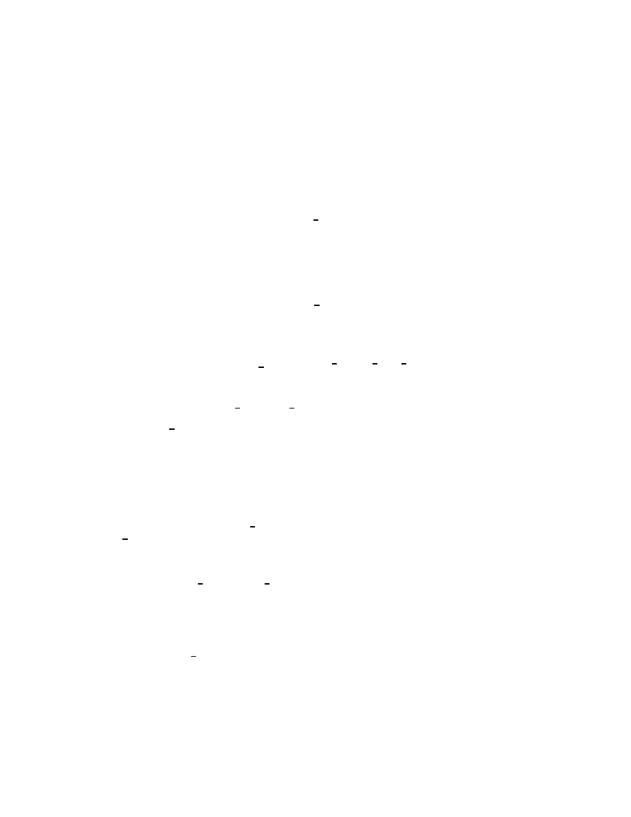
The raising and lowering operators

^A

= ^A

1

^|^A

2

^B

= ^B

1

^|^B

2

(116)

which raise and lower the m

a

and m

b

quantum numbers respectively can be used to move

between the basis states of the representation, which is show in terms of the m and n

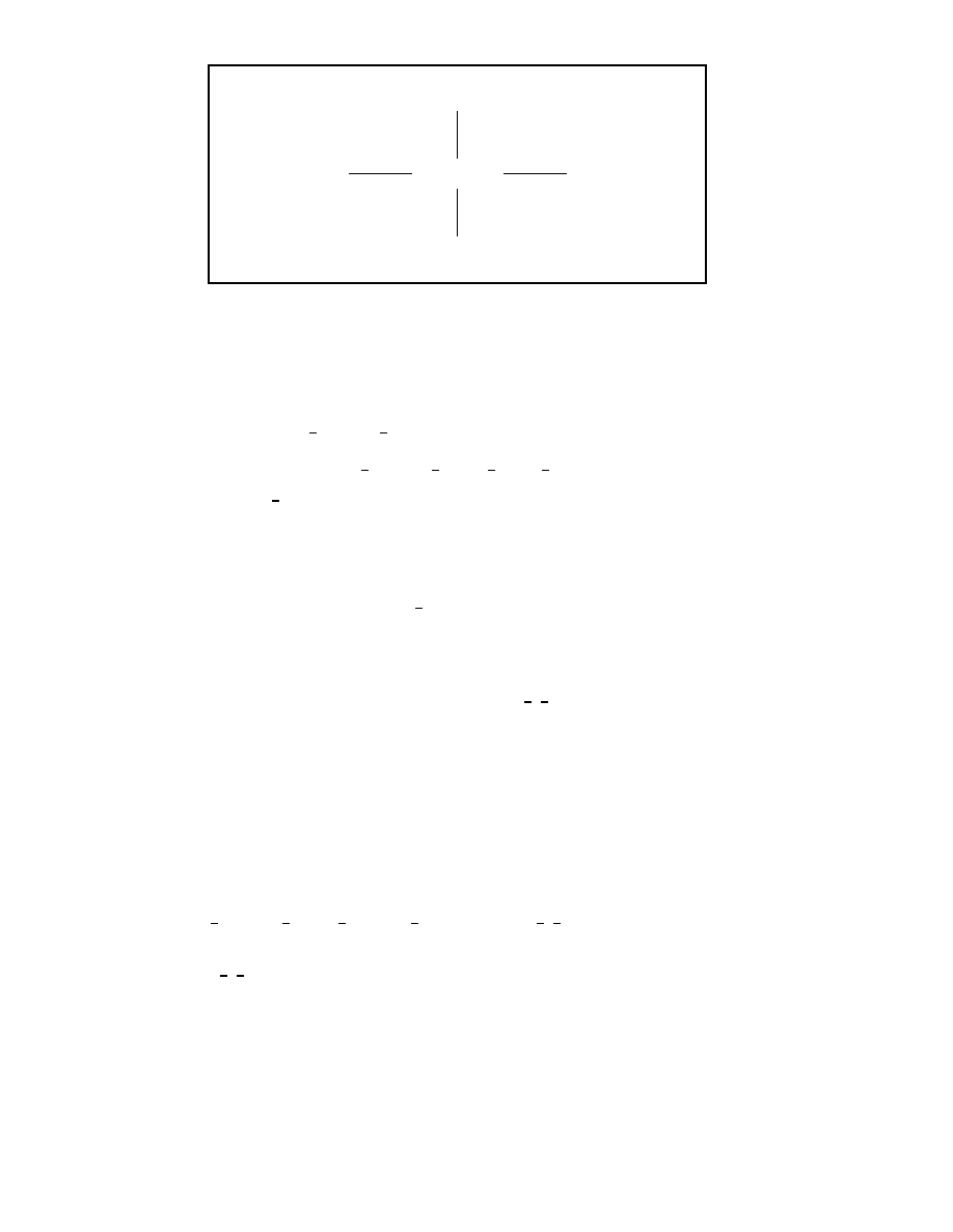
states in Figure 1.

15

j

s

a

s

b

m n

i

j

s

a

s

b

m + 1 n + 1

i

j

s

a

s

b

m + 1 n

;

1

i

j

s

a

s

b

m

;

1 n + 1

i

j

s

a

s

b

m

;

1 n

;

1

i

;

;

;

@

@

@

R

@

@

@

I

;

;

;

^A

+

^A

;

^B

+

^B

;

Figure 1: Raising and Lowering Operators for Spin-s Irreducible Representation of the

Lorentz Group.

An alternative, incomplete method of classifying the irreducible representations of

the Lorentz group is to decompose them into representations of the subgroup SO(3), as

eigenstates of ^

J

2

. The (s

a

s

b

) representation contains the

D(s

a

)

D(s

b

) = D(s

a

+ s

b

)

:::

D(

j

s

a

;

s

b

j

)

(117)

representations of SO(3) and the (s

a

s

b

)

(s

b

s

a

) representation will contain two copies

of each of these subgroup representations. The operator ^J

3

will be used to nd the

eigenstates of these subgroup representations. The alternative quantum numbers which

corresponds to the eigenstates of ^

J

2

and ^J

3

are j and m,

(^

J

2

;

^

K

2

)

j

s

a

s

b

jm

i

=

;

2(s

a

(s

a

+ 1) + s

b

(s

b

+ 1))

j

s

a

s

b

jm

i

(118)

^

J

2

j

s

a

s

b

jm

i

=

;

j(j + 1)

j

s

a

s

b

jm

i

(119)

^J

3

j

s

a

s

b

jm

i

= ^|m

j

s

a

s

b

jm

i

(120)

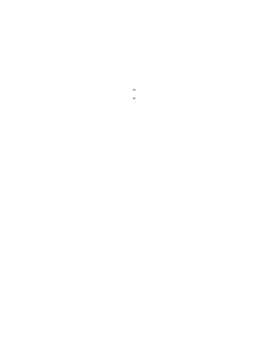
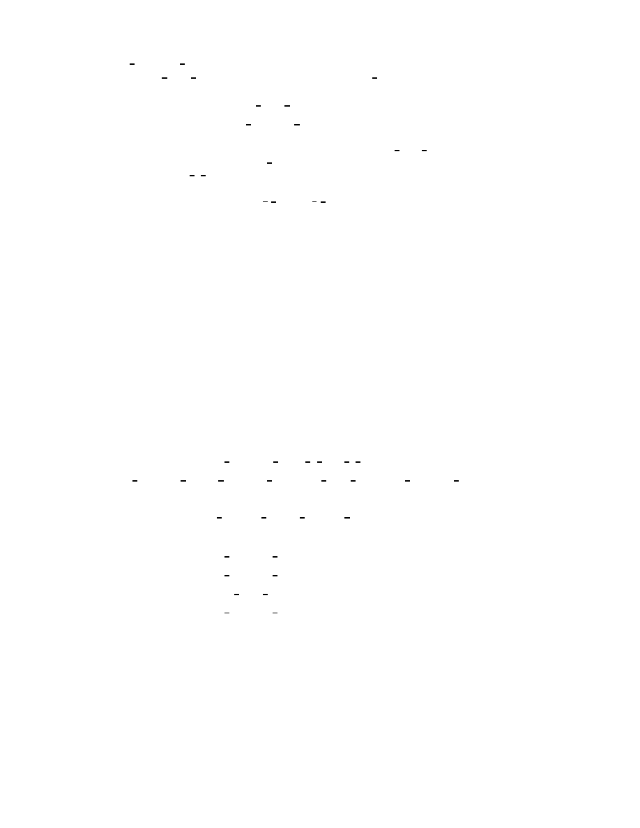
These are not a complete set of operators because ^

J

2

does not commute with ^

J

^

K

. Also

^K

3

commutes with ^J

3

but not with ^

J

2

, so it does not behave as a lowering or raising

operator, but mixes the

j

s

a

s

b

jm

i

state with all the other possible j eigenstates leaving

the eigenvalue s unchanged (Figure 2).

4.3 The Spin-

1

2

Representation

The Lorentz group has one spin-

1

2

irreducible representation,

;

1

2

0

;

0

1

2

. Translating

the Dirac spinor into the STA we nd it most convenient if it takes values in the even sub-

algebra 5, 6]. The complexication operation is identical to that of the non-relativistic

spin-

1

2

representation, multiplication on the right by i

3

.

^|

i

3

:

(121)

The basis states

mn

of this representation are,

1

2

1

2

=

1

2

(1 +

3

)

1

2

;

1

2

=

1

2

(1

;

3

)

;

1

2

1

2

= i

1

1

2

(1

;

3

)

;

1

2

;

1

2

= i

1

1

2

(1 +

3

)

(122)

16

j

s

a

s

b

j m

i

j

s

a

s

b

j m + 1

i

j

s

a

s

b

j m

;

1

i

j

s

a

s

b

j

;

1 m

i

j

s

a

s

b

j + 1 m

i

-

6

?

^K

3

^K

3

^J

+

^J

;

Figure 2: Alternative Raising and Lowering Operators for Spin-s Irreducible Representa-

tion of the Lorentz Group.

These basis states have an ideal structure, therefore they correspond most closely to the

Weyl representation.

Decomposing the

;

1

2

0

;

0

1

2

irreducible representation in terms of the SO(3) sub-

group,

(

1

2

0)

(0

1

2

)

= D(

1

2

)

D(

1

2

)

(123)

there are two D(

1

2

) doublets which are transformed into each other by the action of ^K

3

,

+

= 1

;

= i

1

^

K

3

!

+

=

3

;

=

2

:

(124)

The

doublet is identical to the D(

1

2

) representation of SO(3), the

doublet is new,

coming from the action of ^K

3

on the

doublet.

4.4 The Spin-

1

Representations

The Lorentz group has two spin-1 representations,

;

1

2

1

2

and (1 0)

(0 1). Like the

integral-spin representations of SO(3), we can construct the spin-1 representations from

the spinor representation. We use the same form,

M =

1

; ~

2

:

(125)

where ; is an arbitrary multivector to be chosen later. Since the STA and the Pauli

Algebra share the same pseudoscalar we can use the same construction as before to com-

plexify these representations,

^|M

iM:

(126)

In general, M will transform under ^V

R

as the

;

1

2

0

;

0

1

2

;

1

2

0

;

0

1

2

= 2(0 0)

2

;

1

2

1

2

(1 0)

(0 1)]

(127)

representation.

The

;

1

2

1

2

irreducible representation is obtained by choosing

; =

1

+ i

2

(128)

17

which restricts M to be vector- and trivector-valued. Inserting the

;

1

2

0

;

0

1

2

basis

states from (122) it is found that the basis states A

mn

of the

;

1

2

1

2

representation are

A

0

1

=

0

+

3

A

0

;1

=

0

;

3

A

1

0

=

1

+ i

2

A

1

;1

0

=

1

;

i

2

(129)

which is identical to the null tetrad (l n m m) of Penrose and Rindler 8, 9].

If ; is chosen to be

; =

1

+ i

2

(130)

then M will be even-valued. Further restricting (125) to the symmetric part

F =

1

2

(

1

; ~

2

+

2

; ~

1

)

(131)

then F will be bivector-valued, which corresponds to the (1 0)

(0 1) irreducible repres-

entation.

We have chosen the operation (126) to perform the complexication. Multiplication

by the pseudoscalar, i, also generates the duality operation, so by this process we only

obtain the self-dual set of basis states for F. Inserting the spin-

1

2

basis states from (122)

the basis states F

mn

are found to be

F

1

1

=

1

+ i

2

F

0

0

= i

3

F

;1

;1

=

1

;

i

2

:

(132)

Instead, if we had chosen ^|M =

;

iM to be the complexication operation, which is

consistent with choosing ; =

1

;

i

2

, we would obtain the anti-self-dual set of basis

states.

The corresponding antisymmetric part of (125)

=

1

2

(

1

; ~

2

;

2

; ~

1

)

(133)

is scalar- and pseudoscalar-valued, which is invariant under the action of ^V

R

. This cor-

responds to the scalar (0 0) irreducible representation.

Above, identifying the grades of a multivector with the representations, we have only

obtained half of the irreducible representations that should be contained in the decom-

position of the complete multivector representation (127). This is a consequence of the

minimalist route we have chosen, introducing complexication as a geometric operation.

4.5 Half-Integral-Spin Representations

We now search for half-integral-spin irreducible representations, which we expect to be

multilinear spinor-valued functions. Consider a linear spinor-valued function (a) which

transforms under ^U

R

. Its monogenic decomposition is

(a) =

M

(a) + a

(134)

where the rst term is monogenic and the second is the residual term in which dened

is by =

1

4

@

a

(a). The function (a) belongs to the

;

1

2

0

;

0

1

2

;

1

2

1

2

=

;

1

1

2

;

1

2

1

;

1

2

0

;

0

1

2

(135)

18

representation. The second term of the monogenic decomposition (134) transforms like

the

;

1

2

0

;

0

1

2

irreducible representation so the monogenic component is identied

with the

;

1

1

2

;

1

2

1

irreducible representation, a `spin-

3

2

' representation:

;

1

1

2

;

1

2

1

$

M

(a)

;

1

2

0

;

0

1

2

$

:

The monogenic functions which form the basis states for the

;

1

1

2

;

1

2

1

representation

can be constructed from the spin-

1

2

basis states and `complex'-valued linear functions

derived from the

;

1

2

1

2

representation. For example,

1

2

3

2

(a) =

1

2

1

2

0

1

(a)

(136)

is monogenic, where

0

1

(a) = a (

0

+

3

).

Now consider a bilinear spinor-valued function (a b) which transforms under ^U

R

. Its

monogenic decomposition is

(a b) =

M

(a b) + a

M

0

(b) + b

M

00

(a) + ab

1

+ ba

2

(137)

which can be further rened by taking into account the symmetry between the arguments

(a b) =

M

S

(a b) +

M

A

(a b) + a

M

0

S

(b) + b

M

0

S

(a)

+a

M

0

A

(b)

;

b

M

0

A

(a) + a b

S

+ a

^

b

A

(138)

where the subscripts S and A denote the symmetric and antisymmetric parts respectively,

M

S

(a b) =

M

S

(b a)

M

A

(a b) =

;M

A

(b a):

(139)

The function (a b) belongs to the

;

1

2

0

;

0

1

2

(

1

2

1

2

)

(

1

2

1

2

) =

;

3

2

1

;

1

3

2

;

3

2

0

;

0

3

2

2

;

1

1

2

;

1

2

1

2

;

1

2

0

;

0

1

2

(140)

representation. The are two new terms in this decomposition compared to that of a linear

spinor-valued function,

;

3

2

1

;

1

3

2

and

;

3

2

0

;

0

3

2

. Counting the degrees of freedom,

we make the following identications:

;

3

2

1

;

1

3

2

$

M

S

(a b)

;

3

2

0

;

0

3

2

$

M

A

(a b)

;

1

1

2

;

1

2

1

$

M

0

S

(a)

M

0

A

(a)

;

1

2

0

;

0

1

2

$

S

A

:

We can now proceed to nd a general half-integral-spin representation. Consider a

spinor-valued k-linear function

(a

1

::: a

k

)

(141)

19

which will transform under the action of the group as

;

1

2

0

;

0

1

2

;

1

2

1

2

:::

;

1

2

1

2

|

{z

}

k times

:

(142)

The highest-spin representation in the decomposition will be a symmetric monogenic

function which will correspond to the

;

k

+1

2

k

2

;

k

2

k

+1

2

irreducible representation. This

is conrmed by counting the degrees of freedom in this function. A symmetric spinor-

valued function in 4 dimensions has 8

(

k

+3)!

3!

k

!

real degrees of freedom. A monogenic version

of the same therefore has

8

(k + 3)!

3!k!

;

(k + 2)!

3!(k

;

1)!

= 4(k + 2)(k + 1)

(143)

real degrees of freedom which is exactly the number contained in the

;

k

+1

2

k

2

;

k

2

k

+1

2

irreducible representation.

4.6 Integral-Spin Representations

Again the integral-spin representations can be constructed from half-integral-spin repres-

entations. Consider a multivector-valued linear function constructed in the form

T(a) =

1

(a); ~

2

:

(144)

In general, T(a) will belong to the

;

1

2

0

;

0

1

2

;

1

2

1

2

;

1

2

0

;

0

1

2

(145)

representation. If

1

(a) is restricted to be monogenic, then the function will belong to

the

;

1

1

2

;

1

2

1

;

1

2

0

;

0

1

2

(146)

representation which contains the (1 1) and

;

3

2

1

2

;

1

2

3

2

irreducible representations as

the highest-spin irreducible representations. Using ; =

1

+ i

2

projects out the vector

and trivector part which corresponds to the (1 1) representation,

A(a) =

1

(a)(

1

+ i

2

) ~

2

(147)

and choosing ; =

1

+i

2

and projecting out the bivector part corresponds to the

;

3

2

1

2

;

1

2

3

2

representation,

F(a) =

h

1

(a)(

1

+ i

2

) ~

2

i

2

:

(148)

We can now generalise to to an arbitrary integral-spin representation

T(a

1

::: a

k

) =

1

(a

1

::: a

k

); ~

2

(149)

which belongs to the

;

1

2

0

;

0

1

2

;

1

2

1

2

:::

;

1

2

1

2

|

{z

}

k times

;

1

2

0

;

0

1

2

(150)

representation. If we select the monogenic, totally-symmetric part of the function, we can

restrict it to the

;

k

+1

2

k

2

;

k

2

k

+1

2

;

1

2

0

;

0

1

2

(151)

20

representation which contains the

;

k

+1

2

k

+1

2

and

;

k

+2

2

k

2

;

k

2

k

+2

2

irreducible repres-

entations as the highest-spin irreducible representations, which again correspond to the

vector-trivector and bivector parts respectively. These are both `spin-(k + 1)' representa-

tions.

We have now found the method for identifying the irreducible representations of the

Lorentz group with multilinear functions.

5 Wave Equations

So far we have restricted our attention to describing higher-weighted representations of

rotation groups with multilinear functions. The wavefunction describing a quantum-

mechanical particle depends in an arbitrary non-linear fashion on the position vector x.

The method described in this paper can be generalised to include non-linear arguments,

and thus handle these `external' spatial or spacetime degrees of freedom within the same

mathematical structure as the `internal' spin degrees of freedom.

Consider a function which transforms under ^U

R

which has linear arguments a

1

::: a

k

and non-linear arguments x

1

::: x

l

, we shall separate the linear and non-linear arguments

with a semi-colon,

(a

1

::: a

k

x

1

::: x

l

):

(152)

The non-linear arguments transform under rotation in the same manner as the linear ones,

^U

R

(a

1

::: a

k

x

1

::: x

l

)] = R( ~Ra

1

R ::: ~Ra

k

R ~Rx

1

R ::: ~Rx

l

R)

(153)

but the action of the Lie group is modied,

1

2

^L

B

(::::::)] =

1

2

B(::::::) +

P

k

i

=1

(::: a

i

B ::::::)

;

P

l

i

=1

B (x

i

^

@

x

i

)(::::::):

(154)

Each non-linear argument x

i

makes a contribution

;

B (x

i

^

@

x

i

) = (x

i

B) @

x

i

(155)

to

1

2

^L

B

. If x

i

were a linear argument then this would reduce to the same form as for

a linear argument, so this generalisation is consistent with our earlier denitions. This

operator (155) could also be interpreted as nding the component of angular momentum,

;

^|(x

^

r

), in the plane dened by B.

A similar generalisation can be made for functions which transform under ^V

R

, only the

external transformation properties of the function dier from those transforming under

^U

R

.

The Dirac equation written in the STA is

r

(x)i

3

= m(x)

0

:

(156)

This has been investigated extensively elsewhere 10, 6]. The wavefunction (x) is a spinor

function of position x. Some of the functions which form a basis for the Dirac wavefunction

can be obtained from multilinear functions by polynomial projection 1]. The l-th order

contribution can be made by setting all the arguments of a l-linear function equal to x,

l

(x) =

l

Y

i

=1

(x @

a

i

)(a

1

::: a

l

):

(157)

21

Only the symmetric part of the function will survive this procedure, the antisymmetric

parts vanish. The complete wavefunction can be expressed as a sum over all orders of

these functions.

Using the representations of the Lorentz group we found earlier, we can investigate

higher-spin wave equations. The Rarita-Schwinger equations 11] describe half-integral

spin particles. Translating these into geometric algebra, the equation describing a spin-

3

2

particle becomes

r

(ax)i

3

= m(ax)

0

(158)

with the additional condition

@

a

(ax) = 0

(159)

which ensures that the spin part of (ax) belongs to the

;

1

1

2

;

1

2

1

representation.

In general, a spinor-valued k-linear wavefunction which is symmetric in its arguments

represents a spin-(k +

1

2

) particle, it obeys

r

S

(a

1

::: a

k

x)i

3

= m

S

(a

1

::: a

k

x)

0

(160)

@

a

1

S

(a

1

::: a

k

x) = 0

(161)

where the additional condition restricts the spin part of the wavefunction to the

;

k

+1

2

k

2

;

k

2

k

+1

2

representation.

The basis functions of the k-linear wavefunction can also be obtained by polynomial

projection. The l-th order contribution to the wavefunction is obtained by setting l

arguments of a suitable (k + l)-linear function equal to x,

l

(a

1

::: a

k

x) =

l

Y

i

=1

(x @

a

(k+i)

)(a

1

::: a

k

+

l

):

(162)

The symmetry among the rst k arguments must be correct for the wavefunction that is

being described. Again, the complete wavefunction will be a sum over all orders of these

functions.

Dierent relativistic wave equations with spin corresponding to dierent represent-

ations of the Lorentz group can be explored by selecting the appropriate multilinear

wavefunctions. This presents opportunities for further investigation.

Acknowledgements

MAJA was supported by an EPSRC Research Studentship during the course of this work.

SSS is grateful to the Cambridge Livingstone Trust for funding during the course of this

work. CJLD is supported by a grant from the Lloyd's of London Tercentenary Foundation.

References

1] F. Sommen. Cliord Tensor Calculus. In

Proceedings of 22nd D. G. M. Conference,

Ixtapa, Mexico

, 1993.

2] D. Hestenes and G. Sobczyk.

Cliord Algebra to Geometric Calculus

. D. Reidel

Publishing, 1984.

3] S. F. Gull, A. N. Lasenby, and C. J. L. Doran. Imaginary Numbers are not Real|the

Geometric Algebra of Spacetime.

Found. Phys.

, 23(10):1175{1201, 1993.

22

4] C. J. L. Doran, D. Hestenes, F. Sommen, and N. Van Acker. Lie Groups as Spin

Groups.

J. Math. Phys.

, 34(8):3642{3669, 1993.

5] C. J. L. Doran, A. N. Lasenby, and S. F. Gull. States and Operators in the Spacetime

Algebra.

Found. Phys.

, 23(9):1239{1264, 1993.

6] C. J. L. Doran, A. N. Lasenby, S. F. Gull, A. D. Challinor, and S. S. Somaroo.

Spacetime Algebra and Electron Physics. In P. W. Hawkes, editor,

Advances in

Imaging and Electron Physics, Volume 95

. Academic Press, 1995.

7] S. Weinberg.

The Quantum Theory of Fields, Volume 1: Foundations

. Cambridge

University Press, 1995.

8] R. Penrose and W. Rindler.

Spinors and Spacetime, Volume 1

. Cambridge University

Press, 1984.

9] A. N. Lasenby, C. J. L. Doran, and S. F. Gull. 2-spinors, Twistors and Supersymmetry

in the Spacetime Algebra. In Z. Oziewicz, A. Borowiec, and B. Jancewicz, editors,

Spinors, Twistors, Cliord Algebras and Quantum Deformations

, pages 233{245.

Kluwer Academic, Dordrecht, 1993.

10] D. Hestenes. Observables, Operators and Complex Numbers in the Dirac Theory.

J.

Math. Phys.

, 16(3):556{572, 1975.

11] W. Rarita and J. Schwinger. On a Theory of Particles with Half-Integral Spin.

Physical Review

, 60(7):61, 1941.

23