High-Frequency Contagion of Currency Crises in Asia

*

Takatoshi Ito

a

and Yuko Hashimoto

b

June 8, 2002

Abstract

Using daily data for the period of Asian Currency Crises, this paper examines

high-frequency contagious effects among Asian six countries.

In this paper, we distinguishes “origin” (of exchange rate depreciation, or decline in

stock prices) and “affected” (currencies, or stock prices) in a sense that the origin is

defined as a currency (stock price) whose rate of depreciation over past five days is

largest and also exceeds two percent. We find evidence of high-frequency causality:

currency crisis appear to pass contagiously from “origin” to “affected”.

Then we use various trade link indices to fine that the causality of high-frequency

contagion is tied to the international trade channel. There is a positive relationship

between trade link indices and the contagion coefficient. This implies that the bilateral

trade linkage is an important means of transmitting speculative pressures across

international borders.

* The authors are grateful for comments from Munehisa Kasuya (Bank of Japan), Eiji Ogawa
(Hitotsubashi University), Shin-ichi Fukuda (University of Tokyo), and seminar participants at
2001 Summer Tokei Kenkyu-kai Conference, 2001 Fall Annual Meeting of Japanese Economic
Association, Department of Economics at Keio University, Institute of Economic Research at
Hitotsubashi University, Institute for Monetary and Economic Studies, Bank of Japan,
Department of Economics, Kyusyu University.

a

Research Center for Advanced Science and Technology, University of Tokyo. Email:

[e-mail].

b

School of Media and Governance, Keio University. E-mail:

[e-mail]

1

1. Introduction

The collapse of Thai Baht’s peg on July 2, 1997 has had devastating effects on East

Asian countries, even to panic of currency and financial crises in the region. In January

1998, when the crisis was in its most serious period, the cumulative depreciation rate

since early July 1997 was about 50 percent for most of the currencies in the region.

Among them, Indonesia Rupiah devalued by almost one sixth.

The main interpretations have emerged in the aftermath of the crises. That is, a

sudden and a huge capital outflow was one of the key sources of the initial currency

crisis. Then it caused a devaluation of currency, soar in interest rate, and clash of stock

price to launch a financial crisis. (Corsetti, Pesenti and Roubini (1998a, b), Flood and

Marion (1998), Radelet and Sachs (1998),

Yoshitomi and Ohno (1999), Ito (1997), Ito

(1999), to name a few.) Unlike the typical currency crisis that resulted mainly from the

current account and fiscal imbalances as the case of Mexico in 1994-94, the Asian crisis

was rooted mainly in financial sector fragilities. This type of

currency crisis is followed by

Russian crisis and then Brazil crisis in 1998.

In case of the Mexican Peso crash of 1994, several emerging markets fell as

investors “ran for cover” because vulnerable countries like Argentina and Brazil were

expected to be next in a series of currency crises. IMF support program in March 1995

turned out to be useful to prevent the “tequila effect”. The global financial turmoil

triggered by Russia’s default in 1998 increased risk premium in many emerging markets,

but few countries suffered currency crises attributed to Russia’s default.

1

The

contagion effect to Argentina was also avoided in case of financial crisis of Brazil in

1998-1999.

What was striking in case of Asia was (1) crises to be contemporaneous in time, and

1

Short-term interest rate soared from 59% as of June 1998 to 200% as of August 1998.

Long Term Capital Management (LTCM) suffered a heavy loss due to a sharp increase in
bond spread of developing countries and requested bail out package for the Federal
Reserve Bank. In order to avoid further default and liquidity contraction in

market, FRB cut

interest rates three times during September - November 1998.

2

(2) unprecedented rapid spread across the region. Within days after the Thai baht

floatation in early July 1997, speculators attacked Malaysia, Philippines, and Indonesia.

Hong Kong and Korea were attacked somewhat later on. The Asian Crisis differs from

other crises in its depth and width of contagion.

In this paper we examine high-frequency contagious effects among Asian six

countries (Indonesia, Korea, Malaysia, Philippines, Taiwan and Thailand) for the period

of Asian Currency Crises.

2

We use daily data in analysis to capture the day-to-day

movements in the financial market and the shift of “first victim” currency (stock price).

We attempt to answer the following questions: Given a large depreciation in the first

attacked currency, to which extent the neighboring countries suffer and how fast?

Which country is most likely to affect its depreciation to other countries during turbulent

times?

Our paper is the first in studying contagious effect that distinguishes “origin” (of

exchange rate depreciation, or decline in stock prices) and “affected” (currencies, or

stock prices) in a sense that “origin” is the first victim on one day. More specifically, we

classify daily depreciation of each country into two groups: a currency that showed the

largest depreciation among six currencies as origin and others as affected. In our

benchmark regression, we set the origin as explanatory variable. The estimated

coefficient in this regression can be interpreted as spillover from a country with the

largest depreciation to others.

We find evidence of high-frequency causality: currency

crisis appear to pass contagiously from “origin” to “affected”. In order to see whether

our classification of origin and affect reflects empirics, we check country-specific news

form Bloomberg of the date we refer to the country as origin.

The structure of the paper is as follows. In section 2, we survey previous studies on

2

Hong Kong and Singapore are precluded from the survey because (1) Hong Kong

adopted Currency board system even after the onset of crisis and therefore continued
to peg its currency to the US dollar, and (2) the depreciation of

Singaporean dollar was

relatively small.

3

currency crises and contagion

.

Section 3 summaries exchange rate and stock price of

the region during the crisis period.

In section 4 we define “origin” and “affected”. In

section 5 we present empirics and in section 6 we apply time series analysis. In section

7 we study the relationship between high-frequency contagion and trade link channel.

Section 8 concludes the paper.

2. Previous Studies on Currency Crises and Contagion

There is a growing literature on the empirical evidence on currency crises and its

contagious effects. We have seen at least three important currency crises since 1990s:

for example, Collins (1992) and Oker and Pazarbasiouglu (1997) investigate the

1992-93 crises in the European Monetary System. The Tequila crisis is surveyed in

Sachs, Tornell and Velasco (1996) and Ito (1997), among others. Corsetti, Pesenti and

Roubini (1998a, b), Radelet and Sachs (1998), Baing and Goldfajn (1999), and Berg

and Pattillo (1999) investigate the Asian crisis. What we have learned are, in general,

two main hypothesis and interpretations of the causes and the spread of crises.

According to one view, currency crisis reflects economic conditions in

countries—structural and policy distortions, and weak fundamentals. As shown in

Kaminsky, Lizondo and Reihnart (1998), some macroeconomic series behave

abnormally during periods prior to a crisis. In these cases, it may be necessary to

impose strict macroeconomic conditionality on these countries.

Another view focuses on sudden shifts in market expectations and confidence ---

caused mainly by investors’ panic and herd behavior--- regardless of macroeconomic

performance. In a financial market where participants share access to much of the

same information, a piece of new information (e.g., an small attack on a currency) can

provide a signal that lead to a revision of expectations (an information cascade) in the

4

market. The market’s perception may be interpreted by traders in other markets as an

eventual occurrence of a crisis in the near future. This effect could lead to a capital

outflow from the market and could result in an attack on currency despite of sound

macroeconomic fundamentals. In this case, countries that face difficulties in managing

reserves and capitaloutflows should be rescued with financial aid from the international

community without any conditionality.

The IMF's new precautionary facility Contingent Credit Lines (CCL), approved by the

IMF Executive Board in 1999, was designed to assist countries with strong economic

policies and sound financial systems that are seeking to resist contagion from

disturbances in global capital markets.

In addition to the crises literature, there is a lot of literature on contagion in currency

crises. There is a number of channels through which instability in financial markets

might be transmitted across countries.

One channel for contagion is the trade links. The interpretation emphasizing trade

links suggests that currency crises will

spread contagiously among countries that trade

disproportionately with one another. A currency devaluation gives a country a

temporary boost in its competitiveness, in the presence of nominal rigidities. Then its

trade competitors are at a competitive disadvantage. Deterioration in terms of trade will

also worsen competitors’ economic performance in the mid- and long- run.

Those

most-adversely-affected countries are likely to be attacked next. Glick and Rose (1998)

find the crisis spread and trade links.

Trade links may not be the only channel of crises transmission, of course.

Macroeconomic or financial similarities are not exclusive. A crisis may spread from the

initial target to another if the two countries share various economic features. Sachs,

Tornell and Velasco (1995) work on contagion in this light.

3

3

Literature based on Macroeconomic fundamentals, see Collins (1992), Flood and Marion

5

Another approach,

“Common Creditor hypothesis” approach is based on the

changes in sentiment of investors and lending agencies.

4

When financial institutions

face a default in one country, they tend to withdraw capitals not only from the country

but also from other countries so that they will avoid further default. Kaminsky and

Reinhart (2000) provide related analysis.

It should be noted that the concept of “contagion” varies from author to author.

We can think of a currency crisis as being contagious if it spreads from the initial

target, whatever reason.

5

Masson (1999a) argues based on multiple equilibria model

that crisis contagion can be referred as equilibrium switch under some economic

fundamentals conditions.

6

The alternative view is that the contagion effect is thought of as an increase in the

probability of a speculative attack on the domestic currency. See Eichengree, Rose and

Wyplosz (1996), for example.

As is well known, it is difficult to distinguish empirically between common shocks and

contagion, especially

in phase of crisis.

In both explanations above, the actual

occurrence (or an increase in likelihood of) crises depend on the existence of a (not

necessarily successful) speculative attack elsewhere in the world.

In this paper, we measure the contagion as the ratio of devaluation of currency

(decline in stock price) of one country to that of the initially targeted country. Our

definition of contagion is in line with two viewpoints above in that it is measured on the

(1994), Eichengreen, Rose and Wyplosz (1994, 1996), Otker and Pazarbasioglu (1997), to
name a few. Kaminsky, Lizondo and Reinhart (1998) is an excellent survey on empirical
literatures. Berg and Pattillo (1999) argue the crises predictability.

4

Agenor and Aizenman (1998) investigate currency crisis based on the imperfect credit

market.

5

Masson (1999 b) classifies the causes of currency crisis into three: (１) common cause

(monsoon effect), (2) fundamentals (spillover effect), and (3) trigger of first and hard hit
country (sentiment jump).

6

Flood and Marion (2000) focus currency crisis based on models of multiple equilibria.

Jeanne and Masson (2000) apply the Markov Switching model. Obstfeld (1996)

incorporates unemployment rate to the multiple equilibria model.

6

occurrence of crisis.

Our objective in this paper advances these viewpoints to analyze intra-day spillover

effect from the first attacked country, namely the high frequency contagion. We do not

take a stance on whether the initial attack is by bad fundamentals (first generation

model) or is the result of a self-fulfilling attack (second generation model). Instead, we

estimate the size of contagious effect from “ground zero”, given the incidence of the

initial attack. We then find that the high-frequency phenomenon is supportive from

trade linkage within Asia.

One of the most significant weaknesses of earlier literatures on contagion is the

absence of distinguishing “outset” from “affect” in causality relationship. In financial

market, investors are likely to respond to an attack by withdrawing capital not only from

the first attacked country, but also from neighboring countries within a few days. In this

respect, using monthly or quarterly data, even weekly data, on which many previous

analyses based, may restrict to test the existence of correlations among countries

during crisis period.

Our measure of contagion is also notable in that we can find systemically important

countries, that is, whose contagion effects are significant and sizable. In this paper we

focus on the high-frequency contagion in geographic proximity and find evidence that

the contagious channel is supported by the bilateral trade. The results are consistent

with those of Glick and Rose (1999) and Eichengreen, Wyploz and Rose (1996).

３．Exchange Rate and Stock Price during the crisis period

In the analysis of this paper we use both nominal exchange rate (against US dollar)

and stock price daily data of Indonesia, Korea, Malaysia, Philippines, Taiwan and

7

Thailand.

7

The sample period begins from January 3 1997 for exchange rate and

January 3 1994 for stock price and extends up to July 7 1999. Both the exchange rate

and stock prices data are obtained from Datastream.

Our analysis is notable in the following respects: (1) data frequency, and (2) definition

of origin. First, we use daily data in our analysis. The problem of using low frequency

data (semi-annual, quarterly, and monthly) is that it smoothes out a lot of shorter

duration interactions between the markets. Low frequency data makes it difficult to

capture every small but important event for the sample period. For instance, a large

depreciation in Thai baht had a substantial impact on Philippines peso and Indonesia

rupiah and then feed back to Thai baht. These feedback movements are, however,

diminished by the use of monthly or quarterly data. On the other hand, we should note

that it is not always appropriate to analyze with only daily data. It is often observed a

large depreciation followed by a large recovery to correct the overshooting. Detailed

data construction for regression will be shown in the following section.

Figure 1（exchange rate, June 30 1997=100）

Figure 1 shows the exchange rates of six currencies against US dollar from June 30

1997 to July 7 1999. They are normalized at 100 on June 30 1997. The behavior of

exchange rates through the crisis period varied considerably across the countries. In

Thailand, after an initial sharp depreciation (due to the floatation of baht) in July 1997,

there were a series of smaller, but still substantial depreciation over a prolonged period,

culminating in 16-17 percent depreciations at the end of August. The pressures were

eased in September in response to measures to prevent further depreciation and a

7

Stock price indices are: Jakarta Composite Index (ID), Korea South Composite Index (KR),

Composite Index (ML), Composite Index (PH), Weighted Index (TW), Bangkok Book Club (TH).

8

deterioration of economic activity. The exchange rate finally bottomed out in early 1998.

In contrast, Indonesia’s exchange rate depreciated fairly steadily starting in July

1997. Pressure on the Indonesia rupiah intensified in late September in view of

increasing strains in the financial and political sector. With the rupiah falling further

against the U.S. dollar, by early October, IMF-supported programs for Indonesia were

announced on October 31, 1997.

8

Then, Indonesia rupiah recovered temporarily in

response to the program. The limited recovery in the next few months was reversed by

large further depreciation starting in late 1997 to mid 1998.

Korea avoided substantial depreciation until October 1997, with the exchange rate

remaining broadly stable through July-October 1997. However, as Korean banks began

to face difficulties related to their short-term foreign liabilities, the exchange rate fell

precipitously during late November 1997-January 1998.

Figure 2, stock prices

Figure 2 plots stock price indices of 6 countries from January 3 1994 to July 7 1999,

with January 3, 1994=100. Stock market paints a different picture from exchange rate

market. Stock price of Thailand was at its peak in early 1990s. On the other hand, stock

prices of Indonesia, Korea, Malaysia, Taiwan continued to increase/ or had been stable

until late 1996.

Stock prices of Korea, Malaysia and Philippines began to fall in December 1996. In

Indonesia, stock prices increased through mid-1997, but fell sharply in the aftermath of

the Thai crisis. Stock prices of Taiwan also fell by some extent, but its level still exceeds

the 1994 price level. In October 1997, stock prices of Korea and Malaysia dropped

8

On November 5, 1997, the IMF’s Executive Board and Indonesia approved a three-year

Stand-By Arrangement equivalent to $10 billion. Additional financing commitments included
$8 billion form the World Bank and the Asian Development Bank, and pledges from
interested countries amounting to some $18 billion as a second line of defense.

9

significantly.

9

The declines in stock prices continued until September 1998, then

headed for recovery except Thailand and Malaysia.

4. Definitions of “origin” and “affected”

In this paper, we try to statistically analyze the size of contagion. Our basic

regression is :

Affected=const + a*Origin + e,

where Affected is a measure of change in exchange rate (stock price) of country i, and

Origin is that of first attacked country. We estimate this equation using Dynamic OLS

across countries.

We first construct an indicator that distinguishes “origin” from others that are referred

to as “affected”. To sketch our idea briefly, we first show the weekly (Friday to Friday)

origin. It is calculated based on the weekly change in exchange rate. Weekly origin is a

currency that depreciated most in a week and, on top of that, whose depreciation rate

exceeds 4%. This cut off value is arbitral.

Table1-1 plots weekly origin of exchange rate depreciation. Sample period is from July

1997 to January 1998.

Table 1-1、weekly origin

One problem using weekly change as origin is that weekly origin depends on the

choice of the day of the week. Think of a currency that depreciates 3 percent from

Thursday to Friday and then again 2 percent from Friday to Monday. Using the

definition of 4 percent depreciation starting on Friday does not pick this currency as

9

In October 1997, Hong Kong dollar was targeted of speculative attack and the Currency

Board system raised interest rate that resulted in a decline in stock prices. So, several
measures to shore up the stock market, including public funds injection, were

taken.

10

origin; while, Monday-to-Monday origin does.

Now we proceed further to determine daily origin of exchange rate (stock price). The

daily origin is derived based on weighted change of exchange rate (stock price) for

previous 5 working days. The advantage of this daily origin is that it is not sensitive to

the choice of the day of the week.

First, daily percentage change of the exchange rate is written as:

DR(t,j) = R(t, j) - R(t-1, j),

where R(t,j) is log of nominal exchange rate (country j) with respect to the US dollar at

date t. We next compute weighted average cumulative change, DRR(t,j), as follows:

DRR(t,j) = 0.5DR(t,j)+0.25DR(t-1,j)+0.125DR(t-2,j)

+0.0625DR(t-3,j)+0.0625DR(t-4,j).

The DRR is derived based on the declining weight of DRs.

10

The rationale for our measurement of origin based on DRR, not on DR is as follow; It

is often observed a large recovery of exchange rate (stock price) following a day with

large depreciation. For example, both currency A and B were heavily hit to depreciate

11 and 10 percent respectively. Next day, currency A showed a recovery of 8 percent,

while currency B did only 2 percent. It would be appropriate to interpret that currency B

was more severely targeted. DR-based-origin, however, counts A as ground zero. We

are likely to misjudge the severity of crisis should we see only the daily percentage of

10

The weights are arbitral and 0.25 for lag 1, 0.125 for lag 2, 0.0625 for lag 3 and 4. The

optimal weight (coefficient) may be computed from running VAR, but this method would not
be plausible for East Asian countries since they pegged their currencies to US dollar prior to
1997.

11

depreciation.

Our declining weight scheme is intended to avoid effect of large changes of days ago.

We do not think of a crisis as “severe” even if the rate of depreciation (decline in stock

price) is large but one-time-only. Assume even weights in calculation. A very large

depreciation 5 days ago might affect determination of the current origin. But it turns out

that the currency does not appear as origin the following day when the large one-time

depreciation days ago is excluded from the calculation. There is a possibility that a

large change in exchange rate (stock price) days ago might lead a currently non-volatile

currency as “origin” if we use even weight in calculation. Imposing declining weight

avoids this misspecification.

Our origin measure is defined analogous to our DRR as;

DOR(t,0) = “origin” = the largest DRR at each t and whose depreciation rate also

exceeds 2%.

11

Table1-2 and Table 1-3 summarize the DOR(t,0) of exchange rate and stock price,

respectively.

Table 1-2, Daily origin(exchange rate), Table 1-3 （Stock price）.

Table 1-2 lists our measure of origin of exchange rate depreciation from July 1997 to

July 1999. The table makes it straightforward to pin down the attacked date in each

country. For instance, July 1997 for Thailand, August-September for Indonesia,

October 1997- January 1998 for Korea, and after January 1998 for Indonesia. With the

economy back on the growth path after April 1999 in most of Asian countries, the

number of plots of origin declined.

Our measure of origin is consistent with journalistic

and academic references as to the beginning of the crisis period; number of different

11

The threshold of 2% is arbitral.

12

measures gives a starting date of July 1997 for Thailand, August 1997 for Indonesia,

and November 1997 for Korea.

Table 1-3 plots the origin of stock price decline. The stock in the region was at its

peak in early 1990s and then head off downward in most of countries. The rate of stock

price decline often exceeded 2 percent in early 1994.

Since late 1996, stock prices

began to fall in Thailand and fell by almost one third. The decline continued in Thailand

in early 1997. In Indonesia, stock prices increased through mid-1997, but fell

dramatically in the aftermath of the Thai crisis. The abruptly slipping exchange rates,

together with tremors in the financial and economic activities, culminated in a financial

(stock) market crisis that led to the decline in the stock prices in the region. In Korea, the

decline of stock price was temporarily interrupted in the first half of the year but

continued in the second half in the wake of banking sector crisis.

As the contagion of

exchange rate depreciation spread in the region, the downward pressure of stock prices

was further intensified in Malaysia, Korea, and Indonesia.

Since July 1998, stock price

decline originated mainly from Indonesia, Malaysia and Philippines. The rate of decline

and the frequency of large decline have been moderated since December 1998.

In wake of crisis, market sentiment is likely to be more volatile. Investors respond to

news and events that cover market fragilities and deteriorating economies of attacked

and expected-target countries. The news works as a signal to investors. In this respect,

the eruption of a signal provides investors sufficient and supportive information that an

attack would be successful; then they will concentrate their attacks on currencies (stock

price) that are expected to depreciate to very low.

Table 2 lists news release from Bloomberg. Every news release corresponds to the

timing and date of origin in Table 1-1 and Table 1-2, respectively.

Table2, exchange rate, daily origin-News

13

The table shows the news release of origin countries. For early stage of crisis, news

was relatively straightforward and was categorized to crisis-related statement; such as

authorities’ announcement on exchange rate regime, foreign reserves and IMF support

package.

In late 1997 and early 1998, news was rather related to the vulnerability of financial

and economic systems, bankruptcies and political instability. A case can be seen that

concerns on banking systems in Korea intensified the devaluation pressure at this stage.

It is also argued that exchange rate movement was highly sensitive to political instability

in Indonesia.

5．Matrices of Cumulative Contagion

In order to make our ideas of high-frequency contagion more concrete, we provide a

new indicator of contagion: contagion coefficient. This is the ratio of depreciation rate of

origin to that of affected country. This contagion coefficient measures high-frequently

spreading of financial crisis (depreciation, or decline in stock

prices) from origin (first

attacked country) across other affected countries.

The contagion coefficient is calculated as:

CC(t,i)= DRR(t,i)／ DOR(t,0)，

where i≠0. Table 3-1 reports CC(t,i) for exchange rate and Table 3-2 to Table 3-4

report CC(t,i) for stock price. Sample period starts July 1 1997 and ends July 7 1999.

12

12

The sample period includes when Malaysia began to peg its currency to US dollar starting

at September 1, 1998. The daily percentage change in exchange rate is close to zero and
so is the DRR in Malaysia after September 1998. Therefore, Malaysia is virtually excluded
from “origin” for this period. Thus, we do not need to explicitly impose structural change on
Malaysia when we run regressions in the following section.

14

Negative sign of CC indicates the opposite movements of exchange rate (stock price)

between origin and affected countries. In the case of exchange rate, devaluation of

origin country leads to appreciation of affected countries. On the other hand, positive

sign of CC indicates that the direction of exchange rate (stock price) movements

between Origin country and affected countries are the same. That is, devaluation of

origin country leads to a devaluation of affected countries: contagion.

Table3-1 plot of CC (exchange rate), 3-2〜3-5 (stock price)

Table 3-1 shows CC(t,i) for exchange rate. As shown in Table 1-2, frequency of

origin drastically decreases since June 1998. Exchange rates had been back on

recovery track by the summer 1998. Most of crisis (large depreciation) after July 1998

were from Indonesia. Therefore, we divide sub-sample period into two in the case of

Indonesia.

13

Specifically, for origin of Indonesia, we calculate CC(t,i) for two

sub-sample periods, crisis period (1997/7/1-1998/6/17) and recovery period

(1998/6/18-1999/7/7), in addition to whole sample period (1997/7/1-1999/7/7).

In the case of exchange rate, there are 87 instances that are regarded as origin in

terms of our definition. Out of them, 61 instances are of Indonesia, 14 instances of

Korea and 6 instances of Thailand.

Stat (statistics) in Table 3-1-Table 3-4 tests the null of zero.

14

The null measures

insignificant difference of the rate of depreciation (decline) between origin and affect

countries: that is, there exists no significant high-frequency contagion from origin to

affected.

13

After June 1998, most of currencies in East Asia went back on the recovery track, while

Indonesia rupiah was trending down. So, the sign of CCs on Indonesia at this period is likely
to be negative.

14

Calculation is as follows: Stat = (x^-x0)/(square root of variance / square root of NOB),

where x^:average; x0:(Null)=0 and x0 is the ratio of DOR/DRR (CC).

15

The significance of estimated coefficients varies according to sample periods and

countries. The coefficients of contagion originating from Thailand and from Philippines

are, in many cases, negative. Shortly after the onset of currency crisis when Thai baht

and Philippines peso, two first-hard-hit currencies, devalued, other currencies were not

severely hit and remained their value to US dollar. The contagion coefficients of them

are, however, not significantly different from zero.

The sign of coefficients of affected countries, a case for either Indonesia or Korea is

origin, are positive and significantly different from zero: depreciation of Indonesia and of

Korea induces high-frequency contagion effect. That is, we find evidence of significant

high-frequency contagion originating from Indonesia to Malaysia, Indonesia to Thailand,

Korea to Malaysia, Korea to Thailand and Korea to Indonesia.

The contagion coefficients originating from Indonesia are positive and significant in all

but Korea over the sample period up to June 17, 1998. After June 17, 1998, the results

reverse: the contagion coefficient is significantly positive only in Korea and

insignificantly different from zero or significantly negative in other countries.

In sum, depreciation of Indonesia and of Korea has significant high-frequency

contagion effect on other currencies but not vice versa.

Table 3-2 - Table 3-4 presents CC(t,i) of stock prices. Table3-2 shows CC for whole

sample period; Table3-3 and Table3-4 report pre-crisis and post crisis period,

respectively.

For Indonesia, there are 2 instances to be origin for pre-crisis period and 28

instances for post-crisis period. For Korea, 3 instances for pre-crisis and 44 for

post-crisis; for Malaysia, 4 for pre-crisis and 25 for post-crisis. In these 3 countries,

number of instances regarded as origin dramatically increased after the onset of crisis.

On the other hand, for Philippines and for Thailand, the instances do not make a big

change. For Philippines, there are 12 instances for pre-crisis period and 15 instances

16

for post- crisis period. For Thailand, 17 for pre-crisis and 16 for post-crisis. For Taiwan,

in contrast to other countries, the instances surprisingly decreased from 16 for pre-crisis

period to 6 for post-crisis period. The instances as origin as a whole dramatically

increase for post-crisis.

Contagion coefficients of ASEAN countries for the post-crisis period turn to be

significantly positive, or the magnitude of contagion coefficients become larger. A case

for Korea to be origin,, contagion coefficients for pre-crisis period are negative, while

they become positive and significantly different from zero for post-crisis period.

In sum, we may conclude that high frequency contagion of stock prices has been

intensified through currency crises period.

6．Regression

In the previous section we find high-frequency contagion in both exchange rates and

stock prices among Asian countries. We also note that the stock price high-frequency

contagion becomes intensified after the crisis.

In this section, we present some formal econometric results to statistically show to

what extent the depreciation of exchange rate (decline of stock prices) of first attacked

country, namely origin, affects others.

The regressions are estimated using Dynamic OLS (DOLS) method in the following

specification:

affected(t,i) = const + a1*origin(t, 0)

+b1*dorigin(t+1, 0) + b2*dorigin(t, 0) +b3*dorigin(t-1, 0) + e,

where i≠0. Here, affect(t,i) is DRR, origin(t,0) is DOR defined in section 4 above, and

dorigin(t,0) = DOR(t,0)-DOR(t-1,0). DOLS method provides efficient estimator if the

17

regressor is cointegrated or endogenous. By including the current change as well as

the past and future changes of regressor in the regression, we are able to maintain the

strict exogeneity of the regressor, the origin (DOR). The order of leads and lags of

changes of regressor is arbitral; we set 1 in the analysis below. Standard error for point

estimate of a1 is recalculated based on the DOLS residuals and then adjusted to the

sample period of recalculated augmented cointegrating regression.

15

For purposes of comparison, 2 types of estimation are done: (1) the regressor,

origin(t,j), includes every “origin”. That is, we do not distinguish the first attacked

“country”. We call this regressor “pooled origin”. And, (2) country specific origin(t,j).

That is, we run regression on origin according to country. We call this “country-specific

origin”.

The expected sign of point estimate of a1 is positive if there exists high-frequency

contagion. Estimation results are summarized in Table 4-1 and Table 5-1〜 Table 5-8.

Table4-1 exchange rate, DOLS

Table 4-1 shows the estimates for exchange rate. Sample period covers from July 1

1997 to July 7 1999. The dependent variables are “affected” countries and independent

is “origin”.

The first row of the table shows the regression results on pooled origin. The

second and the third rows of the table show the estimation results with country-specific

origin of Indonesia and Korea, respectively.

16

Estimation results show that estimated coefficients in Korea, Malaysia, Philippines

and Thailand on pooled origin are positive and significantly different from zero. The sign

of estimated coefficient is, however, negative in Indonesia. The result for Indonesia can

be interpreted as that the behavior of Indonesian rupiah is slightly different from others.

15

See Hayashi (2000) for details.

16

DOLS regressions include leads and lags in both OLS and residual regressions and

therefore, reduce degree of freedom. Thus, Thai origin is precluded from the regression.

18

For example, most of the currencies in East Asia are back on recovery track around

April 1998, while Indonesia rupiah has been trending down.

Estimated coefficients in

Korea, Malaysia and Philippines are significantly different

from zero and range from 0.12 to 0.19. In contrast, estimated coefficient is not

significant in Taiwan; that is, the high-frequency contagion is not significantly seen in

Taiwan. This finding is consistent with the fact that Taiwan is one of the least hit and the

least contagious suffered countries in 1997.

Now we see estimation results on country-specific origin. A case for Indonesia as

origin, contagion coefficients in Philippines and Taiwan are significant. Contagion

coefficients in Malaysian and Thailand are small but significantly different from zero. In

contrast, contagion coefficient in Korea is significantly negative. Indoneisa rupiah

severely depreciated following the Korea won in early 1998. The movement of Korean

won might be opposite to that of Indonesia: when Indonesia was hard hit, Korean won

was on the recovery track. Therefore, the coefficient of Korea on rupiah is likely to be

negative.

There seems a significant high frequency contagion in Indonesia and Malaysia in

case of Korea origin. The estimated coefficient in Indonesia is 0.68 and significantly

different from zero. The estimated coefficient in Philippines is 0.24 but is not

insignificant. The estimated coefficient in Thailand, however, is significantly negative.

We find two important messages from Table 4-1. First, there exists high-frequency

contagion among East Asian countries. Our contagion coefficients of affected countries

are positive and statistically significant in most countries. Second, estimation results on

country-specific origin show that contagion effects from Indonesia and from Korea are

significant in some countries.

17

17

Baig and Goldfajin (1999), for instance, use VAR to analyze impulse response among

Indonesia, Korea, Malaysia, Philippines and Thailand and conclude that the impulse shock
of Indonesia has significant effect on other countries. Our findings are consistent with these
results.

19

Table5-1〜Table5-7 Stock Price DOLS

Table 5-1-Table 5-7 presents the estimate results for stock prices. We run

regressions for three sample periods: whole sample period (January 1994-July 1999),

pre-crisis (January 1994-June 1997), and post-crisis period (July 1997-July 1999).

Due to the degree of freedom, regressions for pre-crisis period for either Indonesia,

Korea or Malaysia to be origin are excluded. The regression estimates on origin in the

case of Taiwan is not shown for post-crisis period.

Estimates results of contagion coefficients on pooled origin are shown in Table

5-1. Contagion effects are significant in all countries for the whole sample period. The

estimated coefficient is significantly negative in Korea for both pre- and post- crisis

periods. However, the magnitude of coefficient becomes smaller for post crisis period.

The magnitude of estimated coefficient in Taiwan, on the other hand, declined

sharply after the crisis. Taiwan was less influenced from high-frequency contagion.

Table 5-2 to 5-7 presents estimates results on country-specific origin.

Table5-2 shows the estimates results on Indonesia origin. The estimated coefficients

are significantly positive in both Malaysia and Philippines.

Table5-3 is the case of Korea as origin. All estimated coefficients, except Thailand,

are significantly negative. The magnitude of estimated coefficients for post-crisis period

becomes larger (in negative) in Indonesia and Malaysia. These are consistent with the

fact that Korean stock price index declined sharply in late 1997 while stock prices in

other countries remained stable.

Table5-4 reports results on Malaysia origin. Estimated coefficient is significantly

positive only in Thailand. Most of the estimates are significantly negative.

The results of Philippines origin are summarized in Table 5-5. The estimated

coefficients in Indonesia, Korea and Malaysia are significantly positive for both pre- and

post- crisis periods. Sign of coefficient turns to be positive (but insignificant) in Thailand

20

for post-crisis period.

Table5-6 presents the results of Taiwan origin. The coefficients are significantly

estimated.

The estimates results of Thailand origin are shown in Table 5-7. The sign of coefficient

turns to be positive (insignificant) in Indonesia after the crisis. In contrast, they turn to be

negative in Taiwan (significant) and in Malaysia (insignificant).

In sum, the regressions on pooled origin and on country-specific origin do not report

significant difference. The sign and significance of estimated coefficients vary from

country to country depending on origin by individual countries. The estimates results on

pooled origin, however, clearly show the existence of high-frequency contagion in the

stock market, especially after the crisis. This finding strongly reflects the change of

exchange rate regime in Asian countries, among various factors in the markets.

18

7．Contagion and Trade Link Channel

In this section we provide empirical support for high-frequency contagion channel.

Why crises spread and why they tend to be regional are explained at least three ways:

macroeconomic similarities, financial market integration and trade linkage.

In financial

market, investors pull their capital out of countries in the same region of the first-hit

country soon after the country is targeted as a speculative attack. Their choice of

countries relies on macroeconomic and financial fundamentals to some extent. From

the perspective of most empirical speculative and crisis models, however, it is hard to

understand why crises tend to spread be regional, at least at an early stage of crisis. As

shown in Glick and Rose (1999), performances of macroeconomic fundamentals are

not necessarily similar among crises countries.

18

Malliaropulos (1998) , for example, reports negative relationship between the return of

stock prices and the change in exchange rates.

21

One of the reasons why investors withdraw capital not only from the first targeted

country but also from neighboring countries lies in the regional trade linkage.

Devaluation of the first-hit country results in price advantage in the short run. Then,

countries lose competitiveness when their trading partners devalue. They are therefore

more likely to be attacked in prospect of their worsened trade balance associated with

its trade competitors’ devaluation that might create expectation of deterioration of the

economy in the future. In practice, it takes some time until current trade balance

deterioration will be reflected in GDP and other economic data. In theory, however,

investors predict the future devaluation at the onset of speculative attack based on the

trade linkage mechanism. Investors are likely to sell currencies of trading partners in

anticipation of a fall and induce devaluation pressure in the market at the time. This is

the trade link channel that devaluation of the first-hit currency contemporaneously spills

over to regional countries.

For many Asian countries, a large portion of their goods is directed to the United

States, Japan, EU, and Intra Asia.

19

It is tempting to believe that some direct and

indirect trade linkages due to bilateral and third-market competition were instrumental in

repeated rounds of competitive devaluation. There are a large volume of studies on

contagion and trade link (Eichengreen and Rose (1999), Glick and Rose (1999), Forbes

(2000), Kaminsky and Reinhart (2000) to name a few), and they support the evidence of

relationship between the contagion and trade links.

In the following we check evidence of the contagion and trade link channel using

three measures.

19

Export share within Asia varies between countries, but it ranges from 25% to 45%.

22

7．１ Compete Effect

There are at least three different types of explanations for why contagion spreads in

geographic proximity, especially by international trade. The first relies on competitive

effect analyzed by Gerlach and Smets (1995), Corsetti, Pesenti, Roubini and Tille

(2000). Devaluation of hard hit country raises the relative export price of its trading

partners and competitors. Then, market participants may expect declining trade

balance due to weakened price competitiveness and are likely to withdraw capital out of

these countries. We provide two indices, export share and Direct Trade Linkage Index

(DTLI), for analysis.

Table６

Table 6 presents the export share in intra-Asia trade for each of 5 countries

(Indonesia, Korea, Malaysia, Philippines and Thailand) for 1996-1999.

20

The export

share of country m is the ratio of export from country m to country n divided by the total

export of country m.

Next, we define Direct Trade Linkage Index（DTLI） as

21

DTLI

0i

= 1- (x

i0

- x

0i

) / (x

i0

+ x

0i

).

Here, x

mn

denotes bilateral exports from country m to n. Subscript o and i indicate

home country and its direction of trade, respectively. The index DTLI

0i

is higher than 1

if exports from country o to country i is greater than imports of o from i. The index lies

between 0 and 1 if imports exceed exports. The index is close to 1 if the bilateral trade

between countries o and i are almost equal.

20

IMF、Direction of Trade, CD-Rom (2000).

21

See Glick and Rose (1999).

23

For example, when the bilateral trade balance between countries o and i are positive,

then devaluation of country o accelerates the export of country o and, in contrast,

depresses the export of country i to country o. Thus, contagion coefficient (CC) is

expected to be positively related to DTLI

0i

for DTLI

0i

>1. On the other hand, for DTLI

0i

<1, CC may be small and/or negative.

Table ７

Table 7 summarizes DTLI

0i

.

Figure 3、 Figure 4

Figure 3 plots the contagion coefficients (CC) and the export share, and figure 4 plots

the CCs and DTLI

0i

. The CCs are measured on the vertical axis in both figures. The

export share and DTLI are measured on the horizontal axis in figure 3 and figure 4,

respectively.

In each figure, there exists positive relationship between CCs and export share, and

between CCs and DTLI. The correlation coefficient of each figure is 0.329 and 0.258,

respectively.

7．２ Income Effect

The second measures to relate trade links to spread of crisis is income effect. (See for

example, Forbes(2000).) Imports of crisis country declines due to the downturn of

economic activities and therefore the income level decreases. Then, its trading partners

also suffer negative macroeconomic effects because of reduction in exports to hard hit

country. Countries with large export share to first hit country suffer negative income

24

effect of the crisis country and, therefore, they are also likely to be attacked.

Table8 Figure 5

Table8 reports the income effect index. The index is represented by the export (from

“affected” to “origin”) to GDP ratio. Figure 5 plots the index on the horizontal axis and

Contagion Coefficient on the vertical axis. There is a positive relationship between the

income effect and the contagion. This correlation coefficient is 0.357. This result implies

that countries with large export share to origin country are likely to suffer currency crisis.

7．３ Cheap Import Effect (bilateral trade effect, supply effect)

The third measure of trade channel is the Cheap Import Effect (also called either

bilateral trade effect or supply effect). Devaluation of hard hit currency drives export

price down, which is equivalent to the decline in import price in its trading partners. With

nominal income and other conditions held constant, a decline in import price raises

disposable income and, therefore, improves welfare of the countries. It is also expected

that the terms of trade in affected countries improve because the import price from

origin country decreases while the export price of these countries held constant.

In this case, in contrast to other two explanations above, devaluation of hard hit

country may affect positive effect to its trading partners. As shown in Corsetti, Pesenti,

Roubini and Tille (2000) and Forbes (2000), speculative pressures may not be

transmitted to trading partners through this channel if the import price effect in affected

countries dominates.

Table9 Figure 6

25

Table 9 presents the Cheap Import Effect. The index is calculated as the import from

origin country divided by GDP. The larger the index, the larger the import from the

origin country. The contagion coefficient (CC) and the index are expected to be

negatively correlated because the large devaluation in origin country may improve its

trading partners’ welfare in terms of the decline of import price, and therefore trading

partners are less likely to suffer crisis.

Figure 6 plots the CC and the index. It is obvious from the figure that the index has

positively related to CC. The correlation coefficient is 0.384. This result means that the

cheap import effect does not work asto improve welfare of affected countries. Rather,

the negative effect of devaluation in origin country, especially the effect from weakened

price competition, has been dominant across international trade.

correration coefficient
export share

0.329

DTLI

0.258

income

0.357

cheap import

0.384

All of the tests above are consistent. Various measures support our high-frequency

contagion and trade link channel.

8．Concluding remarks

Using daily data for the period of Asian Currency Crises, this paper examines

high-frequency contagion among Asian six countries.

We find evidence of high-frequency contagion among Asian countries in both

exchange rate and stock prices markets. We also find the significant contagious effects

originating from Indonesia and Korea.

Surprisingly, our high-frequency contagion is tied to the international trade channel.

26

There is a positive relationship between trade link indices and our contagion index. This

implies that the bilateral trade linkage is an important means of transmitting speculative

pressures across international borders.

References

Agenor, Pierre-Richard and Joshua Aizenman, 1998, Contagion and Volatility with

Imperfect Credit Markets, IMF Staff Papers Vol. 45, No.2, 207-235.

Baig, Taimur and Ilan Goldfajn, 1999, Financila Market Contagion in the Asian Crisis,

IMF Staff Papers Vol. 46, No.2, 167-195.

Berg, Andrew and Catherine Pattillo, 1999, Are Currency Crises Predictable? A test,

IMF Staff Papers Vol.46, No.2, 107-138.

Collins, Susan, 1992, The Expected timing of EMS realignments: 1979-83, NBER

Working Paper No. 4068.

Corsetti, Giancarlo, Paolo Pesenti, and Nouriel Roubini, 1998a, What Caused the Asian

Currency and Financial Crisis? Part I: A Macroeconomic Overview, NBER Working

Paper No. 6833.

Corsetti, Giancarlo, Paolo Pesenti, and Nouriel Roubini, 1998b, What Caused the Asian

Currency and Financial Crisis? Part II: The Policy Debate, NBER Working Paper No.

6834.

27

Corsetti Giancarlo, Paolo Pesenti, Nouriel Roubini and Gerdric Tille, 2000, Competitive

Devaluations: Toward a Welfare-Based Approach, Journal ofInternational Economics

51, 217-241.

Eichengreen, Barry, Andrew Rose and Charles Wyplosz, 1994, Speculative Attacks on

pegged exchange rates: an empirical exploration with special reference to the

European monetary system, NBER Working Paper No. 4898.

Eichengreen, Barry, Andrew Rose and Charles Wyplosz, 1996, Contagious Currency

Crises: First Tests, Scandinavian Journal of Economics 98(4), 463-484.

Flood, Robert and Nancy Marion, 1994, The size and timing of devaluations in

capital-controlled developing economies, NBER Working Paper No. 4957.

Flood, Robert and Nancy Marion, 1998, Perspectives on the Recent Currency Crisis

literature, NBER Working Paper No. 6738.

Flood, Robert and Nancy Marion, 2000, Self-Fulfilling risk predictions: an application to

speculative attacks, Journal of International Economics 50, 245-268.

Forbes, Kristin, 2000, The Asian Flu and Russian Virus: Firm-Level Evidence on How

Crises are Transmitted Internationally, NBER Working Paper No. 7807.

Gerlach, Stefan and Frank Smets, 1995, “Contagious Speculative Attacks”, European

Journal of Political Economy 11, 45-63.

28

Glick, Reuven and Andrew Rose, 1999, “Contagion and trade Why are currency crises

regional?”, Journal of International Money and Finance 18, 603-617.

Ito, Takatoshi, 1997, Capital flow and Emergin market, Lessons from Mxico crisis

(Sihon ido to sinkou sijou- Mexico crisis no kyoukun), Keizai kenkyu 48(4), 289-305, in

Japanese.

Ito, Takatoshi, 1999, Capital Flows in Asia, NBER Working Paper, No. 7134.

Kaminsky, Graciela, Saul Lizondo and Carmen M. Reinhart, 1998, Leading Indicators of

Currency Crises, IMF Staff Papers Vol.45, No.1, 1-48.

Kaminsky, Graciela, and Carmen M. Reinhart, 2000, On crises, contagion, and

confusion, Journal of International Economics Vol. 51, No. 1, 145-168.

Malliaropulos, Dimitrios, 1998, International stock return differentials and real exchange

rate changes, Journal of International Money and Finance 17, 493-511.

Masson, Paul, 1999 a, Contagion: macroeconomic models with multiple equilibria,

Journal of International Money and Finance 18, 587-602.

Masson, Paul, 1999 b, Contagion: monsoonal effects, spillovers and jumps between

multiple equilibria, in Agenor, P.R., M. Miller, D.Vines and A. Weber (eds.), The Asian

Financial Crisis: Causes, Contagion and Consequences, Cambridge University Press.

Obstfeld, Maurice, 1996, Models of Currency crises with self-fulfilling features,

European Economic Review 40, 1037-1047.

29

Otker, Inci and Ceyla Pazarbasioglu, 1997, Speculative attacks and macroeconomic

fundamentals: evidence from some European Currencies, European Economic Review

4, 847-860.

Radelet, Steven, and Jeffrey Sachs, 1998, The Onset of the East Asian Financial Crisis,

NBER Working Paper No. 6680.

Sachs, Jefrrey, Aaron Tornell and Andres Velasco, 1996, Financial Crises in Emerging

Markets: The Lessons from 1995, NBER Working Paper, No. 5576.

Yoshitomi, Masaru and Kenichi Ohno, 1999, Capital-Account Crisis and Credit

Contraction: The New Nature of Crisis Requires New Policy Responses, ADBI Working

Paper No.2.

 
 

30

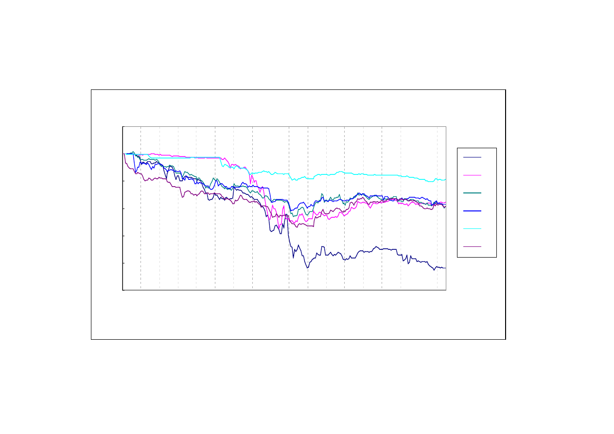
Figure 1: Asia Exchange Rates

June 30, 1997 = 100

0

20

40

60

80

100

120

30

6

1997

21

7

1997

11

8

1997

1
9

1997

22

9

1997

13
10

1997

3

11

1997

24
11

1997

15
12

1997

5
1

1998

26

1

1998

16

2

1998

9
3

1998

30

3

1998

20

4

1998

11

5

1998

1
6

1998

22

6

1998

ID

KR

MY

PH

TW

TH

31

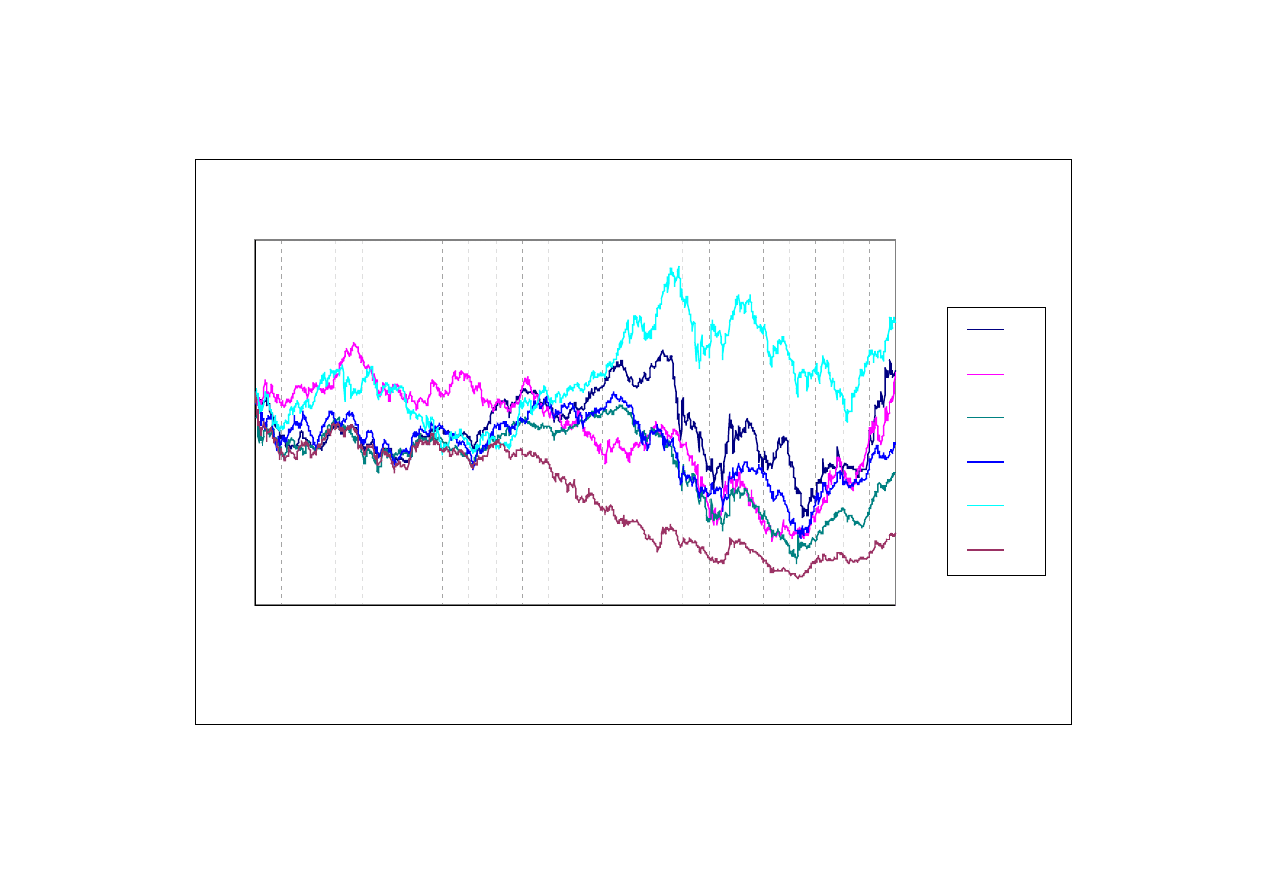
Figure 2: Asia Stock Price Index

 January 3, 1994 = 100

0

20

40

60

80

100

120

140

160

180

4 1

 19

94

29

 3 

19

94

21

 6 

19

94

13

 9 

19

94

6 1

2 1

99

4

28

 2 

19

95

23

 5 

19

95

15

 8 

19

95

7 1

1 1

99

5

30

 1 

19

96

23

 4 

19

96

16

 7 

19

96

8 1

0 1

99

6

31

 12

 19

96

25

 3 

19

97

17

 6 

19

97

9 9

 19

97

2 1

2 1

99

7

24

 2 

19

98

19

 5 

19

98

11

 8 

19

98

3 1

1 1

99

8

26

 1 

19

99

20

 4 

19

99

ID

KR

MY

PH

TW

TH

32

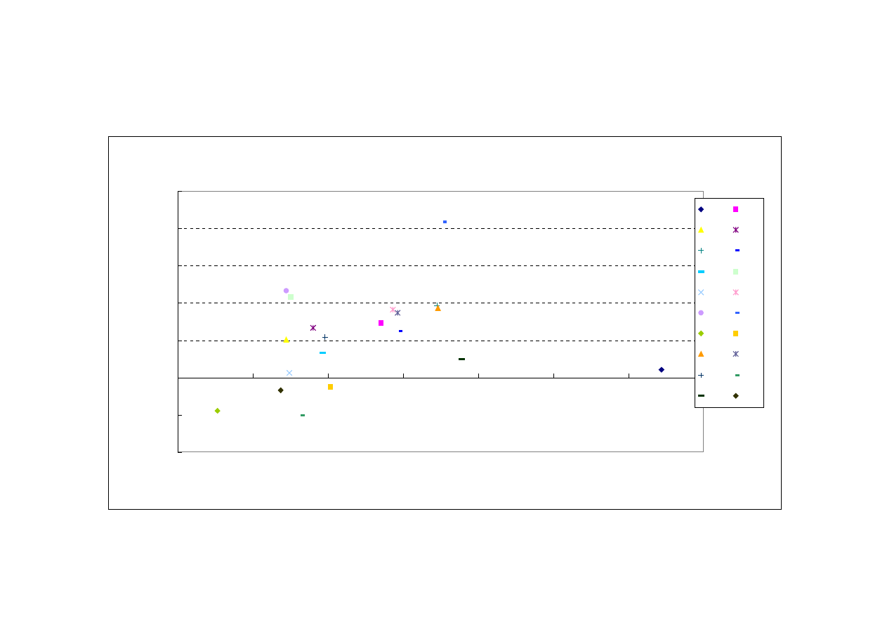
Figure 3

Export share and Contagion coefficient

-0.2

-0.1

0

0.1

0.2

0.3

0.4

0.5

0

1

2

3

4

5

6

7

export share

contagion coefficient

idkr

idmy

idph

idth

krid

krmy

krph

krth

myid

mykr

myph

myth

phid

phkr

phmy

phth

thid

thkr

thmy

thph

33

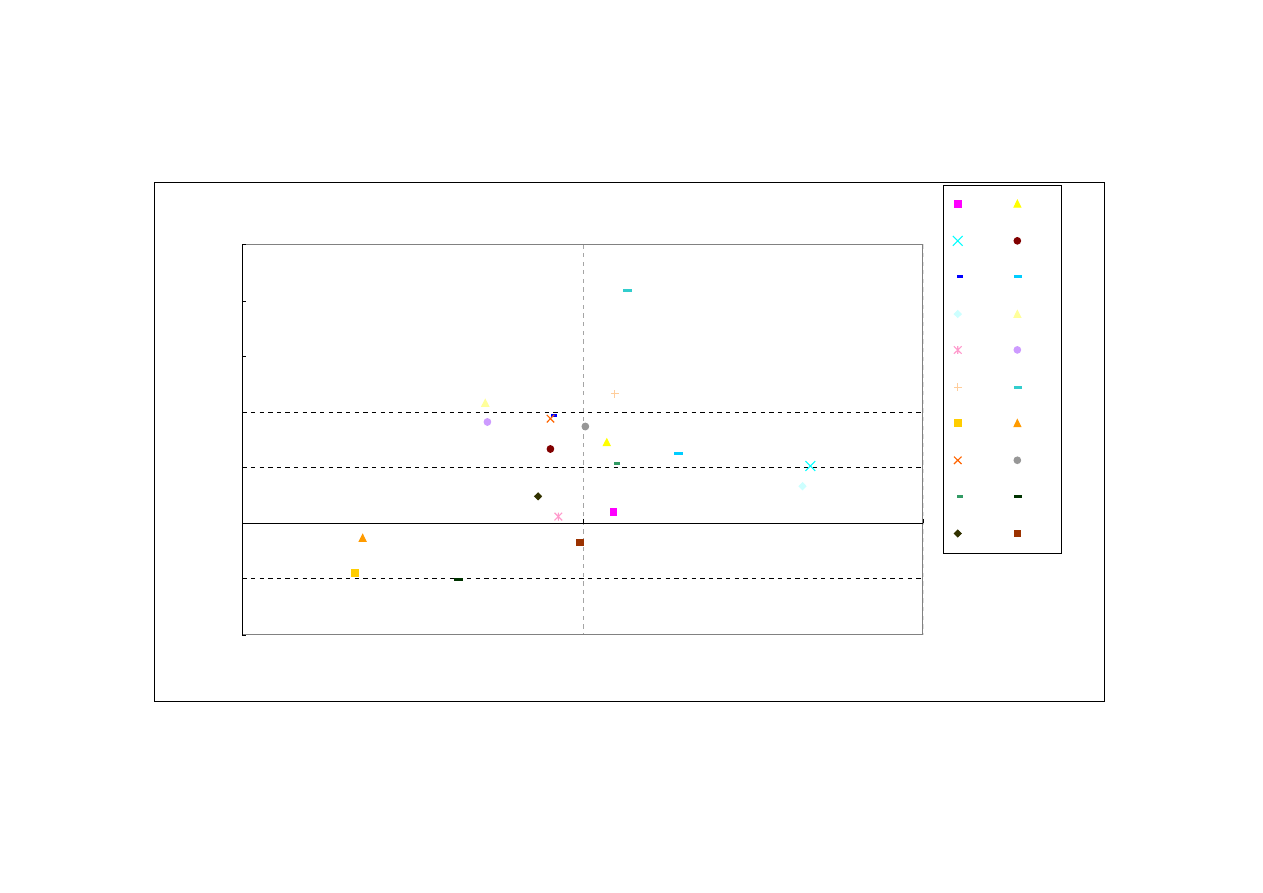
Figure 4

Trade linkage and Contagion

-0.2

-0.1

0

0.1

0.2

0.3

0.4

0.5

0.000

1.000

2.000

Direct trade linkage index

C

o

nta

gi

o

n co

ef

fi

ci

ent

idkr

idmy

idph

idth

krid

krmy

krph

krth

myid

mykr

myph

myth

phid

phkr

phmy

phth

thid

thkr

thmy

thph

34

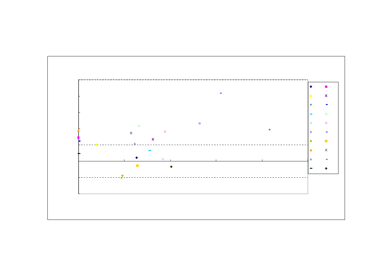
Figure 5

Income effect and Contagion coefficient

-0.2

-0.1

0

0.1

0.2

0.3

0.4

0.5

0

0.05

0.1

0.15

0.2

0.25

imcome effect

contagion coefficient

idkr

idmy

idph

idth

krid

krmy

krph

krth

myid

mykr

myph

myth

phid

phkr

phmy

phth

thid

thkr

thmy

thph

35

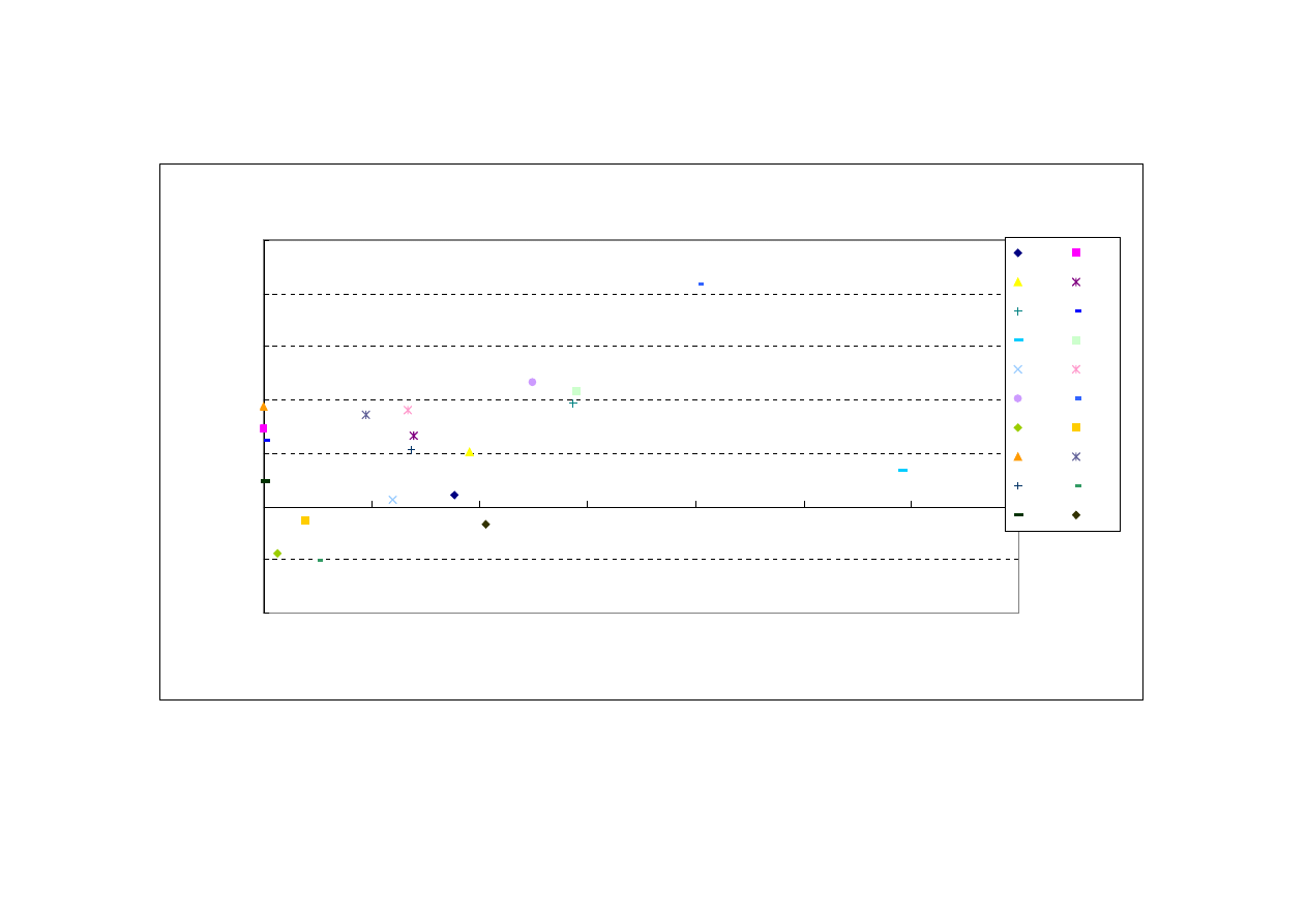
Figure 6

Cheap import effect and Contagion coefficient

-0.2

-0.1

0

0.1

0.2

0.3

0.4

0.5

0

0.05

0.1

0.15

0.2

0.25

0.3

0.35

cheap import effect

contagion coefficient

idkr

idmy

idph

idth

krid

krmy

krph

krth

myid

mykr

myph

myth

phid

phkr

phmy

phth

thid

thkr

thmy

thph

36

Table 1-1

Weekly Origin  (weekly change,

Friday close to Friday close)
July 1997-January 1998

Week

devaluation 

1997-98

Origin

rate(%)

Jul-1

TH

-10.11

Jul-2

PH

-7.95

Jul-3
Jul-4

TH

-5.75

Aug-1
Aug-2
Aug-3

ID

-10.13

Aug-4

TH

-4.52

Aug-5

ID

-7.51

Sep-1

TH

-9.40

Sep-2
Sep-3

PH

-4.81

Sep-4

Oct-1

ID

-13.84

Oct-2
Oct-3
Oct-4
Oct-5

TH

-5.99

Nov-1

6.44

Nov-2

TH

-4.94

Nov-3

KR

-4.85

Nov-4

KR

-8.13

Dec-1

ID

-7.76

Dec-2

ID

-32.93

Dec-3
Dec-4

Jan-1

KR

-17.63

Jan-2

ID

-18.32

Jan-3
Jan-4

ID

-57.18

Jan-5

Notes

: Authors' calculation.

Data source: Datastream

37

Table 1-2

Daily Origin

(cumulative weighted daily change)

July 1997-January 1998

devaluation

Origin

rate(%)

1997

7

2

TH

-3.40364

1997

7

3

TH

-2.21693

1997

7

4

TH

-2.05508

1997

7

14

PH

-5.2999

1997

7

21

ID

-2.82547

1997

7

23

TH

-2.06453

1997

8

15

ID

-2.9887

1997

8

18

ID

-3.23057

1997

8

27

ID

-2.92794

1997

8

28

ID

-3.19417

1997

9

2

ID

-2.39097

1997

9

3

TH

-2.80691

1997

9

4

TH

-3.74387

1997

9

18

PH

-2.06418

1997

9

29

ID

-2.38314

1997

9

30

ID

-2.32572

1997

10

1

ID

-3.19195

1997

10

3

ID

-4.31997

1997

10

6

ID

-2.56053

1997

10

20

TW

-2.45012

1997

11

20

KR

-5.51712

1997

11

25

KR

-2.24082

1997

11

28

KR

-2.92259

1997

12

1

KR

-2.2079

1997

12

2

KR

-2.8175

1997

12

3

TH

-3.65745

1997

12

8

KR

-5.38599

1997

12

9

KR

-6.87652

1997

12

10

KR

-6.73185

1997

12

11

KR

-8.01844

1997

12

12

ID

-10.97388

1997

12

15

ID

-6.71699

1997

12

16

TH

-3.65745

1997

12

22

KR

-10.11797

1997

12

23

KR

-10.11797

1997

12

24

ID

-4.32178

1997

12

25

ID

-2.33994

1997

12

31

KR

-3.96039

Notes

: Authors' calculation.

Data source: Datastream

38

T able   1 - 2 (c o n t in u e d)

D aily O r ig in

(c u m u lat iv e  w e ig h t e d da ily  c h a n g e )

F e br u ar y  1 9 9 8 - J u n e   1 9 9 8

de va lu at io n

O r ig in

r a t e (% )

1 9 9 8

1

2

ID

- 1 4 .3 7 7 4 7

1 9 9 8

1

5

ID

- 1 3 .0 8 0 5 1

1 9 9 8

1

6

ID

- 1 1 .9 3 4 8 9

1 9 9 8

1

7

ID

- 7 .5 7 2 1 6

1 9 9 8

1

8

ID

- 1 8 .3 0 8 7 1

1 9 9 8

1

1 2

T H

- 2 .3 8 7 4 5

1 9 9 8

1

1 6

ID

- 4 .0 0 9 5 5

1 9 9 8

1

1 9

ID

- 7 .8 7 1 3 2

1 9 9 8

1

2 0

ID

- 4 .7 1 6 5 6

1 9 9 8

1

2 1

ID

- 1 1 .0 9 8 4 4

1 9 9 8

1

2 2

ID

- 1 2 .8 6 5 7 7

1 9 9 8

1

2 3

ID

- 1 2 .7 7 3 9 8

1 9 9 8

1

2 6

ID

- 3 .8 4 5 5 2

1 9 9 8

2

1 2

M Y

- 3 .0 3 5 4 1

1 9 9 8

2

1 3

ID

- 9 .3 0 1 8 1

1 9 9 8

2

1 6

ID

- 3 .9 9 0 4 8

1 9 9 8

2

1 7

K R

- 2 .1 6 7 6 1

1 9 9 8

2

2 3

ID

- 2 .6 1 6 8 1

1 9 9 8

3

4

ID

- 3 .3 0 7

1 9 9 8

3

5

ID

- 6 .8 4 0 1 3

1 9 9 8

3

6

ID

- 4 .2 3 5 7 6

1 9 9 8

3

9

ID

- 2 .3 9 7 9 8

1 9 9 8

4

1 6

ID

- 2 .2 2 7 6

1 9 9 8

4

2 1

P H

- 2 .4 9 4 2 6

1 9 9 8

5

6

ID

- 6 .1 1 7 7 6

1 9 9 8

5

7

ID

- 4 .9 8 5 0 1

1 9 9 8

5

1 3

ID

- 1 0 .3 6 8 0 7

1 9 9 8

5

1 4

ID

- 3 .2 3 9 9

1 9 9 8

5

1 9

ID

- 1 2 .5 0 2 9 2

1 9 9 8

5

2 8

ID

- 5 .1 7 1 9

1 9 9 8

6

1 0

ID

- 5 .0 7 6 1

1 9 9 8

6

1 1

ID

- 4 .6 5 5 5

1 9 9 8

6

1 2

ID

- 4 .0 1 5 4 9

1 9 9 8

6

1 5

ID

- 4 .4 8 0 7 3

1 9 9 8

6

1 6

ID

- 4 .3 1 5 0 4

1 9 9 8

6

1 7

ID

- 6 .8 1 7 1 9

1 9 9 8

6

2 9

M Y

- 2 .0 1 4 4 4

1 9 9 8

8

6

K R

- 3 .2 0 5 2 3

1 9 9 8

8

1 1

ID

- 2 .2 6 8 4 8

1 9 9 8

9

8

ID

- 3 .4 3 9 7 4

1 9 9 8

9

9

ID

- 2 .2 2 3 1 1

1 9 9 8

1 0

2 7

ID

- 2 .0 7 8 6 2

1 9 9 8

1 1

2

ID

- 2 .7 4 0 7 3

1 9 9 8

1 1

3

ID

- 4 .2 5 9 2 5

1 9 9 8

1 1

4

ID

- 3 .9 7 8 2 5

1 9 9 8

1 2

1 5

ID

- 2 .2 9 2 9 3

1 9 9 8

1

1 3

ID

- 3 .8 3 8 1 6

1 9 9 9

1

1 4

ID

- 2 .0 7 8 1 4

1 9 9 9

3

1 1

ID

- 2 .1 7 1 8 3

N o t e s

:  A u t h o r s '  c a lc u lat io n .

D at a  s o u r c e :  D at a s t r e am

39

Table 1-3
Stock Price Daily Origin (cumulative weighted daily change)

devaluation

origin

rate(%)

1994

1

11

ml

-3.3822

1994

1

12

ml

-5.06761

1994

1

13

ml

-4.24952

1994

1

14

tw

-2.39103

1994

1

18

th

-2.15163

1994

1

20

th

-2.17558

1994

1

25

ml

-2.63904

1994

2

7

th

-3.86392

1994

2

14

tw

-2.21533

1994

2

28

tw

-2.47017

1994

3

1

ph

-2.75025

1994

3

2

ph

-2.42355

1994

3

4

ph

-2.39153

1994

3

9

ph

-2.60937

1994

3

22

id

-2.02489

1994

10

6

tw

-2.85036

1994

10

11

tw

-4.2723

1994

11

1

tw

-3.17495

1994

11

23

th

-3.43327

1995

1

12

th

-2.11554

1995

1

13

ph

-3.18647

1995

1

23

th

-2.88642

1995

2

27

ph

-2.07777

1995

4

17

tw

-2.31135

1995

7

19

tw

-2.52705

1995

7

20

tw

-2.62011

1995

8

9

tw

-2.25965

1995

8

11

tw

-2.73884

1995

11

20

ph

-2.03895

1995

12

14

kr

-2.11663

1995

12

18

kr

-2.32253

1996

1

5

tw

-3.43013

1996

1

29

tw

-2.69999

1996

5

20

tw

-2.39078

1996

7

29

id

-2.30501

1996

10

4

th

-2.0531

1996

10

8

th

-4.18852

1996

10

28

ph

-2.63339

1997

1

7

kr

-2.24188

1997

2

4

th

-3.42741

1997

2

14

th

-2.147

1997

3

4

th

-2.27917

1997

3

7

th

-4.5627

1997

3

24

tw

-2.40579

1997

4

8

ph

-2.24415

1997

4

29

ph

-2.62167

1997

4

30

ph

-2.48924

1997

5

15

th

-2.54045

1997

5

16

th

-2.46437

1997

5

19

ph

-2.08318

1997

6

9

th

-2.02262

1997

6

19

th

-2.31282

1997

6

20

th

-3.08485

Notes

: Authors' calculation.

Data source: Datastream

40

Table 1-3(continued)
Stock Price Daily Origin (cumulative weighted daily change)

devaluation

origin

rate(%)

1997

7

9

ph

-2.56226

1997

7

10

ph

-2.74411

1997

8

5

ml

-2.55106

1997

8

7

id

-2.16303

1997

8

15

id

-2.75588

1997

8

18

id

-2.73805

1997

8

20

id

-2.08823

1997

8

22

id

-2.18169

1997

8

25

id

-3.81031

1997

8

26

th

-3.98655

1997

8

27

th

-2.33111

1997

8

28

ph

-5.40243

1997

8

29

id

-4.74583

1997

9

2

tw

-2.45735

1997

9

3

ml

-3.41847

1997

9

4

ml

-2.91546

1997

9

12

id

-2.11419

1997

9

18

ml

-2.16508

1997

9

22

ml

-2.32124

1997

9

23

kr

-2.00402

1997

10

3

id

-2.25863

1997

10

8

kr

-2.03669

1997

10

16

kr

-2.55564

1997

10

17

tw

-2.10783

1997

10

20

tw

-4.35698

1997

10

24

ml

-2.59266

1997

10

27

kr

-4.46329

1997

10

29

th

-3.5352

1997

10

30

kr

-3.16926

1997

10

31

kr

-3.10744

1997

11

7

kr

-2.30762

1997

11

11

id

-2.29143

1997

11

17

kr

-2.23406

1997

11

18

ml

-3.89982

1997

11

19

ml

-3.44032

1997

11

20

ml

-7.22939

1997

11

21

id

-2.26589

1997

11

24

kr

-4.85422

1997

11

25

kr

-3.58846

1997

11

26

ml

-2.88236

1997

11

28

kr

-3.62857

1997

12

1

kr

-3.82461

1997

12

2

kr

-3.91368

1997

12

9

kr

-2.99559

1997

12

12

kr

-5.24203

1997

12

15

id

-6.21472

1997

12

16

ml

-2.67736

1997

12

23

kr

-4.23118

1997

12

24

kr

-4.26047

1997

12

25

kr

-2.29056

Notes

: Authors' calculation.

Data source: Datastream

41

Table 1-3(continued)
Stock Price Daily Origin (cumulative weighted daily change)

devaluation

origin

rate(%)

1998

1

5

ml

-2.86437

1998

1

6

ml

-3.4442

1998

1

8

ph

-3.95985

1998

1

9

ph

-6.20974

1998

1

22

ph

-3.08425

1998

2

5

th

-2.19492

1998

2

11

id

-3.40639

1998

2

12

id

-6.17823

1998

2

13

id

-2.59521

1998

2

16

kr

-3.76704

1998

2

17

kr

-2.48831

1998

3

5

kr

-2.65581

1998

3

6

kr

-2.54522

1998

3

9

kr

-2.85915

1998

3

30

kr

-2.20714

1998

4

1

kr

-2.00103

1998

4

2

kr

-2.48799

1998

4

3

kr

-3.50227

1998

4

16

ml

-2.06815

1998

4

23

kr

-2.43189

1998

4

29

id

-2.35019

1998

5

1

id

-2.12288

1998

5

4

kr

-3.19894

1998

5

5

id

-2.00219

1998

5

6

id

-3.26368

1998

5

11

kr

-2.10037

1998

5

12

kr

-2.51847

1998

5

13

id

-3.24024

1998

5

14

th

-2.18074

1998

5

18

id

-2.37928

1998

5

20

th

-2.58695

1998

5

25

kr

-3.72992

1998

5

26

kr

-4.83785

1998

5

29

th

-2.01034

1998

6

1

tw

-2.65902

1998

6

2

th

-2.99644

1998

6

11

ph

-2.51619

1998

6

12

kr

-4.309

1998

6

15

kr

-4.5518

1998

6

16

kr

-3.77527

Notes

: Authors' calculation.

Data source: Datastream

42

Table 1-3(continued)
Stock Price Daily Origin (cumulative weighted daily change)

devaluation

origin

rate(%)

1998

7

10

ml

-2.96722

1998

7

13

ml

-2.37744

1998

7

22

ml

-2.06513

1998

7

23

kr

-2.38592

1998

7

29

ml

-2.83863

1998

8

4

ph

-2.13067

1998

8

5

id

-3.06332

1998

8

6

id

-2.42231

1998

8

10

ml

-2.47277

1998

8

11

ml

-3.91713

1998

8

12

ph

-3.85026

1998

8

13

ml

-2.72077

1998

8

17

ml

-2.44769

1998

8

18

kr

-2.08139

1998

8

21

ml

-2.42579

1998

8

24

id

-3.31244

1998

8

25

id

-2.01832

1998

8

27

ml

-2.0052

1998

8

28

ph

-3.74894

1998

9

10

ph

-3.17338

1998

9

11

ph

-2.24209

1998

9

15

id

-4.88403

1998

9

17

id

-2.2781

1998

9

18

id

-3.55915

1998

9

21

id

-4.75428

1998

9

22

ph

-2.22079

1998

10

2

tw

-2.6448

1998

10

27

kr

-2.30388

1998

11

9

ph

-2.2985

1998

11

10

ph

-3.25874

1998

11

11

th

-3.62361

1998

11

13

th

-2.69491

1998

11

25

id

-2.96115

1998

12

3

th

-2.82066

1998

12

4

th

-2.18331

1998

12

17

kr

-2.65629

1999

1

5

tw

-2.12999

1999

1

26

th

-2.36775

1999

2

8

ml

-3.78259

1999

2

9

kr

-2.45088

1999

2

10

th

-2.06937

1999

2

19

kr

-2.02235

1999

5

13

kr

-2.72969

1999

5

17

kr

-2.32377

1999

5

26

th

-2.58649

Notes

: Authors' calculation.

Data source: Datastream

43

Table 2

News and Events  (Daily Origin) :July, 1997-January, 1998

Origin

News

1997

7

2

TH

Devaluing baht. 

1997

7

3

TH

Thai credit agency downgrades most ratings on devaluation. IMF welcomes Thai baht float.

1997

7

4

TH

Thai central bank sets baht-dollar reference rate at 28.189.

1997

7

14

PH

Philippine bankers group lifts volatility band on peso trading.

1997

7

21

ID

Indonesian Minister of Finance says Indonesia won't change Rupiah's managed float.

1997

7

23

TH

Thai finance minister says no need for financial aid from Japan and IMF.

1997

8

15

ID

Indonesian central bank called an emergency meeting with country's largest banks.

1997

8

18

ID

Bank Indonesia raises SBI interest rate.

1997

8

27

ID

Many indonesian not making new loans because fear of high interest rate.

1997

8

28

ID

Suharto worried high interest rates hurt economy.

1997

9

2

ID

Inflation rate rises to 5.7%, eight-month high.

1997

9

3

TH

Tahi won't seek increase in IMF package.

1997

9

4

TH

Thai finance minister syas Government won't intervene in market.

1997

9

18

PH

The EYCO group of companies, Appliance Maker, to stop debt payments.

1997

9

29

ID

S$P degrades Malaysia, and will degrade Indonesia.

1997

10

1

ID

Tradeand industry minister said Rupiah decline won't boost exports.

1997

10

3

ID

Bank Indonesia to provide Swaps facilities for exporters.

1997

10

6

ID

Suharto calls emergency meeting with top economic ministers.

1997

10

20

TW

Taiwan authority won't support Taiwaniese dollar.

1997

11

20

KR

South Korean finance minister to resign due to a failure in the passage of financial reform bills.

1997

11

25

KR

Korea asks IMF for standby credit, Finance minister says.

1997

11

28

KR

Korean Oct. CA deficit widened to $680.6 mln from $498.4 mln.

1997

12

1

KR

Korea and IMF at odds over bailout.

1997

12

2

KR

Korean stocks fell for a ninth day as the abrupt closure of 9 merchant banks.

1997

12

3

ID

Indonesia may be headed for double-digit inflation this year.

1997

12

9

KR

Korea may shut down 2 commercial banks as part of IMF bailout.

1997

12

16

TH

Thai currency reserves may be halved. 

1997

12

22

KR

Korean Crisis deepens as Moody's Cuts rating.

1997

12

23

KR

Korea debt payment's delay mulled by foreign banks.

1997

12

24

ID

Indonesia's foreign debt payment may reach 323 trillion rupiah.

1997

12

31

KR

Korea's Total external debt estimated at $156.9 bln, up $41 bln.

1998

1

2

ID

Indonesian State Banks to Merge.

1998

1

5

ID

Indonesia to increase generic Drug prices 15% in April.

1998

1

6

ID

Indonesia's December inflation seen rising 2% from November.

1998

1

7

ID

Indonesia sees inflation of 9% in fiscal 1998-1999.

1998

1

8

ID

US official Rubin says Indonesia must do more to meet IMF goals.

1998

1

12

TH

Thai Govt to brief Creditors of closed 56 insolvent finance firms .    

1998

1

16

ID

Suharto's promises to revise the budget fail to impress.  

1998

1

19

ID

Indonesia reserves fall 8.2% to $20.38 bln in month to Jan.15.

1998

1

20

ID

Bank International INdonesia's credit rating may be cut by S&P.

1998

1

21

ID

Indonesia state ratings company cut ratings on 17 companies.

1998

1

26

ID

Moody's raises specter of indonesia corporate debt moratorium.

1998

2

13

ID

Rubin Concerned Over Pegging Rupiah to Dollar.

1998

2

16

ID

Camdessus Says It's Too Soon for Indonesian Currency Peg.

1998

3

5

ID

IMF Officials Say Indonesia Aid Payment Likely to Be Postponed.

1998

3

6

ID

Indonesia's Finance Minister Warns of Consequences if IMF Aid Withheld.

1998

3

9

ID

IMF Says Indonesia Won't Receive Next Loan Before April.

1998

4

16

ID

Indonesia's Suharto Pledges to Adhere to Reforms.

1998

4

21

PH

Philippines Polls Tainted By Fears of Fraud.

1998

5

6

ID

Indonesian Fuel Prices to Rise Tomorrow.

1998

5

7

ID

Palm Oil Rises to Record High on Weak Ringgit, Likely Shortage.

1998

5

13

ID

Students burn effigies of President Suharto in the capital and surging prices trigger riots.

1998

5

14

ID

Thousands Protest Indonesia University Killings, a second day of violence in Jakarta.

1998

6

10

ID

IMF top official arriving in Jakarta for review of economic targets under IMF loan disbursement p

1998

6

11

ID

 Indonesian Banks Cut Deposit Rates Yesterday.

1998

6

12

ID

Indonesian Army Parliamentary Seats to Be Cut.

1998

6

16

ID

IMF Sees Indonesian Deficit of More Than 4% of GDP.

1998

6

17

ID

Indonesian Banks' Bad Loans Surged to 25% at End April.

1998

6

29

MY

Malaysia Plans New Ways to Plug Ringgit Outflow.

1998

8

11

ID

Indonesia Refutes Report That it Failed to Make Debt Paymen.

1998

9

8

ID

Students descended on Indonesia's House of Representatives calling for the resignation of Presi

1998

9

9

ID

Indonesian Military Breaks Up Student Protest With Tear Gas.

1998

10

27

ID

Indonesia Mulling Return to Currency Band System.

1998

11

2

ID

Indonesia August Trade Surplus Narrows to $1.85 Billion.

1998

11

3

ID

Indonesian Companies Unlikely to Get Large Debt Write-offs.

1998

11

4

ID

Indonesian Panel Says Security Agents Linked to Riots in May.

1998

12

15

ID

Indonesia Sees Tourism Revenues about half of targeting.

1999

1

13

ID

Indonesia Unveils Law to Narrow Central Bank's Role.

1999

3

11

ID

Indonesia Mulls Merger Of five of the largest private banks.

Source: Bloomberg

44

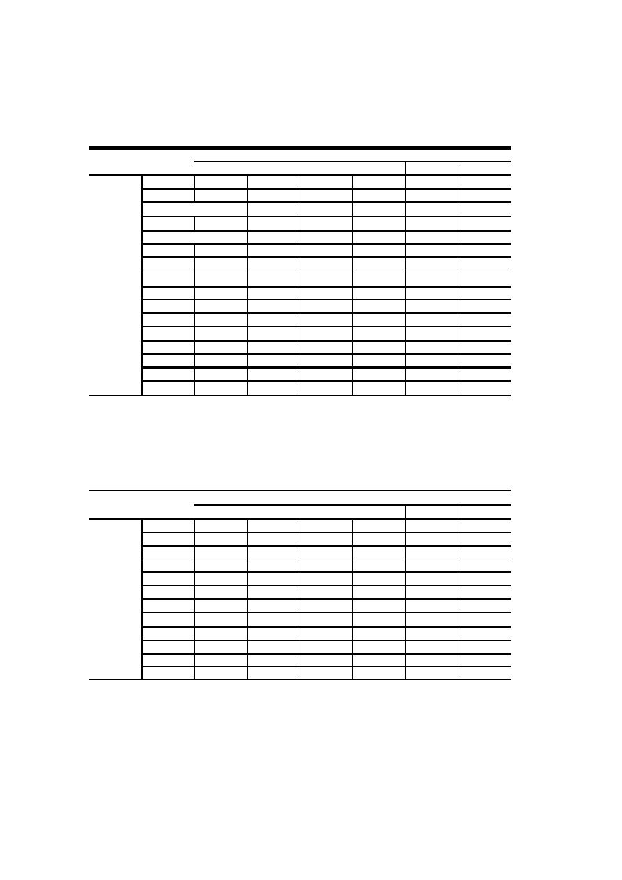
Table 3-1 Matrix of Cumulative Contagion: plots of CC(t,i) of Exchange Rate
1997:1-1999:7

Affected

(nob)

Indonesia

Korea

Malaysia

Philippines

Taiwan

Thailand

ID(61)

0.020

0.145

0.102

0.015

0.133

stat

0.440

4.528

3.049

1.765

5.377

ID till 98/6/17 (49)

0.008

0.180

0.147

0.024

0.157

0.139

4.667

3.900

2.594

5.448

ID after 1998/8/11 (12)

0.063

0.004

-0.079

-0.023

0.038

2.045

0.085

-1.072

-1.146

0.792

KR(14)

0.193

0.124

0.066

0.016

0.215

Origin

stat

1.067

2.643

2.283

0.795

3.593

ML(2)

0.012

0.181

0.233

0.041

0.418

stat

0.024

1.032

1.552

5.490

2.388

PH(3)

-0.089

-0.027

0.186

-0.006

0.173

stat

-0.598

-0.535

1.083

-0.480

1.609

TH(6)

0.107

-0.102

0.047

-0.034

0.043

stat

1.055

-1.051

0.554

-0.708

1.211

TW(1)

0.286

0.218

0.770

0.047

0.552

stat

-

-

-

-

-

Table 3-2 Matrix of Cumulative Contagion: plots of CC(t,i) of Stock Price
Full sample(1994:1-1999:7)

Affected

(nob)

Indonesia

Korea

Malaysia

Philippines

Taiwan

Thailand

ID(30)

0.170

0.276

0.078

0.066

0.187

stat

2.526

3.790

0.687

1.473

2.813

KR(47)

0.011

0.215

0.114

0.031

0.286

stat

0.192

3.731

2.378

0.781

6.181

ML(29)

0.227

0.049

0.276

0.139

0.153

Origin

stat

2.929

0.472

3.752

2.943

2.118

PH(27)

0.266

0.171

0.188

0.076

-0.067

stat

2.543

1.503

2.009

1.310

-0.490

TW(22)

0.074

0.086

0.112

0.124

0.153

stat

1.001

0.874

1.273

1.901

1.885

TH(33)

0.133

0.027

0.062

0.205

0.044

stat

2.204

0.340

0.645

2.850

0.736

45

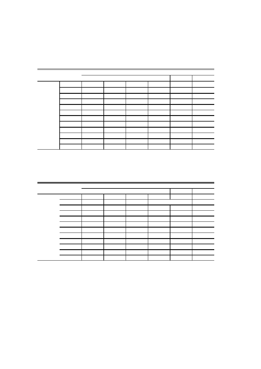
Table 3-3 Matrix of Cumulative Contagion: plots of CC(t,i) of Stock Price
Before Crises (1994:1-1997:6)

Affected

(nob)

Indonesia

Korea

Malaysia

Philippines

Taiwan

Thailand

ID(2)

0.409

0.302

0.556

-0.100

0.182

stat

40.146

1.678

6.543

-0.995

0.685

KR(3)

-0.068

-0.104

-0.086

-0.283

0.127

stat

-0.343

-0.790

-2.549

-2.196

1.275

ML(4)

0.265

-0.123

0.359

0.318

0.254

Origin

stat

3.680

-0.532

2.628

1.974

1.280

PH(12)

0.251

0.095

0.188

0.122

0.261

stat

4.123

0.440

2.321

1.178

2.813

TW(16)

0.013

0.140

-0.025

0.074

0.136

stat

0.289

1.288

-0.267

1.291

1.439

TH(17)

0.155

0.028

0.226

0.122

0.040

stat

2.267

0.341

2.535

1.137

0.532

Table 3-4 Matrix of Cumulative Contagion: plots of CC(t,i) of Stock Price
After Crises (1997:7-1999:7)

Affected

(nob)

Indonesia

Korea

Malaysia

Philippines

Taiwan

Thailand

ID(28)

0.153

0.274

0.044

0.077

0.187

stat

2.152

3.534

0.367

1.660

2.676

KR(44)

0.017

0.237

0.128

0.053

0.297

stat

0.271

3.963

2.525

1.313

6.094

ML(25)

0.222

0.076

0.263

0.111

0.136

Origin

stat

2.469

0.642

3.165

2.326

1.738

PH(15)

0.278

0.232

0.187

0.039

-0.329

stat

5.127

2.352

2.301

0.434

-1.948

TW(6)

0.238

-0.058

0.478

0.256

0.199

stat

1.605

-0.409

1.263

1.901

1.263

TH(16)

0.109

0.026

-0.113

0.293

0.049

stat

1.060

0.185

-0.689

3.144

0.502

46

Table 4-1
Dynamic OLS estimation Results (exchange rate)

origin: all

Affected countries

Indonesia

Korea

Malaysia

Philippines

Taiwan

Thailand

Origin

-0.2745

0.1202

0.1548

0.1977

0.0785

0.1439

replaced s.e.

0.0103

0.0161

0.0111

0.0105

0.5887

0.0089

replaced t

-26.6686

7.4522

13.9628

18.8396

0.1334

16.1375

origin: Indonesia

Affected countries

Indonesia

Korea

Malaysia

Philippines

Taiwan

Thailand

Origin

-0.1135

0.0281

0.0445

0.0203

0.0165

replaced s.e.

0.0634

0.0161

0.0149

0.0021

0.0101

replaced t

-1.7902

1.7451

2.9938

9.9229

1.6350

origin: Korea

Affected countries

Indonesia

Korea

Malaysia

Philippines

Taiwan

Thailand

Origin

0.6754

0.2499

0.2361

-0.0272

-1.4427

replaced s.e.

0.3255

0.0457

0.3633

0.4988

0.2267

replaced t

2.0750

5.4705

0.6499

-0.0545

-6.3648

47

Table 5-1
Dynamic OLS estimation results (stock price)

origin: all full sample

Affected countries

Indonesia

Korea

Malaysia

Philippines

Taiwan

Thailand

Origin

0.4928

-0.0526

0.6497

0.4248

0.0762

0.2526

replaced s.e.

0.0086

0.0108

0.0081

0.0067

0.0034

0.0102

replaced t

57.5051

-4.8807

80.3863

63.5823

22.3790

24.6975

origin: all before crisis

Affected countries

Indonesia

Korea

Malaysia

Philippines

Taiwan

Thailand

Origin

0.0648

-0.2095

-0.1639

0.5348

0.3137

-0.1192

replaced s.e.

0.0107

0.0115

0.0118

0.0227

0.0172

0.0246

replaced t

6.0388

-18.1924

-13.9198

23.5317

18.2456

-4.8500

origin: all after crisis

Affected countries

Indonesia

Korea

Malaysia

Philippines

Taiwan

Thailand

Origin

0.5245

-0.0575

0.6851

0.3867

0.0249

0.2706

replaced s.e.

0.0191

0.0253

0.0162

0.0096

0.0044

0.0152

replaced t

27.5095

-2.2773

42.2091

40.0764

5.6040

17.7667

Table 5-2
Dynamic OLS estimation results (stock price)

origin: Indonesia full sample

Affected countries

Indonesia

Korea

Malaysia

Philippines

Taiwan

Thailand

Origin

-0.0414

1.7127

0.6798

-0.3393

-0.5019

replaced s.e.

0.0411

0.1172

0.5391

0.1836

0.6517

replaced t

-1.0064

14.6173

1.2611

-1.8481

-0.7702

origin: Indonesia after crisis

Affected countries

Indonesia

Korea

Malaysia

Philippines

Taiwan

Thailand

Origin

0.0429

1.7817

0.7583

-0.3861

-0.6235

replaced s.e.

0.0412

0.1170

0.5390

0.1833

0.6504

replaced t

1.0410

15.2293

1.4070

-2.1065

-0.9587

48

Table 5-3
Dynamic OLS estimation results (stock price)

origin: Korea full sample

Affected countries

Indonesia

Korea

Malaysia

Philippines

Taiwan

Thailand

Origin

-0.2442

-0.8312

-4.3166

-0.2285

1.6557

replaced s.e.

0.6812

0.1214

0.6108

0.1174

0.7756

replaced t

-0.3585

-6.8489

-7.0668

-1.9463

2.1347

origin; Korea after crisis

Affected countries

Indonesia

Korea

Malaysia

Philippines

Taiwan

Thailand

Origin

-1.8099

-1.7219

-4.5535

-0.5320

2.1661

replaced s.e.

0.6909

0.1260

0.6500

0.1288

0.8603

replaced t

-2.6196

-13.6701

-7.0049

-4.1305

2.5179

Table 5-4
Dynamic OLS estimation results (stock price)

origin: Malaysia full sample

Affected countries

Indonesia

Korea

Malaysia

Philippines

Taiwan

Thailand

Origin

-1.6294

-0.4216

-0.2906

-0.7256

1.0465

replaced s.e.

0.9864

0.1934

0.8171

0.1355

0.6004

replaced t

-1.6518

-2.1802

-0.3556

-5.3539

1.7428

origin: Malaysia after crisis

Affected countries

Indonesia

Korea

Malaysia

Philippines

Taiwan

Thailand

Origin

-0.9508

-0.3651

-1.7786

-1.2484

1.2640

replaced s.e.

0.9657

0.2273

0.6344

0.1546

0.7342

replaced t

-0.9846

-1.6065

-2.8035

-8.0747

1.7217

49

Table 5-5
Dynamic OLS estimation results (stock price)

origin: Philippines full sample

Affected countries

Indonesia

Korea

Malaysia

Philippines

Taiwan

Thailand

Origin

0.4737

0.6599

1.7336

0.5446

0.1356

replaced s.e.

1.1148

0.0791

0.2248

0.1413

0.8448

replaced t

0.4249

8.3445

7.7120

3.8531

0.1606

origin: Philippines before crisis

Affected countries

Indonesia

Korea

Malaysia

Philippines

Taiwan

Thailand

Origin

5.2982

2.3729

4.1518

0.0599

-3.3578

replaced s.e.

2.8180

0.0329

1.9195

0.3250

11.4663

replaced t

1.8801

72.1742

2.1630

0.1842

-0.2928

origin: Philippines after crisis

Affected countries

Indonesia

Korea

Malaysia

Philippines

Taiwan

Thailand

Origin

0.8472

0.5612

2.2921

0.6950

0.1646

replaced s.e.

0.2302

0.2581

0.2936

0.4977

0.9496

replaced t

3.6797

2.1743

7.8078

1.3965

0.1734

Table 5-6
Dynamic OLS estimation results (stock price)

origin: Taiwan full sample

Affected countries

Indonesia

Korea

Malaysia

Philippines

Taiwan

Thailand

Origin

7.7006

-0.0725

0.9578

-0.5702

2.8019

replaced s.e.

1.5847

0.0243

0.0884

0.4354

1.2694

replaced t

4.8593

-2.9817

10.8287

-1.3095

2.2073

origin: Taiwan before crisis

Affected countries

Indonesia

Korea

Malaysia

Philippines

Taiwan

Thailand

Origin

12.5972

1.2730

2.6296

-4.5437

8.1364

replaced s.e.

0.3443

0.0420

0.0932

0.5978

2.8824

replaced t

36.5889

30.3456

28.2144

-7.6005

2.8228

50

Table 5-7
Dynamic OLS estimation results (stock price)

origin: Thailand full sample

Affected countries

Indonesia

Korea

Malaysia

Philippines

Taiwan

Thailand

Origin

-0.6381

0.8392

1.8733

0.9398

1.3125

replaced s.e.

0.7264

0.0412

0.0992

0.5891

0.1447

replaced t

-0.8785

20.3537

18.8806

1.5953

9.0725

origin: Thailand before crisis

Affected countries

Indonesia

Korea

Malaysia

Philippines

Taiwan

Thailand

Origin

-3.0635

1.2938

2.5083

-0.9537

0.9914

replaced s.e.

1.7643

0.0833

0.4712

0.3671

0.0576

replaced t

-1.7364

15.5275

5.3234

-2.5982

17.2066

origin: Thailand after crisis

Affected countries

Indonesia

Korea

Malaysia

Philippines

Taiwan

Thailand

Origin

0.0540

0.5669

-0.0443

-2.5134

-1.2459

replaced s.e.

2.7935

0.1263

0.1504

0.8779

0.4253

replaced t

0.0193

4.4892

-0.2943

-2.8632

-2.9291

51

Table 6
Export share as a percent of total exports in millions of US dollars.
Selected East Asian countries: 1996-1999

1996

Country

Destination of Exports

Indonesia

Korea

Malaysia

Philippines

Thailand

Japan

US

Indonesia

6.587

2.228

1.381

1.652

25.866

13.641

Korea

2.458

3.351

1.482

2.059

12.336

16.779

Malaysia

1.556

3.046

1.199

4.094

13.403

18.194

Philippines

n.a.

1.818

3.366

3.822

17.973

34.134

Thailand

1.518

1.818

3.614

1.132

16.821

17.993

1997

Country

Destination of Exports

Indonesia

Korea

Malaysia

Philippines

Thailand

Japan

US

Indonesia

6.478

2.539

1.486

1.587

23.361

13.386

Korea

2.601

3.203

1.912

1.650

10.855

15.846

Malaysia

1.556

3.202

1.458

3.644

12.678

18.482

Philippines

0.860

1.752

2.572

3.440

16.856

35.592

Thailand

2.399

1.767

4.327

1.216

15.217

19.436

1998

Country

Destination of Exports

Indonesia

Korea

Malaysia

Philippines

Thailand

Japan

US

Indonesia

5.257

2.780

1.447

1.931

18.662

14.425

Korea

7.015

2.724

2.151

1.097

9.274

17.454

Malaysia

1.376

2.281

1.578

3.161

10.526

21.670

Philippines

0.377

1.730

3.883

2.155

14.388

34.490

Thailand

1.811

1.150

3.269

1.408

13.727

22.357

1999

Country

Destination of Exports

Indonesia

Korea

Malaysia

Philippines

Thailand

Japan

US

Indonesia

7.447

3.282

1.434

2.051

23.571

18.997

Korea

1.754

2.520

2.161

1.199

10.959

20.450

Malaysia

1.458

2.945

1.536

3.266

11.649

21.944

Philippines

0.336

2.822

4.044

2.302

12.741

28.688

Thailand

2.103

1.831

3.891

1.703

15.282

22.772

Notes : Authors' calculation.
Data source: IMF, Direction of Trade, CD-Rom(2000)

52

Table 7
Direct Trade Linkage Index 

1996

Country

Countries export to and import from

Indonesia

Korea

Malaysia

Philippines

Thailand

Indonesia

1.014

0.953

n.a.

0.986

Korea

0.986

1.291

1.677

0.723

Malaysia

1.047

0.709

1.155

1.229

Philippines

n.a.

0.323

0.845

1.106

Thailand

1.014

0.550

0.771

0.894

1997

Country

Countries export to and import from

Indonesia

Korea

Malaysia

Philippines

Thailand

Indonesia

0.989

1.051

1.575

0.762

Korea

1.011

1.267

1.713

0.756

Malaysia

0.949

0.733

1.284

1.072

Philippines

0.425

0.287

0.716

1.102

Thailand

1.238

0.622

0.928

0.898

1998

Country

Countries export to and import from

Indonesia

Korea

Malaysia

Philippines

Thailand

Indonesia

1.180

1.147

1.729

0.978

Korea

0.820

1.366

1.696

0.722

Malaysia

0.853

0.634

1.007

1.131

Philippines

0.271

0.304

0.993

0.905

Thailand

1.022

0.603

0.869

1.095

1999

Country

Countries export to and import from

Indonesia

Korea

Malaysia

Philippines

Thailand

Indonesia

1.176

1.129

1.700

0.896

Korea

0.824

1.189

1.504

0.656

Malaysia

0.871

0.811

0.934

1.096

Philippines

0.300

0.496

1.066

0.917

Thailand

1.104

0.763

0.904

1.083

Notes

: Authors' calculation.

Data source: IMF, Direction of Trade, CD-Rom(2000)

53

Table 8
Imcome Effect  (GDP share, %)

1996
origin

Affected countries

Indonesia

Korea

Malaysia

Philippines

Thailand

Indonesia

0.06128

0.00012

n.a.

0.04571

Korea

0.14430

0.00024

0.04479

0.05474

Malaysia

0.04882

0.08356

0.08294

0.10883

Philippines

0.03026

0.03697

0.00009

0.03410

Thailand

0.03620

0.05135

0.00032

0.09416

1997

origin

Affected countries

Indonesia

Korea

Malaysia

Philippines

Thailand

Indonesia

0.07434

0.00013

0.02602

0.09236

Korea

0.16046

0.00026

0.05301

0.06801

Malaysia

0.06290

0.09152

0.07782

0.16654

Philippines

0.03680

0.05465

0.00012

0.04682

Thailand

0.03930

0.04716

0.00029

0.10408

1998

origin

Affected countries

Indonesia

Korea

Malaysia

Philippines

Thailand

Indonesia

0.05568

0.00014

0.01705

0.08857

Korea

0.27274

0.00023

0.07817

0.05623

Malaysia

0.14423

0.11230

0.17539

0.15989

Philippines

0.07509

0.08867

0.00016

0.06890

Thailand

0.10015

0.04524

0.00032

0.09737

1999

origin

Affected countries

Indonesia

Korea

Malaysia

Philippines

Thailand

Indonesia

0.06239

0.00016

0.01605

0.09882

Korea

0.25647

0.00032

0.13463

0.08603

Malaysia

0.11302

0.08964

0.19294

0.18284

Philippines

0.04940

0.07687

0.00016

0.08000

Thailand

0.07063

0.04264

0.00035

0.10984

Notes : Authors' calculation.
Data source: IMF, Direction of Trade, CD-Rom(2000)

54

Table 9
Cheap Import effect

1996
origin

Affected countries

Indonesia

Korea

Malaysia Philippines Thailand

Indonesia

0.07707

0.00014

n.a.

0.05074

Korea

0.10604

0.00041

0.19835

0.14503

Malaysia

0.03620

0.05773

0.09561

0.19485

Philippines 0.00396

0.01117

0.00008

0.03107

Thailand

0.04816

0.02339

0.00026

0.06942

1997

origin

Affected countries

Indonesia

Korea

Malaysia Philippines Thailand

Indonesia

0.08414

0.00015

0.09399

0.05929

Korea

0.10763

0.00042

0.27906

0.15098

Malaysia

0.04009

0.06302

0.12366

0.20250

Philippines 0.00589

0.01219

0.00009

0.03676

Thailand

0.04019

0.02554

0.00032

0.10518

1998

origin

Affected countries

Indonesia

Korea

Malaysia Philippines Thailand

Indonesia

0.09571

0.00020

0.10106

0.08058

Korea

0.16228

0.00046

0.35217

0.13438

Malaysia

0.06659

0.06890

0.15051

0.19744

Philippines 0.00690

0.02519

0.00019

0.05614

Thailand

0.08943

0.02522

0.00031

0.13024

1999

origin

Affected countries

Indonesia

Korea

Malaysia Philippines Thailand

Indonesia

0.09751

0.00022

0.09197

0.08821

Korea

0.19766

0.00043

0.35522

0.15052

Malaysia

0.09582

0.07753

0.12771

0.21235

Philippines 0.00962

0.02848

0.00021

0.06537

Thailand

0.09561

0.02624

0.00031

0.10723

Notes : Authors' calculation.
Data source: IMF, Direction of Trade, CD-Rom(2000)

55