Geometric Algebra:

Application Studies

Joan Lasenby, Sahan Gamage
and Maurice Ringer
Department of Engineering
University of Cambridge
Trumpington Street
Cambridge, CB2 1PZ, UK
[e-mail]

Chris Doran
Astrophysics Group
University of Cambridge
Madingley Road
Cambridge, CB3 OHE, UK
[e-mail]

http://www-sigproc.eng.cam.ac.uk/vision

http://www.mrao.cam.ac.uk/ clifford

Course Notes to accompany Applications talk: SIGGRAPH 2001, Los

Angeles – Inverse kinematics and dynamics

1

Scope

This set of notes gives some background to the material presented in the applications
lectures. More detail can be found in the references listed at the end of these notes.

The notes cover some of the material presented in the lectures, mainly the inverse kine-
matics and dynamics. The notation follows that in the course although the references
listed adopt a slightly different notation scheme.

1

Tracking, analysis and Inverse Kinematics

1.1

Introduction

The main driving force behind the development of the modelling techniques we will de-
scribe in subsequent sections has been the need to provide fast and efficient algorithms for
optical motion capture. Optical motion capture is a relatively cheap method of producing
3D reconstructions of a subject’s motion over time, the results of which can be used in a
variety of applications; biomechanics, robotics, medicine, animation etc. Using a system
with few cameras (3 or 4) we find that in order to reliably match and track the data (con-
sisting of bright markers placed at strategic points on the subject) we must use realistic
models of the possible motion. Once the data has been tracked using such models, we are
in a position to analyse the motion in terms of the rotors we have recovered.

The mathematical language we will use throughout will be that of geometric algebra
(GA). This language is based on the algebras of Clifford and Grassmann and the form
we follow here is that formalised by David Hestenes [1]. There are now many texts and
useful introductions to GA, [2, 3, 4, 5].

1.2

Rotations

If, in 3D, we consider a rotation to be made up of two consectutive reflections, one in the
plane perpendicular to a unit vector

m

and the next in the plane perpendicular to a unit

vector

n

, it can easily be shown [4] that we can represent this rotation by a quantity

R

we

call a rotor which is given by

R

=

nm

Thus a rotor in 3D is made up of a scalar plus a bivector and can be written in one of the
following forms

R

=

e

B

=2

=

exp

I

2

n

=

cos

2

I

n

sin

2

;

(1)

2

which represents a rotation of

radians about an axis parallel to the unit vector

n

in a

right-handed screw sense. Here the bivector

B

represents the plane of rotation. Rotors act

two-sidedly, ie. if the rotor

R

takes the vector

a

to the vector

b

then

b

=

R aR

y

:

where

R

y

=

mn

is the reversion of

R

(i.e the order of multiplication of vectors in any part

of the multivector is reversed). We have that rotors must therefore satisfy the constraint
that

R R

y

=

1

. One huge advantage of this formulation is that rotors take the same form,

i.e.

R

=

exp (B

)

in any dimension (we can define hyperplanes or bivectors in any

space) and can rotate any objects, not just vectors; e.g.

R (a

^

b)R

y

=

hR abR

y

i

2

=

hR aR

y

R bR

y

i

2

=

R aR

y

^

R bR

y

(2)

gives the formula for rotating a bivector.

Before we leave the topic of rotations, we will outline one property of rotors which will
turn out to be familiar to us from classical Euler angle descriptions of 3D rotations. Con-
sider an orthonormal basis for 3-space,

fe

1

;

e

2

;

e

3

g

; suppose we perform a rotation

R

1

,

where

R

1

=

e

I

1

e

1

, i.e. we first rotate an angle

1

about an axis

e

1

. We then follow this

by a rotation of

2

about the rotated

e

2

axis – this second rotor,

R

2

, is given by

R

2

=

e

I

2

R

1

e

2

R

y

1

The combined rotation is therefore given by

R

T

=

R

2

R

1

– this can be written as follows:

R

T

=

fcos

2

=2

I

R

1

e

2

R

y

1

sin

2

=2

gR

1

=

R

1

fcos

2

=2

I

e

2

sin

2

=2gR

y

1

R

1

=

R

1

R

0

2

(3)

since

R

1

R

y

1

=

1

and

R

1

R

y

1

=

for

a scalar.. Thus if

R

0

2

is the rotation of

2

about

the non-rotated axis (i.e. just

e

2

in this case), we see that the compound rotation can be

written in two ways

R

2

R

1

=

R

1

R

0

2

(4)

Now recall the classical Euler angle formulation: any general rotation can be expressed
as follows: a rotation of

about the

e

3

axis, followed by a rotation of

about the rotated

e

1

axis, followed by a rotation of

about the rotated

e

3

axis [6], as shown in figure 1

Something we always want to do is to apply such a rotation to a vector

x

. In GA terms

we have 3 rotors representing the 3 rotations:

R

1

=

exp f

I

2

e

3

g;

R

2

=

exp f

I

2

e

0

1

g;

R

3

=

exp f

I

2

e

00

3

g

3

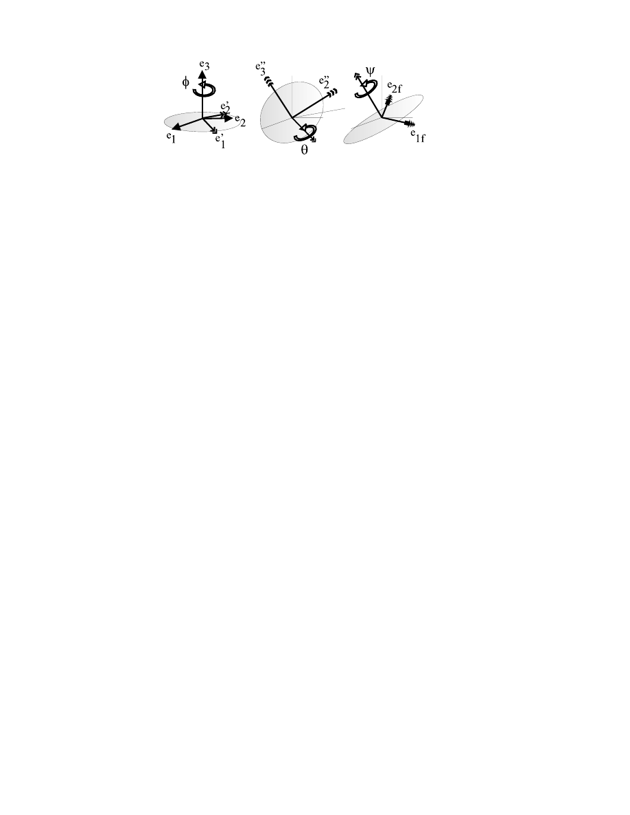
Figure 1: Sketch of the three elementary rotations in the Euler angle formulation – in
which initial axes

(e

1

;

e

2

;

e

3

)

are rotated to final axes

(e

1f

;

e

2f

;

e

3f

)

where

e

0

1

=

R

1

e

1

R

y

1

and

e

00

3

=

R

2

R

1

e

3

R

y

1

R

y

2

. The combined rotor is

R

T

=

R

3

R

2

R

1

so that

x

0

=

R

T

xR

y

T

This is all very straightforward, mainly because we are dealing with active transforma-
tions.

Now, if we implement our Euler angle formulation via rotation matrices, [6], we see that
we have 3 rotations matrices:

A

1

=

cos

sin

0

sin

cos

0

0

0

1

A

2

=

1

0

0

0

cos

sin

0

sin

cos

A

3

=

cos

sin

0

sin

cos

0

0

0

1

which represent the rotations about the non-rotated axes and we apply these matrices in
reverse order to form

A

T

=

A

1

A

2

A

3

so that

x

0

=

A

T

x

If

R

0

1

;

R

0

2

;

R

0

3

are the rotors representing the rotations encoded in

A

1

;

A

2

;

A

3

(i.e. rotations

about the non-rotated axes), then we therefore see that (noting

R

0

1

=

R

1

)

R

0

1

R

0

2

R

0

3

=

R

3

R

2

R

1

which is precisely the formula that we know relates rotations about rotated and non-
rotated axes given in equation 4. Confusion often arises due to the passive nature of
the Euler angle formulation as given in standard textbooks – there is no such confusion
possible if we work totally with active transformations, as one is forced to do with the
rotor formulation.

1.3

Articulated Motion Models: Forward Kinematics and Tracking

We begin by considering a simple model of a leg as two linked rigid rods shown in fig-
ure 2. Let us assume that the first rod,

AB

, can rotate with all degrees of freedom about

4

Figure 2: Two linked rigid rods used to simulate the leg

point

A

but that the second rod,

B

C

, can only rotate in the plane formed by the two

rods (i.e. about an axis which is perpendicular to both rods and initially aligned with the

e

2

axis). In reality more complex constraints can be considered.

e

1

;

e

2

;

e

3

form a fixed

orthonormal basis oriented as shown.

x

a

;

x

b

;

x

c

are the vectors representing the 3D posi-

tions of

A;

B

;

C

respectively and

x

1

=

x

b

x

a

and

x

2

=

x

c

x

b

, which, initially, take

the values

d

1

e

1

and

d

2

e

1

. We can immediately write down the position of points

B

and

C

as

x

b

=

x

a

+

d

1

R

1

e

1

R

y

1

(5)

x

c

=

x

b

+

d

2

R

2

R

1

e

1

R

y

1

R

y

2

(6)

where we have

R

1

=

exp f

I

1

2

n

1

g

and we allow for the fact that the point

A

may move

in space (note here that we allow any rotation of rod

AB

about

A

, although we may want

to only have 2 dof rather than 3 if we are not interested in the orientation of the axes
at

A

). We also have that

R

2

=

exp f

I

2

2

n

0

2

g

with

n

0

2

=

R

1

e

2

R

y

1

. Using the fact that

R

2

R

1

=

R

1

R

0

2

with

R

0

2

=

exp f

I

2

2

e

2

g

we are able to give the position of the ankle,

x

c

as

x

c

=

x

a

+

d

1

R

1

e

1

R

y

1

+

d

2

R

1

R

0

2

e

1

R

y

0

2

R

y

1

x

a

+

R

1

fd

1

e

1

+

d

2

R

0

2

e

1

R

y

0

2

gR

y

1

(7)

Thus we are able to write down, in a manner which deals only with active transformations,
such forward kinematics equations for arbitrarily complex mechanisms. But this is not the
only advantage of this approach; we can now have the elements of our state as rotors – it
is well known that singularities can occur using Euler angles (i.e. when an angle goes to
zero,

90

Æ

or other specific ranges) and we can avoid many of these singularities using the

rotor components as our variables. The use of such models in optical tracking scenarios
is briefly discussed here.

In a typical multi-camera tracking problem where we place markers on joints, the mea-
surements (2D points in the camera planes) will be related to the state via a measurement
equation:

y

(k

)

=

H

k

(x

(k

))

+

w

(k

)

(8)

5

where the

y

(k

)

is our set of measurements (observations) at time

t

=

k

,

x

(k

)

is the state at

time

t

=

k

(parameters describing our model(s)), and

w

(k

)

is a zero-mean random vector

representing noise at the detection points. The function

H

k

relates the model parameters

to the observations. In this case we take our model parameters to be the coefficients of the
bivectors representing the rotors (

B

=

b

1

I

e

1

+

b

2

I

e

2

+

b

3

I

e

3

) and then use expressions

such as equation 7 to relate these to our observations.

The process equation

x(k

+

1)

=

F

k

(x

(k

))

+

v

(k

)

tells us how our system (model) evolves in time; here

v

(k

)

represents the process noise.

In the case described,

F

k

tells us how we believe the bivectors to be evolving – one might

argue that the variation of the bivectors will be smoother than the evolution of separate
Euler-angles.

In general,

H

k

will be extremely non-linear and so the above problem can be solved by

applying an extended Kalman filter (EKF) to update our model estimates and predicted
observations at each time step.

A detailed comparison of the difference between using Euler-angles and using bivector
coefficients as the scalar model parameters in such tracking problems will be given else-
where.

1.4

Inverse kinematics (IK)

Inverse kinematics is the procedure of recovering the model or state parameters given the
measurements – in particular, when incomplete sets of measurements are given (i.e. not
all the joint coordinates) we can, in certain cases, recover a unique model or a specified
family of solutions. In this section we shall outline the use of GA in solving IK problems
by consideration of a particular, fairly simple, example. The example we choose is the
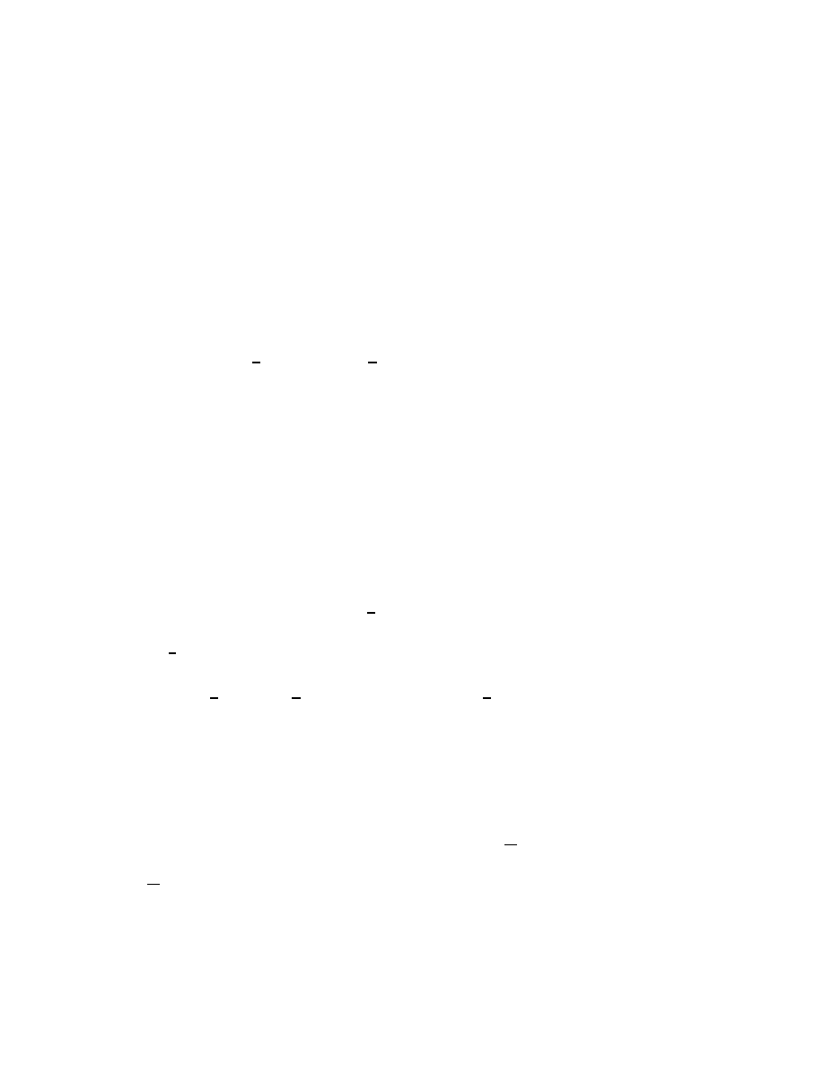
following (it is one which often appears in standard texts); a system consisting of three
linked rigid rods representing a typical insect leg – such a setup is commonly used in
walking robots and is illustrated in figure 3. Here we fix a set of axes represented by unit
vectors

(e

1

;

e

2

;

e

3

)

(note that in the figure,

e

1

;

e

2

;

e

3

are shown) at the basal joint, so

that the angle of the first link, or coxa, is given by the Euler angles

(

;

;

)

, and the rotor

representing this rotation is

R

A

=

e

I

2

e

3

e

I

2

e

1

e

I

2

e

3

R

R

R

(9)

Generally the angles

(;

)

are taken as known, so that

alone describes the position of

the first link. The second (femur) and third (tibia) links are such that only rotation in the
plane of the three links is allowed, so that the positions of the leg are fully described by

6

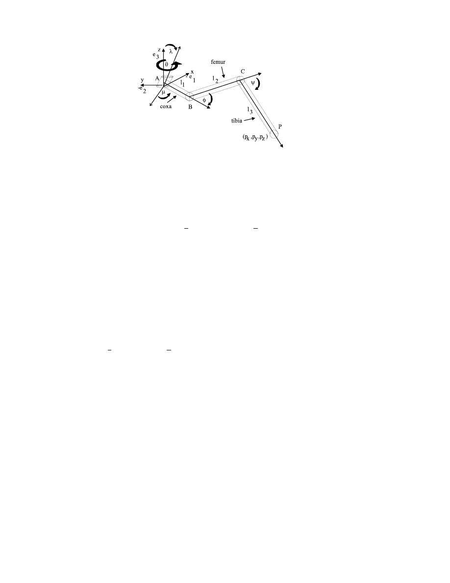
Figure 3: Three linked rigid rods representing the leg of an insect

two further angles,

and

as shown in figure 3. If we take our initial configuration to

be that in which the leg is fully extended with all links lying along the rotated (by

R

A

)

e

2

direction (i.e.

and

=

0

), then the rotations at joints

B

and

C

are given by

R

B

=

e

I

2

e

0

1

and

R

C

=

e

I

2

e

00

1

(10)

where

e

0

1

=

R

A

e

1

R

y

A

;

e

00

1

=

R

B

R

A

e

1

R

y

A

R

y

B

. Note here that we are rotating about the

e

1

direction in order to give the sense of

and

shown in figure 3. We are thus able to

write down the postion vectors of all joints and finally of the foot position

x

P

as follows

x

B

=

x

A

+

R

A

(

l

1

e

2

)R

y

A

R

R

R

(

l

1

e

2

)R

y

R

y

R

y

(11)

x

C

=

x

B

+

R

B

R

A

(

l

2

e

2

)R

y

A

R

y

B

=

x

B

+

R

A

R

0

B

(

l

2

e

2

)R

y

0

B

R

y

A

(12)

x

P

=

x

C

+

R

C

R

B

R

A

(

l

3

e

2

)R

y

A

R

y

B

R

y

C

=

x

C

+

R

A

R

0

B

R

0

C

(

l

3

e

2

)R

y

0

C

R

y

0

B

R

y

A

(13)

where

R

0

B

=

e

I

2

e

1

and

R

0

C

=

e

I

2

e

1

. We can therefore write

x

P

as

x

P

=

x

A

+

R

A

f

l

1

e

2

+

R

0

B

f

l

2

e

2

+

R

0

C

(

l

3

e

2

)R

y

0

C

gR

y

0

B

gR

y

A

(14)

This uniquely gives the forward kinematic equations in terms of the three rotors

R

A

;

R

B

;

R

C

;

if one was to convert this to angles one gets the following equations (which are conven-
tionally obtained when one uses transformation matrices to denote position of one joint
relative to the previous joint [7]):

p

x

=

(cos

cos

~

cos

sin

sin

~

)[l

2

cos

+

l

3

cos (

+

)

+

l

1

]

+

sin

sin

[l

2

sin

+

l

3

sin

(

+

)]

p

y

=

(sin

cos

~

+

cos

cos

sin

~

)[l

2

cos

+

l

3

cos (

+

)

+

l

1

]

(15)

sin

cos

[l

2

sin

+

l

3

sin

(

+

)]

p

z

=

sin

sin

~

[l

2

cos

+

l

3

cos (

+

)

+

l

1

]

+

cos

[l

2

sin

+

l

3

sin(

+

)]

7

In the above,

~

=

=2

, since the convention (following Denavit-Hartenberg) is to

measure this basal rotation angle from the

e

2

axis rather than from the

e

1

axis as our rotor

formulation has done. Now, the inverse kinematics comes in when we try to recover the
joint angles

(

~

;

;

)

given

(p

x

;

p

y

;

p

z

)

(and the origin of coordinates). Conventionally

the solution is obtained by a series of fairly involved matrix manipulations to give the
following expressions for the joint angles:

~

=

arctan

p

x

cos

sin

+

p

y

cos

cos

+

p

z

sin

p

x

cos

+

p

y

sin

=

arctan

0

@

s

1

z

2

+

x

2

+

y

2

l

2

2

l

2

3

2l

2

l

3

2

=

z

2

+

x

2

+

y

2

l

2

2

l

2

3

2l

2

l

3

1

A

=

arctan

z

x

2

+

y

2

arctan

l

3

sin

l

2

+

l

3

cos

(16)

where

x

=

p

x

cos

+

p

y

sin

l

1

cos

~

(17)

y

=

p

x

cos

sin

+

p

y

cos

cos

+

p

z

sin

l

1

sin

~

(18)

z

=

p

x

sin

sin

p

y

sin

cos

+

p

z

cos

(19)

In standard texts it is often noted that it is better to express joint angles in terms of arctangent
functions to avoid quadrant polarities – we will return to this point later when discussing problems
with this Euler angle formulation. Suppose that we have the points

x

a

;

x

b

;

x

c

;

x

p

, we will now

show that it is straightforward, from equations 11-13, to recover each of the rotors,

R

A

;

R

B

;

R

C

.

In order to do this we shall use a simple result from GA (see [4] for more details). Suppose that a
set of three (non-coplanar and not necessarily orthonormal) unit vectors

e

1

;

e

2

;

e

3

is rotated by a

rotor

R

into a set of three other (necessarily non-coplanar) unit vectors

f

1

;

f

2

;

f

3

– then the unique

rotor which performs this job is given by

R

/

1

+

e

i

f

i

(20)

where the proportionality factor is easily found by ensuring

R R

y

=

1

and

fe

i

g

denotes the recip-

rocal frame of

fe

i

g

. The reciprocal frame

fe

i

g

is such that

e

i

e

j

=

Æ

i

j

and can be formed (for 3D)

as follows

e

1

=

1

I

e

2

^

e

3

e

2

=

1

I

e

3

^

e

1

(21)

e

3

=

1

I

e

1

^

e

2

;

(22)

where

I

=

e

3

^

e

2

^

e

1

.

This provides us with a remarkably easy way of extracting rotors if we know the joint coordinates.
Let us first consider equation 11 for

R

A

. We can rewrite this equation as

R

y

R

y

(x

B

x

A

)R

R

=

R

(

l

1

e

2

)R

y

(23)

8

From this we can see that the vector

f

1

=

l

1

e

2

is rotated into the vector

g

1

=

R

y

R

y

(x

B

x

A

)R

R

and also that, since

R

=

e

I

1

2

e

3

, the vector

f

2

=

e

3

is rotated into itself, i.e.

g

2

=

e

3

.

From this it follows that

f

3

=

I

f

1

^

f

2

must be rotated into

g

3

=

I

g

1

^

g

2

. Thus, using equations 22

we can form

ff

i

g

and the rotor

R

as follows

R

/

1

+

f

i

g

i

where

[f

1

;

f

2

;

f

3

]

=

[

l

1

e

2

;

e

3

;

I

f

1

^

f

2

]

and

[g

1

;

g

2

;

g

3

]

=

[R

y

R

y

(x

B

x

A

)R

R

;

e

3

;

I

g

1

^

g

2

]

(24)

Thus

R

A

is then recovered from equation 9. Using this we can now look at equation 12 which can

be rewritten as

R

y

A

(x

C

x

B

)R

A

=

R

0

B

(

l

2

e

2

)R

y

0

B

(25)

We can then invert as above to give

R

0

B

/

1

+

f

i

g

i

where

[f

1

;

f

2

;

f

3

]

=

[

l

2

e

2

;

e

1

;

I

f

1

^

f

2

]

and

[g

1

;

g

2

;

g

3

]

=

[R

y

A

(x

C

x

B

)R

A

;

e

1

;

I

g

1

^

g

2

]

(26)

Finally,

R

0

C

can be recovered by precisely the same means using

R

0

C

/

1

+

f

i

g

i

where

[f

1

;

f

2

;

f

3

]

=

[

l

3

e

2

;

e

1

;

I

f

1

^

f

2

]

and

[g

1

;

g

2

;

g

3

]

=

[R

y

0

B

R

y

A

(x

P

x

C

)R

A

R

0

B

;

e

1

;

I

g

1

^

g

2

]

(27)

Thus, we see that we are able to invert our forward kinematic equations trivially if we have the
coordinates of the joints. Of course, the IK problem as we described it involved being given only

x

A

and

x

P

. The plan we advocate is therefore to find

x

B

and

x

C

by purely geometric means as an

initial stage, followed by the rotor inversion process described above. To illustrate this, consider
how we would find

x

B

;

x

C

for the given example.

Taking

x

A

at the origin, we know that

e

0

3

and

x

P

must define the plane in which all the links must

lie, call this plane

– see figure 4. We can form

x

B

via

x

B

=

l

1

(x

p

(x

P

e

0

3

)e

0

3

)

jx

p

(x

P

e

0

3

)e

0

3

j

(28)

There are clearly two possibilities for

x

C

, given by the intersections of the circles lying in the

plane

having centres and radii given by

(x

B

;

l

2

)

and

(x

P

;

l

3

)

. If we then define

e

k

=

(x

P

x

B

)=(jx

P

x

B

)j

and

e

?

a vector perpendicular to

e

k

lying in

, it is not hard to show that

x

C

is

given by

x

C

=

x

k

e

k

+

x

?

e

?

where

x

k

=

l

2

2

l

2

3

+

(x

P

x

B

)

2

2jx

P

x

B

j

(29)

x

2

?

=

[(l

2

l

3

)

2

(x

P

x

B

)

2

][(l

2

+

l

3

)

2

(x

P

x

B

)

2

]

4jx

P

x

B

j

(30)

9

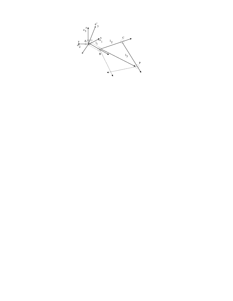
Figure 4: Figure illustrating setup used to determine joint positions from geometry

When the geometry is more complex than given in this example (indeed, things will get more com-
plicated if we also have prismatic joints rather than simple revolute joints) the joint positions, or
family of joint positions are found by intersecting circles, spheres, planes and lines (with possible
dilations) in 3D. The system that we are currently working on performs this initial geometric stage
in the 5D conformal geometric algebra [8, 9]. This framework provides a very elegant means of
dealing with incidence geometry and extends the functionality of projective geometry to include
circles and spheres. A feature of the conformal setting is that rotations, translations, dilations and
inversions in 3D all become rotors in 5D.

We now return to the question of whether we gain any advantages from doing our IK problems
in geometric algebra. In the simple case illustrated, simulations have shown that we can recover
the rotors (there always exist two sets of solutions) exactly for any combination of angles – there
is no need to restrict any of the angles to particular ranges. However, when the equations in 16
are used to recover angles, we find that the whole process is plagued with conditionals, i.e. the
correct solutions are obtained only if signs of various terms are checked for various angles in
various ranges. From a computing point of view this is expensive and may ultimately lead to
hard-to-track-down errors.

1.5

Conclusions

Here we have illustrated how the geometric algebra, and particularly the rotor formulation within
the algebra, can be used as a mathematical system in which forward kinematics, motion modelling
and inverse kinematics can be elegantly expressed. The formulations given have been put to use
in tracking problems in which optical motion capture data is tracked via constrained articulated
models and in inverse kinematics of simple leg structures. We believe that the system as outlined
here has enormous potential in more complex inverse kinematics problems where we would like
to define families of possible solutions – the key here would be to do the initial geometry stage via
a 5D conformal geometric algebra. Work in progress also includes the analysis of human motion
data via our articulated models in an attempt to understand how motions are described using the
rotor formulation.

10

2

Inferring dynamical information from 3D position data
using geometric algebra

2.1

Introduction

Estimating inverse dynamic (ID) quantities is essential in areas such as robot control, biomedical
engineering and animation. In the field of robotics there are numerous techniques and procedures
for calculating these quantities [10, 11]. The computational procedure given in [11] for estimat-
ing ID quantities is the Luh-Walker-Paul algorithm [12]. Also in the context of estimating ID
quantities from marker data, [13] has presented an inertial model and a method to calculate the
joint moments, although this is not an explicit algorithm for calculation of these quantities. Here
we present a step-by-step algorithm to estimate the ID quantities using only the 3D positions of
markers attached to an articulated body in general motion using Geometric Algebra (GA). The
simplicity of the derivations given here is due to the fact that the rotation of a body is represented
as a single quantity; namely the rotational bivector. When Euler angles are used to model the
rotation it is extremely difficult to formulate the ID quantities in a simple manner. Using the stan-
dard technique of employing angular velocity vectors [11, 13] does not yield a simple connection
between the rotational quantities and the actual ID parameters. In such formulations it is not clear
how to obtain the angular velocity vector in numerical calculations when the axis and the angle of
rotation change with time. Since the direction and the magnitude of rotation are incorporated into
a single quantity when rotational bivectors are used, each kinematic and dynamic parameter can
be expressed directly.

First we present the basic formulation of the dynamic equations in GA and then derive the angular
velocity and acceleration bivectors given the rotations. Then we adapt these results for calculations
with marker data. We apply the techniques to real world data obtained from an experimental setup
of a person walking on a moving bridge.

2.2

Some Basic Formulations

Here we either derive or state some basic formulae needed for the calculation of inverse dynamics.

2.3

Angular Velocity

If set of vectors

f f

k

g

on a body rotating in space can be related to a fixed time independent set of

corresponding vectors

fe

k

g

by a time dependent rotor

R

, we can write

f

k

=

R e

k

R

y

.

(31)

Define the angular velocity bivector of the rotating system [14, 15] in space,

s

, via the equation

_

f

k

=

S

f

k

(32)

11

where operator

denotes the commutator product defined as

A

B

=

B

A

=

(AB

B

A)

=2

and

_

f

k

are the velocity vectors. This is analogous to the ‘conventional’ definition of

_

f

k

=

!

x

f

k

where x denote the vector cross product and

!

is the angular velocity vector which is related to

S

by

S

=

I

!

[14] with

I

being the pseudoscalar in 3D. Equation (31) can be differentiated with

respect to (wrt) time to give

_

f

k

=

_

R e

k

R

y

+

R e

k

_

R

y

.

(33)

Note that

_

e

k

=

0

since

e

k

is fixed. But since

R R

y

=

1

,

_

R R

y

+

R

_

R

y

=

0

, and therefore

_

R

y

=

R

y

_

R R

y

.

(34)

Equation (33) can then be re-arranged as

_

f

k

=

2

_

R

R

y

f

k

. It can be proved [14] that the quantity

_

R R

y

is a bivector. Hence we can associate it with the angular velocity bivector of equation (32);

S

=

2

_

R R

y

(35)

and thus

_

f

k

=

f

k

S

. It is also possible to rearrange equation (35) to give

_

R

=

1

2

S

R

.

(36)

The angular velocity referred back to the body,

B

, is the ‘body’ angular velocity and is defined

[14, 15] by

S

=

R

B

R

y

.

(37)

2.3.1

Linear Velocity, Acceleration and inertial force

In general the points on a rigid body which is in general motion relative to a measuring coordinate
system can be expressed as

y

i

=

R x

i

R

y

+

d

(38)

where

y

i

and

d

are the

i

th point and the displacement of the Centre of Mass (CoM) of the body in

the observation frame respectively.

x

i

is the

i

th point referred to a conveniently chosen fixed set

of axes on the body placed at the CoM. Hence,

x

i

has no time dependence assuming rigidity of

the body. Differentiating equation (38) wrt to time gives the velocity of the point on the body in
the observation frame

_

y

i

as

_

y

i

=

_

R x

i

R

y

+

R x

i

_

R

y

+

_

d

.

Using equations (34) and (35) it is possible to derive (see for e.g. [16]),

_

y

i

=

(y

i

d)

S

+

_

d

R x

i

R

y

S

+

_

d

.

(39)

Differentiating equation (39) wrt to time again and substituting for

(

_

y

i

_

d)

gives the acceleration

as



y

i

=

(y

i

d)

_

S

+

[(y

i

d)

S

]

S

+



d

.

Hence using Newton’s second law, the inertial force,

F

, acting on the body can be written as

F

=

m



y

i

where

m

is the mass of the body if the observation frame is an inertial (constant velocity) frame

of reference.

12

2.3.2

Angular momentum, inertia tensor and inertial torque

It is straightforward to derive the angular momentum bivector,

L

, of a body. In [14] it is shown to

be given by

L

=

R I

(

B

)R

y

with

I

(B

)

=

Z

d

3

xx

^

(x

B

)

(40)

where

I

(:)

is a linear mapping of bivectors onto bivectors, and is the inertia tensor of the body.

Since the inertia tensor is an integration referred to the ‘fixed’ copy vectors, it is time independent.
But note that

B

is time dependent. Inertial torque,

, satisfies

=

_

L

and we can form

_

L

by

differentiating equation (40) wrt time to give

_

L

=

_

R I

(

B

)R

y

+

R I

(

B

)

_

R

y

+

R I

(

_

B

)R

y

.

But using equation (34)

_

L

can be expressed ([14, 16]) as

_

L

=

1

2

S

R I

(

B

)R

y

+

1

2

R I

(

B

)R

y

S

+

R I

(

_

B

)R

y

.

Hence from equation (37), inertial torque is given as ([14, 16]),

=

_

L

=

R

h

I

(

B

)

B

+

I

(

_

B

)

i

R

y

.

(41)

2.4

Calculations in terms of rotational bivectors

Here we present a method to calculate the angular velocity bivector

S

and the angular accel-

eration bivector

_

S

given only the rotational bivector

B

. The derivation of

S

is similar to the

method presented in [17]. First we use the definition of the rotor

R

in terms of the bivector

B

R

exp

(

B

)

exp(

2

^

B

)

cos (

=2)

sin

(

=2)

^

B

(42)

where

B

=

2

^

B

and

^

B

2

=

1

, to evaluate

_

R

=

_

2

sin

(

=2)

_

2

cos (

=2)

^

B

sin

(

=2)

_

^

B

=

_

2

^

B

R

sin

(

=2)

_

^

B

.

Hence we can write

S

=

2

_

R R

y

in terms of the above as

S

=

_

^

B

+

2

sin

(

=2)

_

^

B

R

y

.

(43)

Since it is easier to evaluate

_

B

than

_

^

B

and

_

, it makes sense to write

_

and

_

^

B

in terms of

_

B

2

=

4B

B

,

2

_

=

4

_

B

B

4B

_

B

,

_

=

4

_

B

B

=

(44)

where

AB

=

( AB

+

B

A)

=2

is the anti-commutator product. Since

^

B

=

2B

=

and therefore

^

B

=

2B

, we have

_

^

B

+

_

^

B

=

2

_

B

=

)

_

^

B

=

2

_

B

_

^

B

=

.

(45)

13

Note that the formulae for

_

and

_

^

B

in [17] are incorrect due to an error in defining equation (42):

in [17]

B

is taken as

^

B

rather than

2

^

B

. All subsequent derivations in [17] are correct if we

substitute

j B

j

for

.

In order to evaluate the angular acceleration,

_

S

, in terms of

,

B

,

_

B

and



B

, we differentiate

equation (43) wrt time and substitute from equation (34) for

_

R

y

to give

_

S

=



^

B

+

_

_

^

B

+

_

cos(

=2)

_

^

B

R

y

+

2

sin

(

=2)



^

B

~

R

+

sin

(

=2)

_

^

B

R

y

S

(46)

Here,



and



^

B

are to be evaluated. Differentiating equations (44) and (45) gives



=

4



B

B

+

4

_

B

2

+

_

2

=

and



^

B

=

2



B



^

B

2

_

_

^

B

=

Also via equation (37), it is possible to derive the relationship between

_

B

and

_

S

as

_

B

=

R

y

_

S

R

.

(47)

A complete derivation of all the above basic results can be found in [16].

Also, as a first approximation, we use the two sided Euler formulae for the numerical derivatives
but if higher accuracy is needed, especially in the noisy data case, a polynomial fit for the function
around each data point can be used. A sophisticated realisation of this is the Savitzky-Golay filters
as implemented in [18].

3

Algorithm for Inverse Dynamics

Here we describe an algorithm for calculating inertial forces and torques given only the marker
positions attached to an articulated model using results from previous sections. The assumptions
are;

1. the 3D marker coordinates (possibly noisy) at each time instance are given

2. the time intervals for the data sets are known or constant

3. markers are labelled in the sense that it is known a priori to which link a marker is attached

4. each link can be modelled as a rigid body, attached either to a ball or a hinge joint.

5. the principal axes of inertia for each link in the observation coordinate frame are known

6. the centre of mass (CoM) in relation to the joint location is known.

Hence each marker position can be expressed as

R

k

(l

)e

p

r

(l

)R

y

k

(l

)

+

t

k

=

v

p

k

(l

)

(48)

14

where

R

k

(l

)

is the rotation at the

k

th time instance of the

l

th link relative to a given observation

reference coordinate frame. Also

e

p

r

(l

)

is the vector from the joint to the

p

th marker at the

r

th time

instance (usually we take

r

=

1

),

t

k

is the translation vector of the joint relative to the observation

reference frame.

Under the assumptions given above, the inertial forces and torques can be calculated by the fol-
lowing algorithm;

1. estimate the joint locations

t

k

, for all time instances

2. estimate the link rotations,

R

k

(l

)

, relative to the coordinate system at the first time instance,

for all time instances and for all links

3. calculate the vector from a joint to its CoM,

c

k

(l

)

, for all time instances.

4. calculate the total rotation from the principal axes of inertia to the current observation,

R

T

k

(l

)

, for each link at each time instance

5. calculate the corresponding rotational bivector

B

T

k

(l

)

at each time instance and for each

link

6. estimate the

_

B

T

k

(l

)

and hence calculate inertial forces and torques.

Using the techniques described in [19], it is possible to estimate

t

k

and

R

k

(l

)

in a least squares

sense. When there is a hierarchical kinematic chain, the local averaging global method in [19]
can be used. In that method the positions of the joints are built up from considering only one joint
at a time and averaging the results over the common links between joints.

Then the position vector from the CoR in the case of a ball joint and the perpendicular distance
from the AoR in the case of a hinged joint,

c

k

(l

)

, can be calculated if the relative location of the

CoM to the joint is known (e.g. middle of the link).

If the rotation required to bring the principal axes of inertia for each link to the observation frame,

r

r

(l

)

, is known (assumption 5), the total rotation of the principal axes can be expressed as

R

T

k

(l

)

=

R

k

(l

)r

r

(l

)

.

Hence

B

T

k

(l

)

can be estimated from

R

T

k

(l

)

=

exp

B

T

k

(l

)

.

(49)

3.1

Dynamical Equilibrium in the model

In a system that has one or several articulated chains connected to a central body, equilibrium
of the central body can be calculated by working from the bottom of the articulated hierarchy
and transferring forces up to the central body. This is also the foundation of Luh-Walker-Paul’s

15

algorithm [12]. Considering the free body diagram for a single link the forces acting on the link
can be expressed as

F

v

k

(l

)

F

v

k

(l

+

1)

+

m(l

)g

=

m(l

)



y

v

k

(l

)

(50)

where

F

v

k

(l

)

is the force vector acting on the joint at the beginning of the link

l

on the

v

th kinematic

chain at the

k

th time instance,

F

v

k

(l

+

1)

is the force vector acting on the joint at the beginning

of the link

l

+

1

on the

v

th kinematic chain at the

k

th time instance,

m(l

)

the mass of the link

l

,

g

the gravitational pull per unit mass and



y

v

k

(l

)

is the acceleration of the CoM. Writing the set of

equations for the link

L

v

down to link

1

where

L

v

is the last link of the

v

th chain, we have

F

v

k

(1)

=

F

v

k

(L

v

+

1)

+

L

v

X

l =1

m(l

)



y

v

k

(l

)

L

v

X

l =1

m(l

)g

(51)

where

F

v

k

(L

v

+

1)

is taken to be the external force acting at the end of link

L

v

. Considering the

equilibrium of the central body gives

V

X

v

=1

F

v

k

(1)

=

m(b)



y

b

k

(52)

assuming

V

chains are connected to the central body

b

. Hence substituting for

F

v

k

(1)

in equation

(52) from equation (51) gives

V

X

v

=1

F

v

k

(L

v

+

1)

=

V

X

v

=1

L

v

X

l =1

m

v

(l

)g

V

X

v

=1

L

v

X

l =1

m

v

(l

)

d.

ot

y

v

k

(l

)

m(b)



y

b

k

(53)

An analogous torque relationship can be derived by considering the torque acting on the CoM of
each link giving the final equilibrium equation as

V

X

v

=1

T

v

k

(L

v

+

1)

=

V

X

v

=1

L

v

X

l =1

v

k

(l

)

b

k

.

(54)

The full derivation is given in [16]. As for the forces,

T

v

k

(L

v

+

1)

is the external torque acting

on the

L

v

th link.

3.2

Inverse Dynamics from Motion Capture Data

Assuming the location of the CoM, the principal axes of inertia of each link and the 3D marker
positions attached to the links, it is possible to calculate the inertial force and torque quantities
relating to the subject of the motion capture. Assuming the frame rate of the capture system
is constant with an interval of

P

, given the bivectors

B

T

k

+1

(l

)

,

B

T

k

(l

)

,

B

T

k

1

(l

)

, the translations

t

k

+1

(l

)

,

t

k

(l

)

,

t

k

1

(l

)

and the

c

k

(l

)

, the results in the previous sections can be summarised as;

_

B

T

k

(l

)

B

T

k

+1

(l

)

B

T

k

1

(l

)

2P

,



B

T

k

(l

)

B

T

k

+1

(l

)

2B

T

k

(l

)

+

B

T

k

1

(l

)

P

2



t

k

(l

)

t

k

+1

(l

)

2t

k

(l

)

+

t

k

1

(l

)

P

2

k

(l

)

=

2

q

B

T

k

(l

)B

T

k

(l

)

,

^

B

T

k

(l

)

=

2B

T

k

(l

)

k

(l

)

16

_

k

(l

)

=

4

_

B

T

k

(l

)B

T

k

(l

)

k

(l

)

,

_

^

B

T

k

(l

)

=

2

_

B

T

k

(l

)

_

k

(l

)

^

B

T

k

(l

)

k

(l

)

S

k

(l

)

=

_

k

(l

)

^

B

T

k

(l

)

+

2

sin

(

k

(l

)=2)

_

^

B

T

k

(l

)R

y

k

T

(l

)



k

(l

)

=

0

B

@

4



B

T

k

(l

)B

T

k

(l

)

+

4

_

B

T

k

(l

)

2

+

_

k

(l

)

2

k

(l

)

1

C

A



^

B

T

k

(l

)

=

2



B

T

k

(l

)



k

(l

)

^

B

T

k

(l

)

2

_

k

(l

)

_

^

B

T

k

(l

)

k

(l

)

_

S

k

(l

)

=



k

(l

)

^

B

T

k

(l

)

+

_

k

(l

)

_

^

B

T

k

(l

)

+

_

k

(l

)

cos (

k

(l

)=2)

_

^

B

T

k

(l

)R

y

k

T

(l

)

+

2

sin

(

k

(l

)=2)



^

B

T

k

(l

)R

y

k

T

(l

)

+

sin

(

k

(l

)=2)

_

^

B

T

k

(l

)R

y

k

T

(l

)

S

k

(l

)



c

k

(l

)

=

c

k

(l

)

_

S

k

(l

)

+

c

k

(l

)

S

k

(l

)

S

k

(l

)

(55)

F

k

(l

)

=

m(l

)



c

k

(l

)

+



t

k

(l

)

B

k

(l

)

=

R

y

k

T

(l

)

S

k

(l

)R

T

k

(l

)

,

_

B

k

(l

)

=

R

y

k

T

(l

)

_

S

k

(l

)R

T

k

(l

)

k

(l

)

=

R

T

k

(l

)

h

I

(

B

k

(l

))

B

k

(l

)

+

I

(

_

B

k

(l

))

i

R

y

k

T

(l

)

(56)

where

S

k

(l

)

and

B

k

(l

)

are the ‘space’ and ‘body’ angular velocity bivectors respectively.

If the data from the whole system is available it is possible to apply the equilibrium equations (53)
and (54) to estimate the external forces and torques acting on the system up to a scale factor using

V

X

v

=1

F

v

k

(L

v

+

1)

=

V

X

v

=1

L

v

X

l =1

m

v

(l

)g

V

X

v

=1

L

v

X

l =1

m

v

(l

)



c

v

k

(l

)

+



t

v

k

(l

)

m(b)

h



c

b

k

+



t

b

k

i

and

V

X

v

=1

T

v

k

(L

v

+

1)

=

V

X

v

=1

L

v

X

l =1

k

(l

)

b

k

where



c

v

k

(l

)

and



c

b

k

are evaluated from equation (55) and

k

(l

)

and

b

k

are evaluated using equation

(56). Note that



c

v

k

(l

)

+



t

v

k

(l

)

is the acceleration of the CoM of the

l

th link at time

k

of the branch

v

.

4

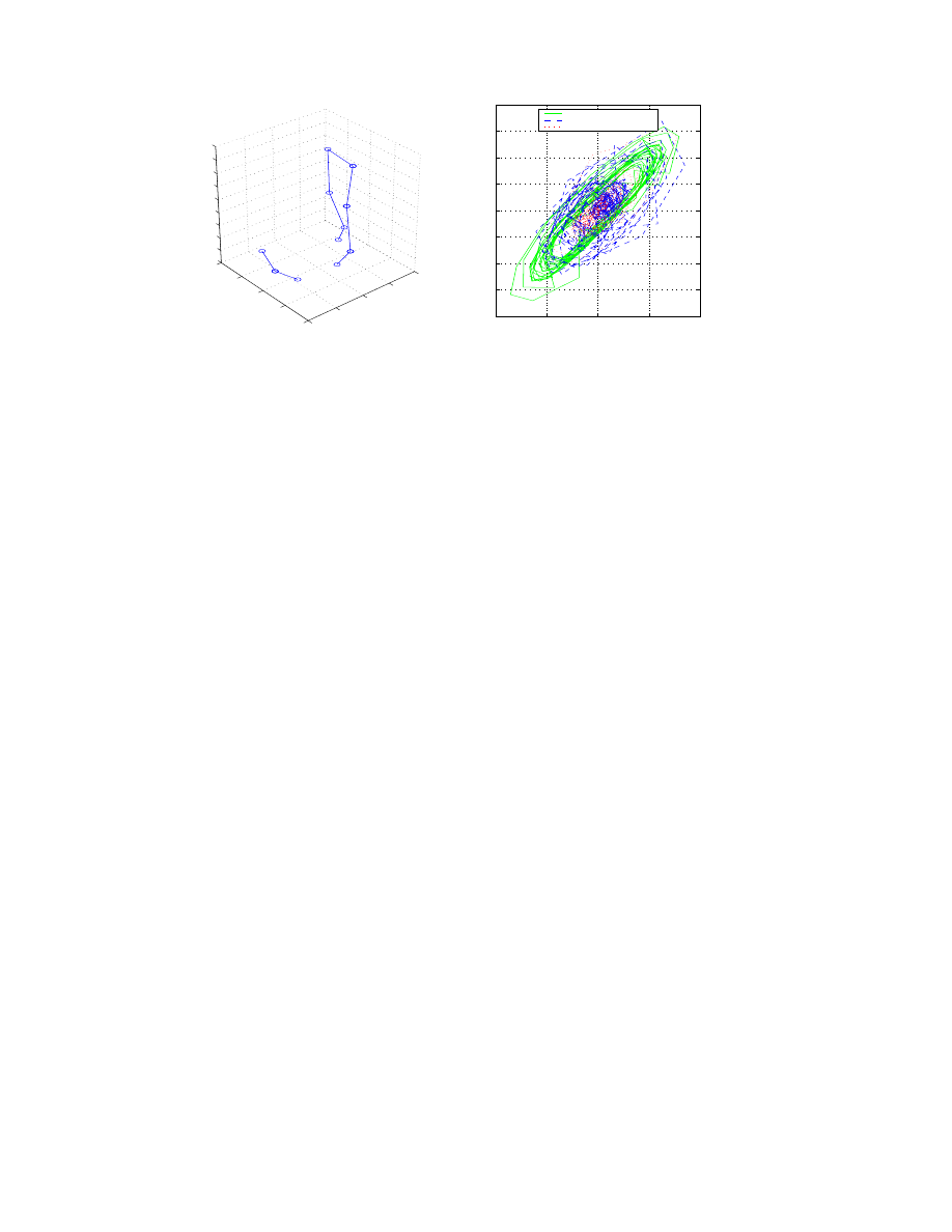
Real world applications and results

The above techniques were applied to a dataset obtained from a bridge simulator [20]. In this
case the bridge was oscillating with one degree of freedom and the human subject walking on
a treadmill on the bridge phase locked into the bridge oscillation. We have assumed that the
oscillation direction is horizontal even though in the actual simulator it has a vertical component.
Eight markers were placed on the joints of the legs of the human subject and three markers were

17

−4

−2

0

2

4

x 10

−3

−4

−3

−2

−1

0

1

2

3

4

x 10

−3

F

k

(foot)

F

k+1

(foot)

(b) Phase plot − delay one

measured force
force on right foot
force on left foot

0.6

0.8

1

1.2

1.4

−0.2

−0.1

0

0.1

0.2

−0.2

−0.15

−0.1

−0.05

0

0.05

0.1

0.15

0.2

0.25

x

5

5

7

7

6

6

3

3

4

8

2

2

1

1

(a) A frame of the motion capture dataset

11

10

10

9

y

z

Figure 5: (a) A frame of the motion capture data showing the legs of the subject and the
bridge markers. (b) The phase plot of the mechanically measured force on the bridge and
the forces calculated from the motion capture data.

placed on the bridge as shown in figure (5(a)). The markers were captured using a motion capture
system described in [21]. The output of the system is a set of 3D marker positions. Since in this
particular dataset a single marker per limb is placed at the joints, calculation of the joint location
and the rotation from one frame to the next was trivial. As this is not accurate, only qualitatively
accurate results were expected in this experiment. The limbs were modelled as solid cylinders with
axes assumed parallel to the vector between two joint markers. The principal axes and the inertia
tensors were calculated accordingly. The rotation from principal axes to the first frame (

r

r

(l

)

) was

calculated using the GA method given in [22]. The rotational bivectors were calculated from the
rotors representing the rotations from the principal axes to each frame. The calculated bivectors
were smoothed using Savitzky-Golay filters as implemented in [18] since the data is noisy and first
and second derivatives of the bivectors wrt time must be evaluated. The procedure described in
section (3.2) was then applied to the resulting data.

t

k

+1

(l

)

and

c

k

(l

)

were trivially calculated in

this case as the joint marker location and the half-way point on the corresponding link, respectively.

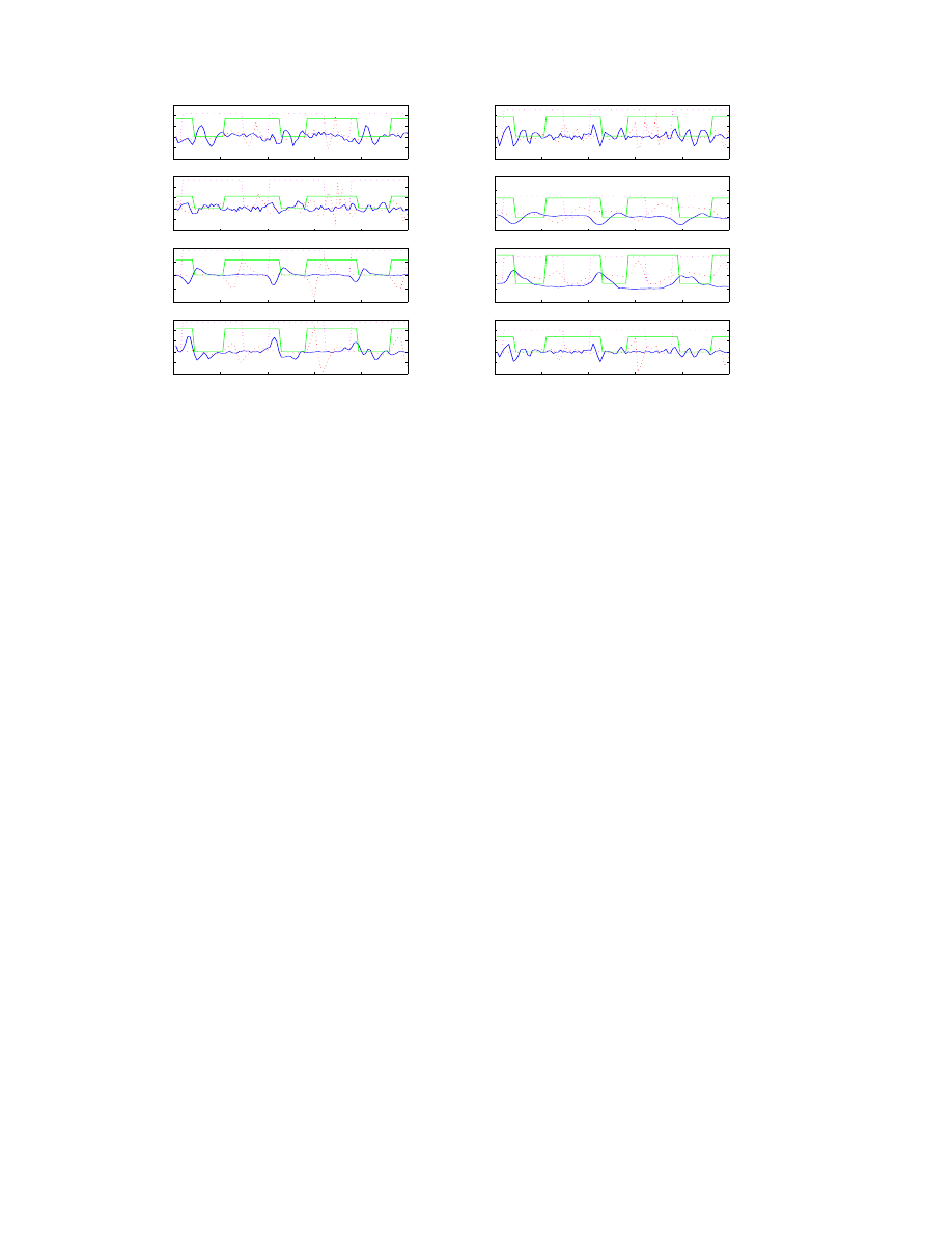
An example of the results are shown in figure (6) – many more plots are given in [16]. Also the
actual displacement of the bridge was measured mechanically. This displacement data was used
to calculate the bridge acceleration. The phase relationship of the acceleration of the bridge versus
that of the foot is compared in figure (5(b)).

These figures are presented as an illustration of an application of the procedure described in this
paper. For example, note also that data from figure (6) suggests that the very marked twist of the
foot towards the end of the gait cycle (before the foot is raised) seems to be responsible for most
of the lateral force on the bridge from the walker. It is also clear that scalar quantities such as
the angular velocity of the foot (and indeed the lower leg and the upper leg although this data is
not shown here) make smooth cyclic patterns in all directions. Further work will compare the gait
patterns between walkers on swinging and stationary structures. These techniques can be used
to complement data from force plate measurements and can also be used directly for biomedical
engineering applications.

18

0

20

40

60

80

100

−4

−2

0

2

4

6

x 10

−3

(a) acceleration of the foot in oscillating direction

0

20

40

60

80

100

−2

−1

0

1

2

3

x 10

−3

(b) acc. due to rot. only of the foot in oscillating direction

0

20

40

60

80

100

−1

−0.5

0

0.5

1

1.5

x 10

−4

(c) d(ang. momentum)/dt of the foot in oscillating direction

0

20

40

60

80

100

−0.8

−0.6

−0.4

−0.2

0

(d) rotational bivector direction of the foot in oscillating direction

0

20

40

60

80

100

−0.1

−0.05

0

0.05

0.1

(e) d(rotational bivector direction)/dt of the foot in oscillating direction

0

20

40

60

80

100

1.4

1.6

1.8

2

2.2

(f) rotational angle of the foot

radians

0

20

40

60

80

100

−0.1

−0.05

0

0.05

0.1

0.15

(g) angular velocity of the foot

0

20

40

60

80

100

−0.1

−0.05

0

0.05

0.1

0.15

(h) angular acceleration of the foot

Figure 6: (a)-(e) Inverse dynamics quantities of the foot in the approximate oscillating
direction of the bridge plane. (f)-(h) the absolute angle of rotation from the principal axis
to the current position, angular velocity and angular acceleration of the foot. The dotted
lines are left limb and the solid lines are right limb data in all figures. The rectangular
pulses represent the times the corresponding leg is in contact with the bridge. Note that
the y-axis is accurate only up to a scale factor unless labelled.

4.1

Conclusions and future work

Here we have described an algorithm to estimate the quantities relevant in inverse dynamics from
the 3D positions of the points on moving articulated bodies. Although we have mainly concen-
trated on data obtained visually, the techniques can be readily applied to other technologies, such
as magnetic markers. Most of the methods given here can also be used in robotics. In the applica-
tion dataset given, the joint locations and the rotations were estimated trivially. But in general, if
there are multiple markers per link, these quantities can be calculated in a least squares sense using
the techniques described in [23] and [19]. The crucial reason for the resulting simple recipe for
calculating inverse dynamic quantities is the use of a single GA quantity, the rotational bivector,
as the variable quantity rather than treating direction and magnitudes separately.

Clearly more experimental work is necessary to validate the procedures described here. Ideally
the algorithm should be cast in a probabilistic framework and also, a sensitivity analysis, similar
to that given in [10], should be carried out. Such an analysis would estimate the sensitivity of our
derived quantities to errors in the locations of points, models used etc.

We believe that, despite current limitations, the methods we have described here provide a set of
powerful tools for estimation of dynamical quantities for use in engineering, biomedical applica-
tions and computer animation.

19

References

[1] D. Hestenes and G. Sobczyk, Clifford Algebra to Geometric Calculus: A Unified Language

for Mathematics and Physics. D. Reidel: Dordrecht, 1984.

[2] D. Hestenes, New Foundations for Classical Mechanics.

Kluwer Academic Publishers,

2nd edition., 1999.

[3] C. Doran and A. Lasenby, “Physical applications of geometric algebra,”

Available at

http://www.mrao.cam.ac.uk/ clifford/ptIIIcourse/

. 1999.

[4] J. Lasenby, W. Fitzgerald, A. Lasenby, and C. Doran, “New geometric methods for com-

puter vision: An application to structure and motion estimation,” International Journal of
Computer Vision, vol. 26, no. 3, pp. 191–213, 1998.

[5] L.

Dorst,

S.

Mann,

and

T.

Bouma,

“GABLE:

A

MAT-

LAB

tutorial

for

geometric

algebra,”

Available

at

http://www.carol.wins.uva,nl/ leo/clifford/gablebeta.html

.2000.

[6] H. Goldstein, “Classical Mechanics,” Second Edition. Addison Wesley. 1980.

[7] J.M McCarthy, “An Introduction to Theoretical Kinematics”. MIT Press, Cambridge, MA.

1990.

[8] H. Li, D. Hestenes, A. Rockwood. “ Generalized Homogeneous Coordinates for Com-

putational Geometry”. G. Sommer, editor, Geometric Computing with Clifford Algebras.
Springer. To appear Summer 2001.

[9] D. Hestenes, D. “Old wine in new bottles: a new algebraic framework for computational

geometry”. Advances in Geometric Algebra with Applications in Science and Engineering,
Eds. Bayro-Corrochano, E.D. and Sobcyzk, G. Birkhauser Boston. To appear Summer 2000.

[10] B. Karan and M. Vukobratovi´c, “Calibration and accuracy of manipulation robot models -

an overview,” Mechanism and Machine Theory, vol. 29, no. 3, pp. 479–500, 1994.

[11] H. Asada and J. J. E. Slotine, Robot Analysis and Control. John Wiley and Sons, 1986.

[12] J. Luh, W. M.W., and P. R.P.C, “On-line computational scheme for mechanical manipula-

tors,” A.S.M.E. J. Dyn. Syst. Meas. Contr., no. 102, 1980.

[13] J. Apkarian, S. Naumann, and B. Cairns, “A three-dimentional kinematic and dynamic model

of the lower limb,” Journal of Biomechanics, vol. 22, no. 2, pp. 143–155, 1989.

[14] C. Doran and A. Lasenby, “Physical applications of geometric algebra,” 2001. Available at

http://www.mrao.cam.ac.uk/˜clifford/ptIIIcourse/

.

[15] D. Hestenes, New Foundations for Classical Mechanics. Kluwer Academic Publishers, sec-

ond ed., 1999.

[16] S. S. Hiniduma Udugama Gamage and J. Lasenby, “Extraction of rigid body dynamics from

motion capture data,” CUED Technical Report CUED/F-INFENG/TR.410, Cambridge Uni-
versity Engineering Department, 2001.

20

[17] F. A. McRobie and J. Lasenby, “Simo-Vu Quoc rods using Clifford algebra,” International

Journal for Numerical Methods in Engineering, vol. 45, pp. 377–398, 1999.

[18] W. H. Press, S. A. Teukolsky, W. T. Vetterling, and B. P. Flannery, Numerical Recipes in C.

Cambridge University Press, second ed., 1992.

[19] S. S. Hiniduma Udugama Gamage, M. Ringer, and J. Lasenby, “Estimation of centres and

axes of rotation of articulated bodies in general motion for global skeleton fitting,” CUED
Technical Report CUED/F-INFENG/TR.408, Cambridge University Engineering Depart-
ment, 2001.

[20] A. McRobie, G. Morgenthal, J. Lasenby, M. Ringer, and S. Gamage, “Millennium bridge

simulator.” Available at http://www2.eng.cam.ac.uk/˜gm249/MillenniumBridge/.

[21] M. Ringer and J. Lasenby, “Modelling and tracking articulated motion from muliple cam-

era views,” in Analysis of Biomedical Signals and Images: 15-th Biennial International
EURASIP conference Euroconference Biosignal 2000 Proceedings (J. Jan, J. Kozumpl´ik,
I. Provazn´ik, and Z. Szab´o, eds.), pp. 92–94, Brno University of Technology Vutium Press,
2000.

[22] J. Lasenby, W. Fitzgerald, A. Lasenby, and C. Doran, “New geometric methods for com-

puter vision: An application to structure and motion estimation,” International Journal of
Computer Vision, vol. 26, no. 3, pp. 191–213, 1998.

[23] S. S. Hiniduma Udugama Gamage and J. Lasenby, “A new least squares solution for esti-

mation of centre and axis of rotation,” CUED Technical Report CUED/F-INFENG/TR.399,
Cambridge University Engineering Department, 2001.

21