
4
Transport Properties in the Drying
of Solids
Dimitris Marinos-Kouris and Z.B. Maroulis
CONTENTS
ß
2006 by Taylor & Francis Group, LLC.

Acknowledgment ............................................................................................................................................ 112
Nomenclature ................................................................................................................................................. 112
References ...................................................................................................................................................... 114
4.1 INTRODUCTION
Drying is a complicated process involving simultan-
eous heat, mass, and momentum transfer phenomena,
and effective models are necessary for process design,
optimization, energy integration, and control. The
development of mathematical models to describe dry-
ing processes has been a topic of many research stud-
ies for several decades. Undoubtedly, the observed
progress has limited empiricism to a large extent.
However, the design of dryers is still a mixture of
science and practical experience. Thus the prediction
of Luikov that by 1985 ‘‘would obviate the need for
empiricism in selecting optimum drying conditions,’’
represented an optimistic perspective, which, how-
ever, shows that the efforts must be increased [1].
Presently, more and more sophisticated drying
models are becoming available, but a major question
that still remains is the measurement or determi-
nation of the parameters used in the models. The
measurement or estimation of the necessary param-
eters should be feasible and practical for general
applicability of a drying model.
In the early 1970s, Nonhebel and Moss stated that
‘‘the choice of drying plant, or design of special plant
to meet unprecedented conditions’’ would require use
of 34 parameters [2]. Regardless of the truth of such a
statement, that is, of the actual number of parameters
necessary for the design of a dryer, there is an obvious
need for a large amount of data. Nowadays, the
completeness and accuracy of such data reflect to a
large extent our ability to perform effective process
design. It should be noted that in spite of the intense
activities in the drying literature (Drying Technology
Journal, Advances in Drying, Drying, International
Drying Symposium, etc.), the problem of property
data still remains an important one because such
data are widely scattered and not systematically
evaluated. Moreover, whereas the need ‘‘for accurate
design data is increasing, the rate of accumulation
of new data is not increasing fast enough’’ [3]. The
lack of data is expected to continue and, as noted
by Keey, ‘‘it is probably unrealistic to expect com-
plete hygrothermal data for materials of commercial
interest’’ [4].
Out of the full set of thermophysical properties
necessary for the analysis of drying of a material, this
chapter examines only those that are critical. As such,
we consider the thermodynamic and transport prop-
erties, which are usually incorporated in a drying
model as model parameters, and which are:
Effective moisture diffusivity
Effective thermal conductivity
Air boundary heat and mass transfer coefficients
Drying constant
Equilibrium material moisture content
Effective thermal conductivity and effective mois-
ture diffusivity are related to internal heat and mass
transfer, respectively, while air boundary heat and
mass transfer coefficients are related to external heat
ß
2006 by Taylor & Francis Group, LLC.

and mass transfer, respectively. The above transport
properties are usually coefficients in the correspond-
ing flow rate and driving force relationship. The equi-
librium material moisture content, on the other hand,
is usually related to the mass transfer driving force.
The above transport properties in conjunction
with a transport phenomena mechanistic model can
adequately describe the drying kinetics, but some-
times an additional property, the drying constant, is
also used. The drying constant is essentially a com-
bination of the above transport properties and it must
be used in conjunction with the so-called thin-layer
model.
Effective moisture diffusivity and effective ther-
mal conductivity are in general functions of material
moisture content and temperature, as well as of the
material structure. Air boundary coefficients are func-
tions of the conditions of the drying air, that is hu-
midity, temperature, and velocity, as well as system
geometry. Equilibrium moisture content of a given
material is a function of air humidity and tempera-
ture. The drying constant is a function of material
moisture content, temperature, and thickness, as well
as air humidity, temperature, and velocity.
The required accuracy of the above properties
depends on the controlling resistance to heat and
mass transfer. If, for example, drying is controlled
by the internal moisture diffusion, then the effective
moisture diffusivity must be known with high accur-
acy. This situation is valid when large particles are
drying with air of high velocity. Drying of small
particles with low velocity of air is controlled by the
external mass transfer, and the corresponding coeffi-
cient should be known with high accuracy. But there
are situations in which heat transfer is the controlling
resistance. This happens, for example, in drying of
solids with high porosity, in which high mass and
low heat transfer rates are obtained.
The purpose of this chapter is to examine the
above properties related to drying processes, particu-
larly drying kinetics. Most of the following topics are
discussed for each property:
Definition
Methods of experimental measurement
Data compilation
Effect of various factors
Theoretical estimation
The statement of Poersch (quoted in Ref. [4]) that
it is possible for someone to dry a product based on
experience and without theoretical knowledge but not
the reverse is worth repeating here. To this we may
add the comment that it is impossible to efficiently
dry a product without complete and precise thermo-
physical data.
4.2 MOISTURE DIFFUSIVITY
4.2.1 D
EFINITION
Diffusion in solids during drying is a complex process
that may involve molecular diffusion, capillary flow,
Knudsen flow, hydrodynamic flow, or surface diffusion.
If we combine all these phenomena into one, the effect-
ive diffusivity can be defined from Fick’s second law
@X =@t
¼ D r
2
X (4 :1)
where D (m
2
/s) is the effective diffusivity, X (kg/kg
db) is the material moisture content, and t (s) is the
time.
The moisture transfer in heterogeneous media can
be conveniently analyzed by using Fick’s law for
homogeneous materials, in which the heterogeneity
of the material is accounted for by the use of an
effective diffusivity.
Equation 4.1 shows the time change of the mater-
ial moisture distribution, that is, it describes the
movement of moisture within the solid. The previous
equation can be used for design purposes in cases in
which the controlling mechanism of drying is the
diffusion of moisture.
Pakowski and Mujumdar [5] describe the use of
Equation 4.1 for the calculation of the drying rate,
whereas Strumillo and Kudra [6] describe its use in
calculating the drying time. Solutions of the Fickian
equation for a variety of initial and boundary condi-
tions are exhaustively described by Crank [7].
4.2.2 M
ETHODS OF
E
XPERIMENTAL
M
EASUREMENT
There is no standard method for the experimental
determination of diffusivity. The diffusivity in solids
can be determined using the methods presented in
. These methods have been developed pri-
marily for polymeric materials [7–9]. Table 4.1 also
includes the relevant entries in the ‘‘References’’ sec-
tion for the application of the methods in food systems.
4.2.2.1 Sorption Kinetics
The sorption (adsorption or desorption) rate is meas-
ured with a sorption balance (spring or electrical)
whereas the solid sample is kept in a controlled envir-
onment. Assuming negligible surface resistance to
mass transfer, the method is based on Fick’s diffusion
equation.
ß
2006 by Taylor & Francis Group, LLC.

4.2.2.2 Permeation Method
The permeation method is a steady-state method ap-
plied to a film of material. According to this method,
the permeation rate of a diffusant through a material
of known thickness is measured under constant, well-
defined, surface concentrations. The analysis is also
based on Fick’s diffusion equation.
4.2.2.3 Concentration–Distance Curves
The concentration–distance curves method is based
on the measurement of the distribution of the diffu-
sant concentration as a function of time. Light inter-
ference methods, as well as radiation adsorption or
simply gravimetric methods, can be used for concen-
tration measurements. Various sample geometries can
be used, for example semiinfinite solid, two joint cy-
linders with the same or different material, and so
on. The analysis is based on the solution of Fick’s
equation.
4.2.2.4 Other Methods
Modern methods for the measurement of moisture
profiles lead to diffusivity measurement methods.
Such methods discussed in the literature are radio-
tracer methods, nuclear magnetic resonance (NMR),
electron spin resonance (ESR), and the like.
4.2.2.5 Drying Methods
The simplified, regular regime, and regression analy-
sis methods are particularly relevant for drying
processes. In them, the samples are placed in a dryer
and moisture diffusivity is estimated from drying
data. All the drying methods are based on Fick’s
equation of diffusion, and they differ with respect to
the solution methodology. The following analysis is
considered.
4.2.2.5.1 Simplified Methods
Fick’s equation is solved analytically for certain sam-
ple geometries under the following assumptions:
Surface mass transfer coefficient is high enough so
that the material moisture content at the surface
is in equilibrium with the air drying conditions.
Air drying conditions are constant.
Moisture diffusivity is constant, independent of
material moisture content and temperature.
The analytical solution for slab, spherical, or
cylindrical samples is used in the analysis. Several
alternatives exist concerning the methodology of esti-
mation of diffusivity using the above equations. They
are discussed in the COST 90bis project of European
Economic Community (EEC) [16]. These alternatives
differ essentially on the variable on which a regression
analysis is applied.
4.2.2.5.2 Regular Regime Method
The regular regime method is based on the experi-
mental measurement of the regular regime curve,
which is the drying curve when it becomes independ-
ent of the initial concentration profile. Using this
method, the concentration-dependent diffusivity can
be calculated from one experiment.
4.2.2.5.3 Numerical Solution—Regression Analysis
Method
The regression analysis method can be considered as
a generalization of the other two types of methods.
It can estimate simultaneously some additional
transport properties; it is analyzed in detail in
.
4.2.3 D
ATA
C
OMPILATION
Effective diffusivities, reported in the literature, have
been usually estimated from drying or sorption rate
data. Experimental data are scarce because of the
effect of the experimental method, the method of
analysis, the variations in composition and structure
of the examined materials, and so on. Data of effect-
ive diffusion coefficients are available for inorganic
materials [20], polymers [8], and foods [21,22].
gives some literature values of the
effective diffusivity of moisture in various materials.
A number of data from the above-mentioned biblio-
graphic entries are also included in Table 4.2. New
data up to 1992 are also incorporated. Foods are the
TABLE 4.1
Methods for the Experimental Measurement
of Moisture Diffusivity
Method
Ref.
Sorption kinetics
8
Permeation methods
8
Concentration–distance curves
10–12
Other methods
Radiotracer methods
8
Nuclear magnetic resonance (NMR)
8, 13, 14
Electron spin resonance (ESR)
8, 15
Drying technique
Simplified methods
16
Regular regime method
17–19
Numerical solution—regression analysis
See Section 4.7
ß
2006 by Taylor & Francis Group, LLC.

TABLE 4.2
Effective Moisture Diffusivity in Some Materials
Classification
a
Material
Water Content (kg/kg db)
Temperature (8C)
Diffusivity (m
2
/s)
Ref.
Food
1
Alfalfa stems
<
3.70
26
2.6E-12–2.6E-09
23
2
Apple
0.12
60
6.5E-12–1.2E-10
24
0.15–7.00
30–76
1.2E-10–2.6E-10
25
3
Avocado
31–56
1.1E-10–3.3E-10
26
4
Beet
65
1.5E-09
26
5
Biscuit
0.10–0.65
20–100
9.4E-10–9.7E-08
27
6
Bread
0.10–0.70
20–100
2.5E-09–5.5E-07
27
7
Carrot
0.03–11.6
42–80
9.0E-10–3.3E-09
28
8
Corn
0.05–0.23
40
1.0E-12–1.0E-10
29
0.19–0.27
36–62
7.2E-11–3.3E-10
30
9
Fish muscle
0.05–0.30
30
8.1E-11–3.4E-10
31
10
Garlic
0.20–1.60
22–58
1.1E-11–2.0E-10
32
11
Milk foam
0.20
40
1.1E-09
33
Milk skim
0.25–0.80
30–70
1.5E-11–2.5E-10
34
12
Muffin
0.10–0.65
20–100
8.4E-10–1.5E-07
27
13
Onion
0.05–18.7
47–81
7.0E-10–4.9E-09
35
14
Pasta, semolina
0.01–0.25
40–125
3.0E-13–1.5E-10
36
Pasta, corn based
0.10–0.40
40–80
5.0E-11–1.3E-10
37
Pasta, durum wheat
0.16–0.35
50–90
2.5E-12–5.6E-11
38
15
Pepper, green
0.04–16.2
47–81
5.0E-10–9.2E-09
35
16
Pepperoni
0.19
12
4.7E-11–5.7E-11
39
17
Potato
0.60
54
2.6E-10
40
<
4.00
65
4.0E-10
41
0.15–3.50
65
1.7E-09
42
0.01–7.20
39–82
5.0E-11–2.7E-09
43
18
Rice
0.18–0.36
60
1.3E-11–2.3E-11
44
0.28–0.64
40–56
1.0E-11–6.9E-11
45
19
Soybeans, defatted
0.05
30
2.0E-12–5.4E-12
46
20
Starch, gel
0.10–0.30
25
1.0E-12–2.3E-11
47
0.20–3.00
30–50
1.0E-10–1.2E-09
48
0.75
25–140
1.0E-10–1.5E-09
49
Starch granular
0.10–0.50
25–140
5.0E-10–3.0E-09
49
21
Sugar beet
2.50–3.60
40–80
4.0E-10–1.3E-09
50, 51
22
Tapioca root
0.16–1.95
97
9.0E-10
52, 53
23
Turkey
0.04
22
8.0E-15
54
24
Wheat
0.12–0.30
21–80
6.9E-12–2.8E-10
55
0.13–0.20
20
3.3E-10–3.7E-09
56
Other materials
1
Asbestos cement
0.10–0.60
20
2.0E-09–5.0E-09
20
2
Avicel (FMC Corp.)
37
5.0E-09–5.0E-08
57
3
Brick powder
0.08–0.16
60
2.5E-08–2.5E-06
58
4
Carbon, activated
25
1.6E-05
59
5
Cellulose acetate
0.05–0.12
25
2.0E-12–3.2E-12
60
6
Clay brick
0.20
25
1.3E-08–1.4E-08
61
7
Concrete
0.10–0.40
20
5.0E-10–1.2E-08
20
Concrete, pumice
0.20
25
1.8E-08
61
8
Diatomite
0.05–0.50
20
3.0E-09–5.0E-09
20
9
Glass wool
0.10–1.80
20
2.0E-09–1.5E-08
20
Glass spheres, 10 mm
0.01–0.22
60
1.84E-8 + 0.94E-8
16
10
Hyde clay
0.10–0.40
5.0E-09–1.0E-08
62
11
Kaolin clay
<
0.50
45
1.5E-08–1.5E-07
20
12
Model system
68
3.1E-09
63
continued
ß
2006 by Taylor & Francis Group, LLC.

most investigated materials in the literature, and they
are presented separately. Table 4.2 was prepared for
the needs of this chapter, that is, to show the range of
variation of diffusivity for various materials and not
to present some experimental values. That is why
most of the data are presented as ranges.
The data of Table 4.2 are further displayed in
through Figure 4.4. The moisture diffusiv-
ity is plotted versus the number of material for food
and other materials in Figure 4.1. Diffusivities in
foods have values in the range 10
13
to 10
6
m
2
/s,
and most of them (82%) are accumulated in the re-
gion 10
11
to 10
8
. Diffusivities of other materials
have values in the range 10
12
to 10
5
, whereas
most of them (58%) are accumulated in the region
10
9
to 10
7
. These results are also clarified in the
. Diffusivities in foods are
less than those in other materials. This is because of
the complicated biopolymer structure of food and,
probably, the stronger binding of water in them.
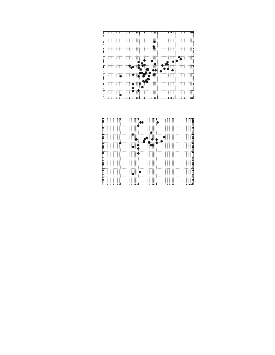
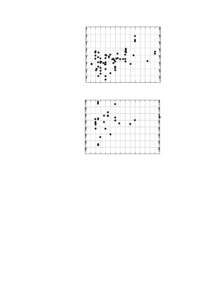
The influence of material moisture content and
temperature from the statistical point of view is
shown in Figure 4.3 and Figure 4.4. Figure 4.3
shows the diffusivities versus the material moisture
content for all the materials. The positive effect of
material moisture content on diffusivity is evident.
The same trend is noted in Figure 4.4 with regard to
the temperature. It should be noted that the observed
trends in the previous figures are the result of exam-
ining different materials at various temperatures and
moistures and from various sources. The influence of
material moisture content and temperature for each
material is discussed in the next section.
In general, comparison among diffusivities
reported in the literature is difficult because of the
different methods of estimation and the variation of
composition, especially for foods. However, on the
, it is concluded that
the differences in diffusivity among materials are less
than that between temperature or material moisture
content of the same material. Diffusivities of other
solutes in various materials are also presented in the
literature (e.g., see Ref. [68]).
4.2.4 F
ACTORS
A
FFECTING
D
IFFUSIVITY
Moisture diffusivity depends strongly on temperature
and, often, very strongly on the moisture content, but
there are few reliable figures. In porous materials the
void fraction affects diffusivity significantly, and the
pore structure and distribution do so even more.
The temperature dependence of the diffusivity can
generally be described by the Arrhenius equation,
which takes the form
D
¼ D
O
exp (
E=RT)
(4:2)
where D
O
(m
2
/s) is the Arrhenius factor, E (kJ/kmol)
is the activation energy for diffusion, R (kJ/(kmol K))
the gas constant, and T (K) the temperature.
The moisture content dependence of the diffusiv-
ity can be introduced in the Arrhenius equation by
considering either the activation energy or the Arrhe-
nius factor as an empirical function of moisture. Both
modifications can be considered simultaneously.
Other empirical equations not based on the Arrhenius
equation can be used.
The moisture diffusivity is an increasing function
of the temperature and moisture of the material. Yet,
in certain categories of polymers, deviation from this
kind of behavior has been observed. For instance, for
several of the less hydrophilic polymers (e.g., poly-
methacrylates and polycrylates) the moisture diffusiv-
ity decreases with increasing water content. On the
TABLE 4.2 (contin ued)
Effective Moisture Diffusi vity in Some Materia ls
Classification
a
Material
Water Content (kg/kg db)
Temperature ( 8C)
Diffusivity (m
2
/s)
Ref.
13 Peat
0.30–2.50 45 4.0E-08–5.0E-08 20
14 Sand <0.15 45 8.0E-08–1.5E-07
20
Sand, sea 0.07–0.13
60 2.5E-08–2.5E-06 58
Sand
0.05–0.10 1.0E-07–1.0E-06 64
15
Silica alumina 0.59–1.18
60 2.5E-08–2.5E-06 58
16
Silica gel
25
3.0E-06–5.6E-06
59
17
Tobacco leaf
30–50
3.2E-11–8.1E-11
65
18
Wood, soft
40–90
5.0E-10–2.5E-09
66
Wood, yellow poplar
1.00
100–150
1.0E-08–2.5E-08
67
a
Classification number for each material used in Figure 4.1.
ß
2006 by Taylor & Francis Group, LLC.

other hand, the moisture diffusivity appears to be
independent of the concentration—and hence con-
stant—for some hydrophobic polyolefins.
gives some relationships that describe
simultaneous dependence of the diffusivity upon tem-
perature and moisture. Some rearrangement of the
equations proposed has been done in order to present
them in a uniform format.
values for typical equations of Table 4.3.
Equation T3.1 through Equation T3.4 in Table
4.3 suggest that the material moisture content can be
taken into account by considering the preexponential
factor of the Arrhenius equation as a function of
material moisture content. Polynomial functions of
first order can be considered (Equation T3.1), as
well as of higher order (Equation T3.2 or Equation
T3.3). The exponential function can also be used
(Equation T3.4).
Equation T3.5 and Equation T3.6 in Table 4.3 are
obtained by considering the activation energy for
diffusion as a function of material moisture content.
Equation T3.7 through Equation T3.10 are not based
on the Arrhenius form. They are empirical and they use
complicated functions concerning the discrimination
of the moisture and temperature effects (except, of
course, Equation T3.7). Equation T3.11 is more so-
phisticated as it considers different diffusivities of
bound and free water and introduces the functional
dependence of material moisture content on the bind-
ing energy of desorption. Equation T3.12 introduces
the effect of porosity on moisture diffusivity.
With regard to the number of parameters involved
(a significant measure concerning the regression an-
alysis), it is concluded that at least three parameters
are needed (Equation T3.1, Equation T3.5, and Equa-
tion T3.7).
Equation T3.5 and Equation T3.7 in Table 4.3
were applied to potato and clay brick, respectively,
and the results are presented in
. Both
materials exhibit typical behavior. Diffusivity at low
0
10
−13
10
−11
10
−9
10
−7
10
−5
5
10
15
20
25
Moisture
diffusivity
(m
2
/s)
Number of material on Table 4.2
0
Other materials
10
−13
10
−11
10
−9
10
−7
10
−5
5
10
15
25
Moisture
diffusivity
(m
2
/s)
Number of material on Table 4.2
Food materials
FIGURE 4.1 Moisture diffusivity in various materials (data from
).
ß
2006 by Taylor & Francis Group, LLC.
moisture content shows a steep descent when the moi-
sture content decreases.
resulted from
fitting to experimental data. The reason for the success
of this procedure is the apparent simple dependence of
diffusivity upon the material moisture content and
temperature, which, as stated above, can be described
even by three parameters only. The equations of Table
4.3 have been chosen by the respective researchers as
the most appropriate for the material listed.
A single relation for the dependence of diffusivity
upon the material moisture content and temperature
general enough so as to apply to all the materials
would be especially useful. It is expected that such a
relation will be proposed soon.
The effect of pore structure and distribution on
moisture diffusion can be examined by considering
the material as a two-(or multi-) phase (dry material,
water, air in voids, etc.) system and by considering
some structural models to express the system geom-
etry. Although a lot of work has been done in
the analogous case of thermal conductivity, little
attention has been given to the case of moisture dif-
fusivity, and even less experimental validation of the
structural models has been obtained. The similarity,
however, of the relevant transport phenomena (i.e.,
heat and mass transfer) permits, under certain restric-
tions, the use of conclusions derived from one area in
the other. Thus, the literature correlations for the
estimation of the effective diffusion coefficient, in
many cases, had been initially developed for the ther-
mal conductivity in porous media [79].
4.2.5 T
HEORETICAL
E
STIMATION
The prediction of the diffusion coefficients of gases
from basic thermophysical and molecular properties is
possible with great accuracy using the Chapman–Enskog
−13
0
5
10
20
25
15
−12
−11
−10
−9
−8
−7
−6
−5
Number
of values
accounted
log(
D)
−13
0
2
4
6
6
10
12
24
−12
−11
−10
−9
−8
−7
−6
−5
Number
of values
accounted
log(
D)
Food materials
Other materials
FIGURE 4.2 Histograms of diffusivities in various materials (data from
).
ß
2006 by Taylor & Francis Group, LLC.
kinetic theory. Diffusivities in liquids, on the other
hand, in spite of the absence of a rigorous theory, can
be estimated within an order of magnitude from the
well-known equations of Stokes and Einstein (for
large spherical molecules) and Wilke (for dilute solu-
tions).
Diffusion of gases, vapors, and liquids in solids,
however, is a more complex process than the diffusion
in fluids because of the heterogeneous structure of the
solid and its interactions with the diffusing compon-
ents. As a result, it has not yet been possible to
develop an effective theory for the diffusion in solids.
Usually, diffusion in solids is handled by the re-
searchers in a manner analogous to heat conduction.
In the following paragraphs typical methods are de-
scribed for the development of semiempirical correl-
ations for diffusivity.
For the estimation of the diffusion coefficient in
isotropic macroporous media, the relation
D
¼ ( d«=t
2
)D
A
(4 :3)
has been proposed [79]. In this equation, « is the
porosity, t is the tortuosity, d is the constrictivity,
and D
A
is the vapor diffusivity in air in the absence
of porous media. In spite of its simplicity, Equation
4.3 will not attain practical utility unless it is validated
with additional pore space models, its parameters ( «,
t
, d) determined for a large number of systems, and
the effect of the solid’s moisture properly accounted
for.
An equation has been derived relating the effective
diffusivity of porous foodstuffs to various physical
properties such as molecular weight, bulk density,
vapor space permeability, water activity as a function
of material moisture content, water vapor pressure,
thermal conductivity, heat of sorption, and tempera-
ture [80]. A predictive model has been proposed to
obtain effective diffusivities in cellular foods. The
10
−3
10
−13
10
−11
10
−9
10
−7
10
−5
10
−2
10
−1
10
0
10
1
10
2
Moisture
diffusivity
(m
2
/s)
10
−3
10
−13
10
−11
10
−9
10
−7
10
−5
10
−2
10
−1
10
0
10
1
10
2
Moisture
diffusivity
(m
2
/s)
Material moisture content (kg/kg db)
Material moisture content (kg/kg db)
Food materials
Other materials
FIGURE 4.3 Moisture diffusivity versus material moisture content (data from
).
ß
2006 by Taylor & Francis Group, LLC.
method requires data for composition, binary mo-
lecular diffusivities, densities, membrane and cell
wall permeabilities, molecular weights, and water vis-
cosity and molar volume [81]. The effect of moisture
upon the effective diffusivity is taken into account via
the binding energy of sorption in an equation sug-
gested in Ref. [77].
4.3 THERMAL CONDUCTIVITY
4.3.1 D
EFINITION
The thermal conductivity of a material is a measure of
its ability to conduct heat. It can be defined using
Fourier’s law for homogeneous materials:
@T =@t
¼ (k=c
p
)
r
2
T (4 :4)
where k is the thermal conductivity (kW/(m K)), r is
the density (kg/m
3
), c
p
is the specific heat of the
material (kJ/(kg K)), T is the temperature (K), and t
is the time (s). The quantity (k/@c
p
) is the thermal
diffusivity. For heterogeneous materials, the effective
thermal conductivity is used in conjunction with
Fourier’s law.
Equation 4.4 is used in cases in which heat trans-
fer during drying takes place through conduction
(internally controlled drying). This, for example, is the
situation when drying large particles, relatively immo-
bile, that are immersed in the heat transfer medium.
As far as heat and mass transfer is concerned, the
drying process is internally controlled whenever the
respective Biot number (Bi
H
, Bi
M
) is greater than 1 [5].
4.3.2 M
ETHODS OF
E
XPERIMENTAL
M
EASUREMENT
The effective thermal conductivity can be determined
using the methods presented in
, which in-
cludes the relevant references. Measurement tech-
niques for thermal conductivity can be grouped into
0
10
−13
10
−11
10
−9
10
−7
10
−5
50 100 150
Temperature (
°C)
Food materials
Other materials
Moisture
diffusivity
(m
2
/s)
0
10
−13
10
−11
10
−9
10
−7
10
−5
50 100 150
Temperature (
°C)
Moisture
diffusivity
(m
2
/s)
FIGURE 4.4 Moisture diffusivity versus material temperature (data from
ß
2006 by Taylor & Francis Group, LLC.

steady-state and transient-state methods. Transient
methods are more popular because they can be run
for as short as 10 s, during which time the mois-
ture migration and other property changes are kept
minimal.
4.3.2.1 Steady-State Methods
In steady-state methods, the temperature distribution
of the sample is measured at steady state, with the
sample placed between a heat source and a heat sink.
TABLE 4.3
Effect of Material Moisture Content and Temperature on Diffusivity
Equation No.
Materials of Application
Equation
No. of
Parameters
Ref.
T3.1
Apple, carrot, starch
D(X,T)
¼ a
0
exp(a
1
X) exp(
a
2
/T)
3
49, 69, 70
T3.2
Bread, biscuit, muffin
D(X,T )
¼ a
0
exp
P
3
i
¼1
a
i
X
1
exp (
a
2
=T
)
5
27
T3.3
Polyvinylalcohol
D(X,T )
¼ a
0
exp
P
10
i
¼1
a
i
X
1
exp (
a
2
=T
)
12
71
T3.4
Vegetables
D(X,T)
¼ a
0
exp(
a
1
/X) exp(
a
2
/T)
3
72
T3.5
Glucose, coffee extract,
skim milk, apple, potato,
animal feed
D(X,T)
¼ a
0
exp[
a
1
(1/T
1/a
2
)]
a
1
¼ a
10
þ a
11
exp(
a
12
X)
5
18
T3.6
Silica gel
D(X,T)
¼ a
0
exp(
a
1
/T) a
1
¼ a
10
þ a
11
X
3
73
T3.7
Clay brick, burned clay,
pumice concrete
D(X,T)
¼ a
0
X
a
1
T
a
2
3
61
T3.8
Corn
D(X,T)
¼ a
0
exp(a
1
X) exp(
a
2
/T) a
1
¼ a
11
T
þ a
10
4
30
T3.9
Rough rice
D(X,T)
¼ a
1
exp(a
2
X) a
1
¼ a
10
exp(a
11
T),
a
2
¼ a
20
exp(a
21
T
þ a
22
T
2
)
5
74, 75
T3.10
Wheat
D(X,T)
¼ a
0
þ a
1
X
þ a
2
X
2
a
0
¼ a
01
exp(a
02
T),
a
1
¼ a
11
exp(a
12
T), a
2
¼ a
21
exp(a
22
T)
6
76
T3.11
Semolina, extruded
D(X,T )
¼ a
0
exp (
a
2
=T
)
a
2
exp (
a
3
=T
)
1
þ a
2
exp (
a
3
=T
)
4
77
T3.12
Porous starch
D(X,T )
¼ (a
0
þ a
1
X
a
2
) exp(
a
3
/T) a
0
¼ F(«)
>
5
78
D, moisture diffusivity; X, material moisture content; T, temperature; a
i
, constants; «, porosity.
TABLE 4.4
Application Examples
Material
Equation
Constants
Ref.
Clay brick, burned clay
D
¼ D
0
(T/T
0
)
a
T
(X/X
0
)
aX
D
0
¼ 7.36 · 10
9
m
2
/s, T
0
¼ 273 K, a
T
¼ 9.5,
X
0
¼ 0.35 kg/kg db, a
X
¼ 0.5 for clay brick;
D
0
¼ 1.11 · 10
9
m
2
/s, T
0
¼ 273 K, a
T
¼ 6.5,
X
0
¼ 0.40 kg/kg db, a
X
¼ 0.5 for burned clay
61
Polyvinylalcohol
D
¼ D
0
exp[
E/R(1/T 1/T
0
)],
D
0
¼ Sa
i
X
i
T
0
¼ 298 K, E ¼ 3.05 · 10
4
J/mol,
R
¼ 8.314 J/(mol K), a
0
¼ 0.104015 · 10
2
,
a
1
¼ 0.363457 · 10
2
, a
2
¼ 0.469291 · 10
3
,
a
3
¼ 0.634869 · 10
4
, a
4
¼ 0.517559 · 10
5
,
a
5
¼ 0.250188 · 10
6
, a
6
¼ 0.747613 · 10
6
,
a
7
¼ 0.139929 · 10
7
, a
8
¼ 0.159715 · 10
7
,
a
9
¼ 0.101503 · 10
7
, a
10
¼ 0.274672 · 10
6
71
Potato, carrot
D
¼ D
0
exp(
X
0
/X) exp(
T
0
/T)
D
0
¼ 2.41 · 10
7
m
2
/s, X
0
¼ 7.62 · 10
2
kg/kg db,
T
0
¼ 1.49 · 10
þ3
8
C for potato; D
0
¼ 2.68 · 10
4
m
2
/s,
X
0
¼ 8.92 · 10
2
kg/kg db, T
0
¼ 3.68 · 10
þ3
8
C for carrot
72
Silica gel
D
¼ D
0
exp( (E
0
E
1
X)/T)
D
0
¼ 5.71 · 10
7
m
2
/s, E
0
¼ 2450 K, E
1
¼ 1400 K/(kg/kg db)
73
ß
2006 by Taylor & Francis Group, LLC.
Different geometries can be used, those for longitu-
dinal heat flow and radial heat flow.
4.3.2.2 Longitudinal Heat Flow (Guarded
Hot Plate)
The longitudinal heat flow (guarded hot plate)
method is regarded as the most accurate and most
widely used apparatus for the measurement of ther-
mal conductivity of poor conductors of heat. This
method is most suitable for dry homogeneous speci-
mens in slab forms. The details of the technique are
given by the American Society for Testing and
Materials (ASTM) Standard C-177 [82].
4.3.2.3 Radial Heat Flow
Whereas the longitudinal heat flow methods are most
suitable for slab specimens, the radial heat flow techni-
ques are used for loose, unconsolidated powder or granu-
lar materials. The methods can be classified as follows:
Cylinder with or without end guards
Sphere with central heating source
Concentric cylinder comparative method
4.3.2.4 Unsteady State Methods
Transient-state or unsteady-state methods make use
of either a line source of heat or plane sources of heat.
0
× 10
0
1
× 10
−9
2
× 10
−9
3
× 10
−9
4
× 10
−9
5
× 10
−9
10
−9
10
−8
10
−7
10
−6
0
0.4
0.8
1.2
1.6
Water content (kg/kg db)
0
0.2
0.4
0.6
Water content (kg/kg db)
Moisture
diffusivity
(m
2
/s)
Moisture
diffusivity
(m
2
/s)
Potato
Clay brick
100
°C
100
°C
20
°C
20
°C
60
°C
60
°C
FIGURE 4.5 Effect of material moisture content and temperature on moisture diffusivity. Data for potato are
from Kiranoudis, C.T., Maroulis, Z.B., and Marinos-Kouris, D., Drying Technol., 10(4), 1097, 1992 and data for clay
brick are from Haertling, M., in Drying ’80, Vol. 1, A.S. Mujumdar (Ed.), Hemisphere Publishing, New York, 1980,
pp. 88–98.
ß
2006 by Taylor & Francis Group, LLC.

In both cases, the usual procedure is to apply a steady
heat flux to the specimen, which must be initially in
thermal equilibrium, and to measure the temperature
rise at some point in the specimen, resulting from this
applied flux [83]. The Fitch method is one of the most
common transient methods for measuring the thermal
conductivity of poor conductors. This method was
developed in 1935 and was described in the National
Bureau of Standards Research Report No. 561.
Experimental apparatus is commercially available.
4.3.2.5 Pro be Metho d
The probe method is one of the most common tran-
sient methods using a line heat source. This method is
simple and quick. The probe is a needle of good
thermal conductivity that is provided with a heater
wire over its length and some means of measuring the
temperature at the center of its length. Having the
probe embedded in the sample, the temperature re-
sponse of the probe is measured in a step change of
heat source and the thermal conductivity is estimated
using the transient solution of Fourier’s law. Detailed
descriptions as well as the necessary modifications for
the application of the above-mentioned methods in
food systems are given in Refs. [83,89,90].
4.3.3 D
ATA
C
OMPILATION
Despite the limited data of effective moisture diffu-
sivity, a lot of data are reported in the literature for
thermal conductivity. Data for mainly homogeneous
materials are available in handbooks such as the
Handbook of Chemistry and Physics [91], the Chemical
Engineers’ Handbook [92], ASHRAE Handbook of
Fundamentals [93], Rohsenow and Choi [94], and
many others. For foods and agricultural products,
data are available in Refs. [83,88,95–97]. For selected
pharmaceutical materials, data are presented by
Pakowski and Mujumdar [98].
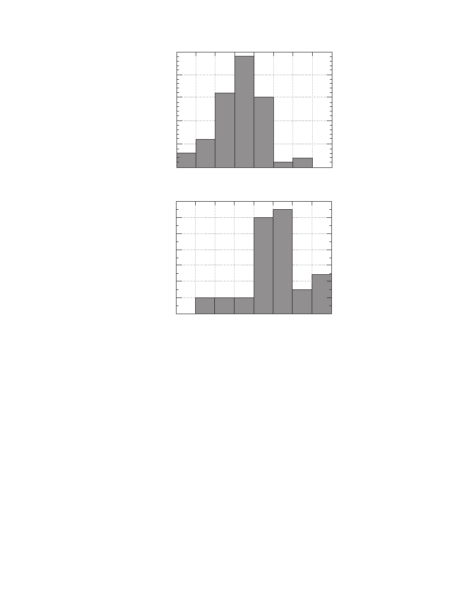
Some data for thermal conductivity are presented
in Table 4.6. These values are distributed as shown in
. The distribution is different from that of
moisture diffusivity (
), which is normal. For
thermal conductivity, the values are uniformly dis-
tributed in the range 0.25 to 2.25 W/(m K), whereas
a lot of data are accumulated below 0.25 W/(m K).
4.3.4 F
ACTORS
A
FFECTING
T
HERMAL
C
ONDUCTIVITY
The thermal conductivity of homogeneous materials
depends on temperature and composition, and empir-
ical equations are used for its estimation. For each
material, polynomial functions of first or higher order
TABLE 4.5
Methods for the Experimental Measurement
of Thermal Conductivity
Method
Ref.
Steady-state method
Longitudinal heat flow (guarded hot plate)
82
Radial heat flow
83
Unsteady-state method
Fitch
84, 85
Plane heat source
86
Probe method
87, 88
TABLE 4.6
Effective Thermal Conductivity in Some Materials
Material
Temperature
(8C)
Thermal
Conductivity
(W/(m K))
Ref.
Aerogel, silica
38
0.022
94
Asbestos
427
0.225
94
Bakelite
20
0.232
94
Beef, 69.5% water
18
0.622
99
Beef fat, 9% water
10
0.311
100
Brick, common
20
0.173–0.346
94
Brick, fire clay
800
1.37
94
Carrots
15 to 19
0.622
101
Concrete
20
0.813–1.40
94
Corkboard
38
0.043
94
Diatomaceous earth
38
0.052
94
Fiber-insulating board
38
0.042
94
Fish
20
1.50
100
Fish, cod, and haddock
20
1.83
102
Fish muscle
23
1.82
103
Glass, window
20
0.882
94
Glass wool, fine
38
0.054
94
Glass wool, packed
38
0.038
94
Ice
0
2.21
94
Magnesia
38
0.067
94
Marble
20
2.77
94
Paper
0.130
94
Peach
18–27
1.12
104
Peas
18–27
1.05
104
Peas
12 to 20
0.501
101
Plums
13 to 17
0.294
101
Potato
10 to 15
1.09
101
Potato flesh
18–27
1.05
104
Rock wool
38
0.040
94
Rubber, hard
0
0.150
94
Strawberries
18–27
1.35
104
Turkey breast
25
0.167
100
Turkey leg
25
1.51
100
Wood, oak
21
0.207
94
ß
2006 by Taylor & Francis Group, LLC.

are used to express the temperature effect. A large
number of empirical equations for the calculation of
thermal conductivity as a function of temperature
and humidity are available in the literature [83,92].
For heterogeneous materials, the effect of geom-
etry must be considered using structural models. Util-
izing Maxwell’s and Eucken’s work in the field of
electricity, Luikov et al. [105] initially used the idea
of an elementary cell, as representative of the model
structure of materials, to calculate the effective ther-
mal conductivity of powdered systems and solid por-
ous materials. In the same paper, a method is
proposed for the estimation of the effective thermal
conductivity of mixtures of powdered and solid
porous materials.
Since then, a number of structural models have
been proposed, some of which are given in Table 4.7.
The perpendicular model assumes that heat conduction
is perpendicular to alternate layers of the two phases,
whereas the parallel model assumes that the two
phases are parallel to heat conduction. In the mixed
model, heat conduction is assumed to take place by a
combination of parallel and perpendicular heat flow.
In the random model, the two phases are assumed
to be mixed randomly. The Maxwell model assumes
that one phase is continuous, whereas the other
phase is dispersed as uniform spheres. Several other
models have been reviewed in Refs. [107,110,111],
among others.
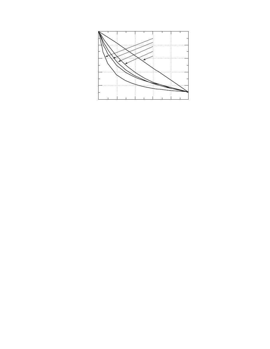
The use of some of these structural models to
calculate the thermal conductivity of a hypothetical
porous material is presented in
. The paral-
lel model gives the larger value for the effective ther-
mal conductivity, whereas the perpendicular model
gives the lower value. All other models predict values
in between. The use of structural models has been
0
0
0.5 1
2
4
6
8
10
12
14
16
2
Values of thermal conductivity (W/(m k))
Number
of values
accounted
3
1.5 2.5
FIGURE 4.6 Distribution of thermal conductivity values (data from
TABLE 4.7
Structural Models for Thermal Conductivity in Heterogeneous Materials
Model
Equation
Ref.
Perpendicular (series)
1/k
¼ (1 «)/k
1
þ «/k
2
106,107
Parallel
k
¼ (1 «)k
1
þ «k
2
106,107
Mixed
1=k
¼
1
F
(1
«)k
1
þ «k
2
þ F
1
«
k
1
þ
«
k
2
106,107
Random
k
¼ k
(1
e)
1
k
«
2
106,107
Effective medium theory
k
¼ k
1
[b
þ (b
2
þ 2(k
1
/k
2
)/(Z
2))
1/2
]
b
¼ [Z(1 «)/2 1 þ (k
2
/k
1
)(«Z/2
1)]/(Z 2)
108
Maxwell
k
¼
k
2
[k
1
þ 2k
2
2(1 «)(k
2
k
1
)]
k
1
þ 2k
2
þ (1 «)(k
2
k
1
)
109
k, Effective thermal conductivity; k
1
, thermal conductivities of phase i; «, void fraction of phase 2; F, Z, parameters.
ß
2006 by Taylor & Francis Group, LLC.
successfully extended to foods [108,112], which ex-
hibit a more complex structure than that of other
materials, whereas this structure often changes during
the heat conduction.
A systematic general procedure for selecting suit-
able structural models, even in multiphase systems,
has been proposed in Ref. [113]. This method is based
on a model discrimination procedure. If a component
has unknown thermal conductivity, the method esti-
mates the dependence of the temperature on the un-
known thermal conductivity, and the suitable structural
models simultaneously.
An excellent example of applicability of the above
is in the case of starch, a useful material in extrusion.
The granular starch consists of two phases, the wet
granules and the air–vapor mixture in the intergranu-
lar space. The starch granule also consists of two
phases, the dry starch and the water. Consequently,
the thermal conductivity of the granular starch de-
pends on the thermal conductivities of pure materials
(i.e., dry pure starch, water, air, and vapor, all func-
tions of temperature) and the structures of granular
starch and the starch granule. It has been shown that
the parallel model is the best model for both the
granular starch and the starch granule [113]. These
results led to simultaneous experimental determin-
ation of the thermal conductivity of dry pure starch
versus temperature. Dry pure starch is a material that
cannot be isolated for direct measurement.
4.3.5 T
HEORETICAL
E
STIMATION
As in the case of the diffusion coefficient, the thermal
conductivity in fluids can be predicted with satisfac-
tory accuracy using theoretical expressions, such as the
formulas of Chapman and Enskog for monoatomic
gases, of Eucken for polyatomic ones, or of Bridgman
for pure liquids. The thermal conductivity of solids,
however, has not yet been predicted using basic ther-
mophysical or molecular properties, just like the
analogous diffusion coefficient. Usually, the thermal
conductivities of solids must be established experi-
mentally since they depend upon a large number of
factors that cannot be easily measured or predicted.
A large number of correlations are listed in the
literature for the estimation of thermal conductivity
as a function of characteristic properties of the ma-
terial. Such relations, however, have limited practical
utility since the values of the necessary properties are
not readily available.
A method has been developed for the prediction
of thermal conductivity as a function of temperature,
porosity, material skeleton thermal conductivity,
thermal conductivity of the gas in the porous, mech-
anical load on the porous material, radiation, and
optical and surface properties of the material’s par-
ticles [105]. The method produced satisfactory results
for a wide range of materials (quartz sand, powdered
Plexiglas, perlite, silica gel, etc.).
It has been proposed that the thermal conductiv-
ity of wet beads of granular material be estimated as a
function of material content and the thermal conduct-
ivity of each of the three phases [114]. The results of
the method were validated in a small number of ma-
terials such as crushed marble, slate, glass, and quartz
sand.
Empirical equations for estimating the thermal
conductivity of foods as a function of their com-
position have been proposed in the literature. In par-
ticular, it has been suggested that the thermal
Void fraction
0
k
2
k
1
Effective
thermal
conductivity
0.2
0.4
0.6
0.8
1
Perpendicular
Mixed
Maxwell
Random
Parallel
FIGURE 4.7 Effect of geometry on the thermal conductivity of heterogeneous materials using structural models.
ß
2006 by Taylor & Francis Group, LLC.

conductivity of foods is a first-degree function of the
concentrations of the constituents (water, protein, fat,
carbohydrate, etc.) [97].
4.4 INTERPHASE HEAT AND MASS
TRANSFER COEFFICIENTS
4.4.1 D
EFINITION
The interphase heat transfer coefficient is related to
heat transfer through a relative stagnant layer of the
flowing air, which is assumed to adhere to the surface
of the solid during drying (generally heating or cool-
ing). It may be defined as the proportionality factor in
the equation (Newton’s law)
Q
¼ h
H
A(T
A
T)
(4:5)
where h
H
(kW/(m
2
K)) is the surface heat transfer
coefficient at the material–air interface, Q (kW) is
the rate of heat transfer, A (m
2
) is the effective surface
area, T (K) is the solid temperature at the interface,
and T
A
(K) is the bulk air temperature.
By analogy, a surface mass transfer coefficient can
be defined using the following equation:
J
¼ h
M
A(X
A
X
AS
)
(4:6)
where h
M
(kg/(m
2
s)) is the surface mass transfer
coefficient at the material–air interface, J (kg/s) is
the rate of mass transfer, A (m
2
) is the effective
surface area, X
AS
(kg/kg) and X
A
(kg/kg) are
the air humidities at the solid interface and the
bulk air.
Equation 4.5 and Equation 4.6 are used in cases in
which the drying is externally controlled. This occurs
when the Biot number (Bi
H
, Bi
M
) for heat and mass
transfer is less than 0.1 [5].
Volumetric heat and mass transfer coefficients are
often used instead of surface heat and mass transfer
coefficients. They can be defined using the equations
h
VH
¼ ah
H
(4 :7)
h
VM
¼ ah
M
(4 :8)
where a is the specific surface defined as follows:
a
¼ A =V (4 :9)
where A (m
2
) is the effective surface area and V (m
3
) is
the total volume of the material.
Different coefficients can be defined using differ-
ent driving forces.
4.4.2 M
ETHODS OF
E
XPERIMENTAL
M
EASUREMENT
The methods of experimental measurement of heat
and mass transfer coefficients are summarized in
Table 4.8, and resulted mainly from heat and mass
transfer investigations in packed beds. Heat transfer
techniques are either steady or unsteady state. In
steady-state methods, the heat flow is measured to-
gether with the temperatures, and the heat transfer
coefficient is obtained using Newton’s law. Three dif-
ferent methods for heating are presented in Table 4.8. In
unsteady-state techniques, the temperature of the outlet
air is measured as a response to variations of the inlet air
temperature. A transient model incorporating the heat
transfer coefficient is used for analysis. Step, pulse, or
cyclic temperature variations of the input air tempera-
ture have been used. Drying experiments during the
constant drying rate period have also been used for
estimating heat and mass transfer coefficients. A gener-
alization of this method for simultaneous estimation of
transport properties using drying experiments is pre-
sented in
4.4.3 D
ATA
C
OMPILATION
All the data available in the literature are in the form
of empirical equations, and they are examined in the
next section.
4.4.4 F
ACTORS
A
FFECTING THE
H
EAT AND
M
ASS
T
RANSFER
C
OEFFICIENTS
Both heat and mass transfer coefficients are influ-
enced by thermal and flow properties of the air and,
of course, by the geometry of the system. Empirical
equations for various geometries have been proposed
TABLE 4.8
Methods for the Experimental Measurement of Heat
and Mass Transfer Coefficients
Method
Ref.
Steady-state heating methods
Material heating
115
Wall Heating
116
Microwave heating
117
Unsteady-state heating methods
Step change of input air temperature
118,119
Pulse change of input air temperature
120,121
Cyclic temperature variation of input air
122,123
Constant rate drying experiments
124,125
Simultaneous estimation of transport
properties using drying experiments
See Section 4.7
ß
2006 by Taylor & Francis Group, LLC.

in the literature. Table 4.9 summarizes the most popu-
lar equations used for drying. The empirical equa-
tions incorporate dimensionless groups, which are
defined in
. Some nomenclature needed
for understanding Table 4.9 is also included in
Table 4.10.
Equation T9.1 through Equation T9.5 in Table 4.9
are the most widely used equations in estimating heat
and mass transfer coefficients for simple geometries
(packed beds, flat plates).
For packed beds, the literature contains many
references. In 1965, Barker reviewed 244 relevant pa-
pers [183]. The equation suggested by Whitaker [130]
is selected and presented in Table 4.9 as Equation
T9.7. It has been obtained by fitting to data of several
investigators (see Refs. [126,127]). Equation T9.6 for
flat plates comes from the same investigation [130],
and it is also included in Table 4.9. In drying of
granular materials, the equations reviewed in Ref.
[136] should be examined.
Rotary dryers are usually controlled by heat
transfer. Thus, Equation T9.8 through Equation
T9.10 in Table 4.9 are proposed in Ref. [131] for the
estimation of the corresponding heat transfer coeffi-
cients.
Heat and mass transfer in fluidized beds have been
discussed in Refs. [6,137–140]. The latter reviewed the
most important correlations and proposed Equation
TABLE 4.9
Equations for Estimating Heat and Mass Transfer Coefficients
Equation No.
Geometry
Equation
Ref.
T9.1
Packed beds (heat transfer)
j
H
¼ 1.06Re
0.41
126
350 < Re < 4000
T9.2
Packed beds (mass transfer)
j
M
¼ 1.82Re
0.51
127
40 < Re < 350
T9.3
Flat plate (heat transfer, parallel flow)
j
H
¼ 0.036Re
0.2
128
500,000 < Re
T9.4
Flat plate (heat transfer, parallel flow)
h
H
¼ 0.0204G
0.8
129
0.68 < G < 8.1; 45 < T < 1508C
T9.5
Flat plate (heat transfer, perpendicular flow)
h
H
¼ 1.17 G
0.37
1.1 < G < 5.4
129
T9.6
Flat plate (heat transfer, parallel flow)
Nu
¼ 0.036(Re
0.8
– 9200)Pr
0.43
130
1.0 · 10
5
< Re <
5.5 · 10
6
T9.7
Packed beds (heat transfer)
Nu’
¼ (0.5Re’
1/2
þ 0.2Re’
2/3
)Pr
1/3
130
2 · 10
3
< Re
’ <
8 · 10
3
T9.8
Rotary dryer (heat transfer)
j
H
¼ 1.0Re
0.5
Pr
1/3
131
T9.9
Rotary dryer (heat transfer)
Nu
¼ 0.33Re
0.6
131
T9.10
Rotary dryer (heat transfer)
h
VH
¼ 0.52G
0.8
131
T9.11a
Fluidized beds (heat transfer)
Nu
¼ 0.0133Re
1.6
6
0 < Re < 80
T9.11b
Fluidized beds (heat transfer)
Nu
¼ 0.316Re
0.8
6
80 < Re < 500
T9.12a
Fluidized beds (mass transfer)
Sh
¼ 0.374Re
1.18
6
0.1 < Re < 15
T9.12b
Fluidized beds (mass transfer)
Sh
¼ 2.01Re
0.5
6
15 < Re < 250
T9.13
Droplets in spray dryer (heat transfer)
Nu
¼ 2 þ 0.6Re
1/2
Pr
1/3
132
2 < Re < 200
T9.14
Droplets in spray dryer (mass transfer)
Sh
¼ 2 þ 0.6Re
1/2
Sc
1/3
132
2 < Re < 200
T9.15
Spouted beds (heat transfer)
Nu
¼ 5.0 · 10
4
Re
s
1.46
(u/u
s
)
1/3
6
T9.16
Spouted beds (mass transfer)
Sh
¼ 2.2 · 10
4
Re
1.45
(D/H
0
)
1/3
6
T9.17
Pneumatic dryers (heat transfer)
Nu
¼ 2 þ 1.05Re
1/2
Pr
1/3
Gu
0.175
6
Re < 1000
T9.18
Pneumatic dryers (mass transfer)
Sh
¼ 2 þ 1.05Re
1/2
Pr
1/3
Gu
0.175
6
Re < 1000
T9.19
Impingement drying
Several equations for various configurations
133–135
For nomenclature, see Table 4.10.
ß
2006 by Taylor & Francis Group, LLC.

T9.11 and Equation T9.12 of Table 4.9 for the
calculation of heat and mass transfer coefficients,
respectively. Further information for fluidized bed
drying can be found in Ref. [141].
Vibration can intensify heat and mass transfer
between the particles and gas. The following correc-
tion has been suggested for the heat and mass transfer
coefficients when vibration occurs [6]
h
H
0
¼ h
H
(A
0
f
0
=u
A
)
0:65
(4 :10)
h
M
0
¼ h
M
(A
0
f
0
=u
A
)
0 :65
(4 :11)
where u (m/s) is the air velocity, A (m) the vibration
amplitude, and f (s
1
) the frequency of vibration.
Further information on vibrated bed dryers can be
found in Ref. [142].
For spray dryers, the popular equation of Ranz
and Marshall [132] is presented in Table 4.9 (Equa-
tion T9.13 and Equation T9.14). They correlated data
obtained for suspended drops evaporating in air.
Heat and mass transfer in a spouted bed has not
been fully investigated yet because of the complex
character of the flow path of the particles in a bed
with zones under different aerodynamic conditions
[6]. However, Equation T9.15 and Equation T9.16
of
can be used.
Heat transfer coefficients for pneumatic dryers
have been reviewed in Ref. [6]. The majority of
authors examined and use an equation similar to
Equation T9.13 and Equation T9.14 of Table 4.9 for
spray dryers. For immobile particles, the exponent of
the Re number is close to 0.5 and for free-falling
particles, it is 0.8. Equation T9.17 of Table 4.9 is
proposed. The mass transfer coefficient could be
estimated by the analogy Sh
¼ Nu [6]. In extensive
reviews [133–135], correlations for estimating heat
and mass transfer coefficients in impingement drying
under various configurations are discussed.
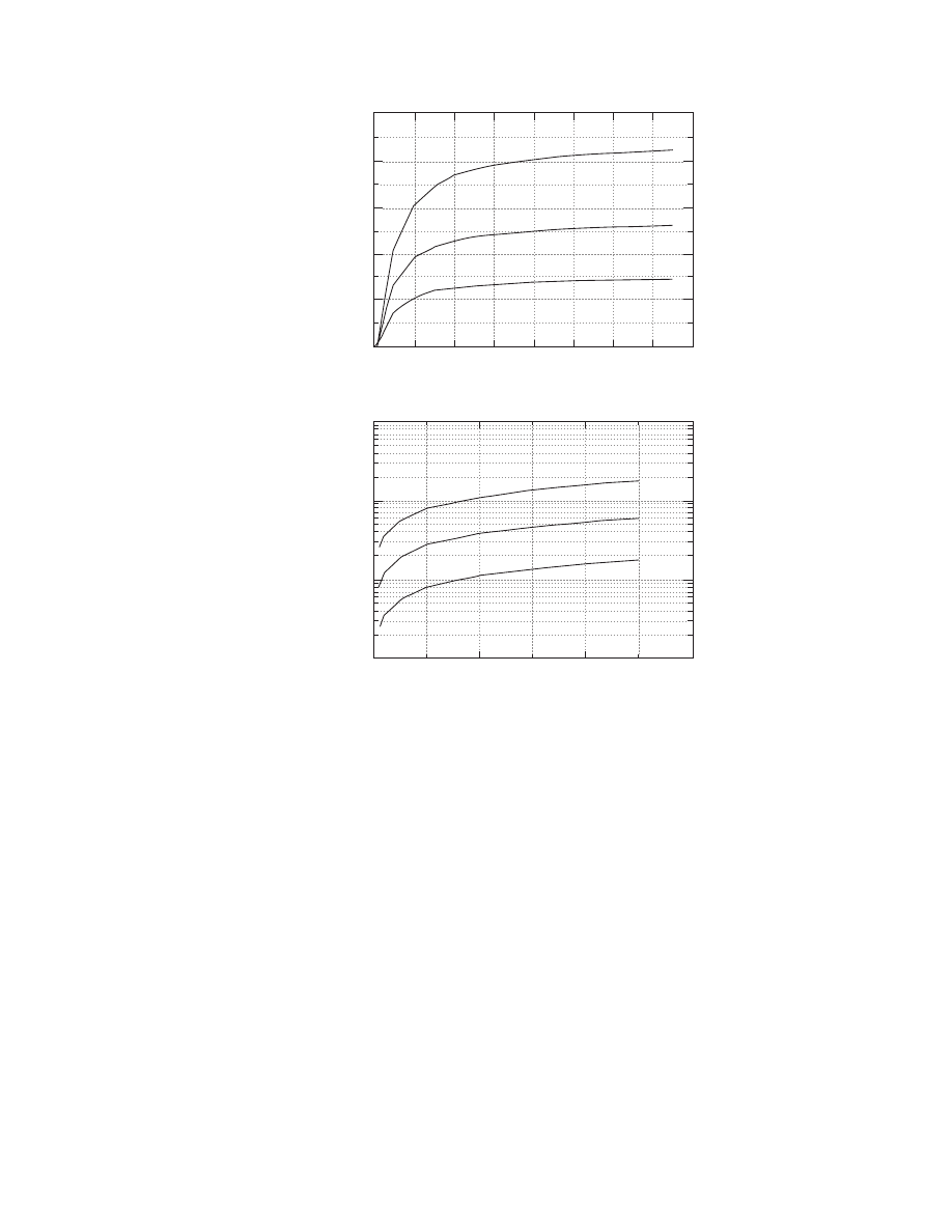
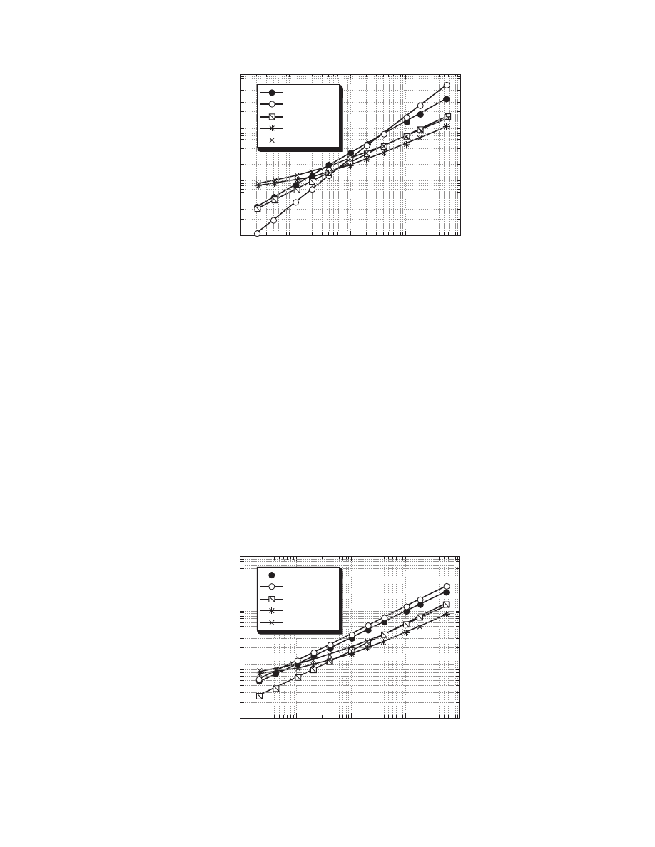
The calculated heat and mass transfer coefficients
using some of the equations presented in Table 4.9 are
plotted versus air velocity with some simplifications in
. These figures can be used
to estimate approximately the heat and mass transfer
coefficients for various dryers. The simplifications
made for the construction of these figures concern
the drying air and material conditions. For instance,
the air temperature is taken as 80 8C, the air humidity
as 0.010 kg/kg db, and the particle size as 10 mm
(typical drying conditions). For other conditions, the
equations of Table 4.9 should be used.
4.4.5 T
HEORETICAL
E
STIMATION
No theory is available for estimating the heat and
mass transfer coefficients using basic thermophysical
properties. The analogy of heat and mass transfer
can be used to obtain mass transfer data from heat
transfer data and vice versa. For this purpose, the
Chilton–Colburn analogies can be used [129]
j
M
¼ j
H
¼ f =2
(4:12)
where f is the well-known Fanning friction factor for
the fluid, and j
H
and j
M
are the heat and mass transfer
factors defined in Table 4.10. Discrepancies of the
above classical analogy have been discussed in
Ref. [143].
In air conditioning processes, the heat and mass
transfer analogy is usually expressed using the Lewis
relationship
h
H
=h
M
¼ c
p
(4:13)
where c
p
(kJ/(kg K)) is the specific heat of air.
TABLE 4.10
Dimensionless Groups of Physical Properties
Name
Definition
Biot for heat transfer
Bi
H
¼ h
H
d/2k
Biot for mass transfer
Bi
M
¼ h
M
d/2rD
Gukhman number
Gu
¼ (T
A
T)/T
A
Heat transfer factor
j
H
¼ StPr
2/3
Mass transfer factor
j
M
¼ (h
M
/u
A
r
A
)Sc
2/3
Nusselt number
Nu
¼ h
H
d/k
A
Prandtl number
Pr
¼ c
p
m
/k
A
Reynolds number
Re
¼ u
A
r
A
d/m
Schmidt number
Sc
¼ m/r
A
D
A
Sherwood number
Sh
¼ h
M
d/r
A
D
A
Stanton number
St
¼ h
H
/u
A
r
A
c
p
c
p
, specific heat (kJ/(kg
K)); d, particle diameter (m); D, diffusivity
in solid (m
2
/s); D
A
, vapor diffusivity in air (m
2
s); «, void fraction in
packed bed; G, mass flow rate of air (kg/(m
2
s)); h
H
, heat transfer
coefficient (kW/(m
2
K)); h
M
, mass transfer coefficient (kg/(m
2
s));
h
VH
, volumetric heat transfer coefficient (kW/(m
3
K)); h
VH
,
volumetric mass transfer coefficient (kg/(m
3
s)); k, thermal
conductivity of solid (kW/(m
K)); k
A
, thermal conductivity of air
(kW/(m
K)); m, dynamic viscosity of air (kg/(ms)); Nu’, Nu’ ¼ Nu
«
/(1
«); Q
A
, density of air (kg/m
3
); Re’, Re’
¼ Re (1 «); Re
s
, Re
based on u
s
instead of u; T
A
, air temperature (8C); T, material
temperature (8C); u
A
, air velocity (m/s); u
s
, air velocity for
incipient spouting (m/s).
ß
2006 by Taylor & Francis Group, LLC.
4.5 DRYING CONSTANT
4.5.1 D
EFINITION
The transport properties discussed above (moisture
diffusivity, thermal conductivity, interface heat, and
mass transfer coefficients) describe completely the
drying kinetics. However, in the literature sometimes
(mainly in foods, especially in cereals) instead of the
above transport properties, the drying constant K is
used. The drying constant is a combination of these
transport properties.
The drying constant can be defined using the so-
called thin-layer equation. Lewis suggested that dur-
ing the drying of porous hygroscopic materials, in the
falling rate period, the rate of change in material
moisture content is proportional to the instantaneous
difference between material moisture content and the
expected material moisture content when it comes
into equilibrium with the drying air [144]. It is as-
sumed that the material layer is thin enough or the
air velocity is high so that the conditions of the drying
air (humidity, temperature) are kept constant through-
out the material. The thin-layer equation has the
following form:
dX =dt ¼ K(X Xe)
(4:14)
where X (kg/kg db) is the material moisture content,
Xe (kg/kg db) is the material moisture content in
equilibrium with the drying air, and t (s) is the time.
Packed
Fluidized
Rotary
Spray
Pneumatic
0.001
0.01
0.1
1
1
10
10
100
1000
Heat
transfer
coefficient
(W/m
2
K)
FIGURE 4.8 Heat transfer coefficients versus air velocity for some dryers (particle size 10 mm; drying conditions T
A
¼ 808C,
X
A
¼ 10 g/kg db).
Packed
Fluidized
Rotary
Spray
Pneumatic
0.001
0.001
0.01
0.01
0.1
0.1
1
1
10
Heat
transfer
coefficient
(W/(m
2
s))
FIGURE 4.9 Mass transfer coefficients versus air velocity for some dryers (particle size 10 mm; drying conditions T
A
¼
808C, X
A
¼ 10 g/kg db).
ß
2006 by Taylor & Francis Group, LLC.

A review of several other thin-layer equations can be
found in Refs. [76,145].
constitutes an effort toward a uni-
fied description of the drying phenomena regardless
of the controlling mechanism. The use of similar eq-
uations in the drying literature is ever increasing. It is
claimed, for example, that they can be used to esti-
mate the drying time as well as for the generalization
of the drying curves [6].
The drying constant K is the most suitable quan-
tity for purposes of design, optimization, and any
situation in which a large number of iterative model
calculations are needed. This stems from the fact that
the drying constant embodies all the transport prop-
erties into a simple exponential function, which is the
solution of Equation 4.14 under constant air condi-
tions. On the other hand, the classical partial differ-
ential equations, which analytically describe the four
prevailing transport phenomena during drying (in-
ternal–external, heat–mass transfer), require a lot of
time for their numerical solution and thus are not
attractive for iterative calculations.
4.5.2 M
ETHODS OF
E
XPERIMENTAL
M
EASUREMENT
The measurement of the drying constant is obtained
from drying experiments. In a drying apparatus, the
air temperature, humidity, and velocity are controlled
and kept constant, whereas the material moisture
content is monitored versus time. The drying constant
is estimated by fitting the thin-layer equation to ex-
perimental data.
4.5.3 F
ACTORS
A
FFECTING THE
D
RYING
C
ONSTANT
The drying constant depends on both material and
air properties as it is a phenomenological property
representative of several transport phenomena. So, it
is a function of material moisture content, temperature,
and thickness, as well as air humidity, temperature,
and velocity.
Some relationships describing the effect of the
above factors on the drying constant are presented in
Table 4.11. Equation T11.1 and Equation T11.2 are
Arrhenius-type equations, which take into account the
temperature effect only. The effect of water activity
can be considered by modifying the activation energy
(Equation T11.1) on the preexponential factor (Equa-
tion T11.2). Equation T11.1 and Equation T11.2 con-
sider the same factors in a different form. Equation
T11.4 takes into account only the air velocity effect,
whereas Equation T11.5 considers all the factors
affecting the drying constant.
eter values for typical equations of Table 4.11.
Equation T11.2 and Equation T11.5 were applied
to shelled corn [150] and to green pepper [35], respect-
ively, and the results are presented in
. The
effects of air temperature and velocity, as well as
particle dimensions, are shown for green pepper
drying, whereas the air temperature and the small
air–water activity effects are shown for the low air
temperature drying of wheat.
4.5.4 T
HEORETICAL
E
STIMATION
It is impossible to estimate an empirical constant
using theoretical arguments. The estimation of an
TABLE 4.11
Effect of Various Factors on the Drying Constant
Equation No.
Materials of Application
Equation
Ref.
T11.1a
Grains, barley, various
tropical agricultural products
K(T
A
)
¼ b
0
exp[
b
1
/T
A
]
75,146,147
T11.1b
Barley, wheat
K(T
A
)
¼ b
0
exp[
b
1
/(b
2
þ b
3
T
A
)]
148
T11.2a
Melon
K(a
w
, T
A
)
¼ b
0
exp[
(b
1
þ b
2
a
w
)/T
A
]
149
T11.2b
Corn, shelled
K(a
w
, T
A
)
¼ b
0
exp(
b
1
a
w
) exp[
b
2
/(b
3
þ b
4
T
A
)]
150
T11.3a
Rice
K(a
w
, T
A
)
¼ b
0
þ b
1
T
A
b
2
a
w
151
T11.3b
Wheat
K(a
w
, T
A
)
¼ b
0
þ b
1
T
A
2
b
2
a
w
152
T11.4
Carrot
K(u
A
)
¼ exp(b
1
þ b
2
ln u
A
)
153
T11.5
Potato, onion, carrot, pepper
K(a
w
, T
A
, d, u
A
)
¼ b
0
a
w
b
1
T
A
b
2
d
b
3
u
A
b
4
35
K, Drying constant; T
A
, temperature; u
A
, air velocity; a
w
, water activity; d, particle diameter; b
1
, parameters.
ß
2006 by Taylor & Francis Group, LLC.

empirical constant using theoretical arguments has
little, if any, meaning. Nevertheless, if we assume
that for some drying conditions the controlling mech-
anism is the moisture diffusion in the material, then
the drying constant can be expressed as a function
of moisture diffusivity. For slabs, for example, the
following equation is valid:
K
¼ p
2
D=L
2
(4:15)
40
°C
70
°C
100
°C
Air velocity (m/s)
Green pepper
Shelled corn
Drying
constant
(1/h)
0
0
1
1 cm
1.5 cm
1
2
2
3
3
4
4
5
5
6
Temperature (
°C)
Drying
constant
(1/h)
10
0
20
0.2
30
40
0.6
50
0.4
60
0.8
70
a
w
=
0.10
0.30
0.60
FIGURE 4.10 Effect of various factors on the drying constant. Data for green pepper are from Kiranoudis, C.T., Maroulis,
Z.B., and Marinos-Kouris, D., Drying Technol., 10(4), 995, 1992 and data for shelled corn are from Westerman, P.W., White,
G.M., and Ross, I.J., Trans. ASAE, 16, 1136, 1973.
TABLE 4.12
Application Examples
Material
Equation
Constants
Ref.
Shelled corn
K
¼ b
0
exp(
b
1
a
w
) exp[
b
2
/(b
3
þ b
4
T
A
)]
0.1 < a
w
<
0.6, 23.5 < T
A
<
56.98C
b
0
¼ 170/s, b
1
¼ 1.15, b
2
¼ 8259,
b
3
¼ 492, b
4
¼ 1.8/8C
150
Green pepper
K
¼ b
0
X
A
b
1
T
A
b
2
d
b
3
u
A
b
4
0.006 < X
A
<
0.022 kg/kg db,
60 < T
A
<
908C, 0.005 < d < 0.015 m, 3 < u
A
<
5 m/s
b
0
¼ 1.11 · 10
8
/s, b
1
¼ 9.03 · 10
2
,
b
2
¼ 1.54, b
3
¼ 0.982, b
4
¼ 0.293
35
Source: From Brunauer, S., Deming, L.S., Deming, W.E., and Teller, E., Am. Chem. Soc. J., 62, 1723, 1940. With permission.
ß
2006 by Taylor & Francis Group, LLC.
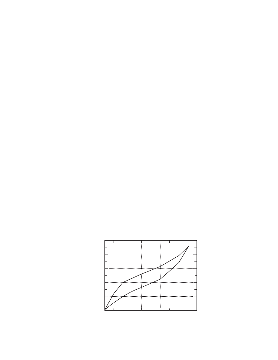
where D (m
2
/s) is the effective diffusivity and L (m) is
the thickness of the slab.
4.6 EQUILIBRIUM MOISTURE CONTENT
4.6.1 D
EFINITION
A knowledge of the state of thermodynamic equilib-
rium between the surrounding air and the solid is a
basic prerequisite for drying, as it is for any similar
mass transfer situation.
The moisture content of the material when it
comes into equilibrium with drying air is a useful
property included in most drying models. The rela-
tion between equilibrium material moisture content
and the corresponding water activity for a given tem-
perature is known as the sorption isotherm. The water
activity a
w
at the pressures and temperatures that
usually prevail during drying is equal to the relative
humidity of air.
The equilibrium moisture of a material can be
attained either by adsorption or by desorption, as
expressed by the respective isotherms of Figure 4.11.
The usually observed deviation of the two curves is
due to the phenomenon of hysteresis, which has not
yet been quantitatively described. Many explanations
for the phenomenon have been put forth that con-
verge in that there are more active sites during the
desorption than during adsorption. It is clear from
Figure 4.11 that the desorption isotherm is the curve
to use for the process of drying.
In essence, the sorption isotherms express the min-
imum value of material moisture content that can be
reached by a solid during drying in relation to the
relative humidity of the drying air. On the basis of
such isotherms, the equilibrium material moisture
content can be calculated. Such equilibrium values
are necessary for the formulation of the mass transfer
driving forces.
Moreover, the isotherms determine the proper
storage environment and the packaging conditions,
especially for foods. Through the isotherms, the isos-
teric heat of sorption can be determined and, hence an
accurate prediction can be made of the energy re-
quirements for the drying of a solid. The utility of
the isotherm is extended to the determination of the
moisture sorption mechanism as well as to the degree
of bound water.
Brunauer et al. [154] classified the sorption iso-
therms into five different types (
). The
sorption isotherms of the hydrophilic polymers, such
as natural fibers and foods, are of type II. The iso-
therms of the less hydrophilic rubbers, plastics, syn-
thetic fibers, and foods rich in soluble components are
of type III. The isotherms of certain inorganic mater-
ials (such as aluminum oxides) are of type IV. For
many materials, however, the sorption isotherms can-
not be properly classified since they belong to more
than one type.
4.6.2 M
ETHODS OF
E
XPERIMENTAL
M
EASUREMENT
A comprehensive review of existing experimental
measuring methods is given in Refs. [155,156]. Sorp-
tion isotherms can be determined according to two
basic principles, gravimetric and hygrometric.
4.6.2.1 Gravimetric Methods
During the measurement, the air temperature and the
water activity are kept constant until the moisture
content of the sample attains the constant equilibrium
Water activity
Equilibrium
material
moisture
content
Desorption
Adsorption
FIGURE 4.11 Hysteresis between adsorption and desorption isotherms.
ß
2006 by Taylor & Francis Group, LLC.
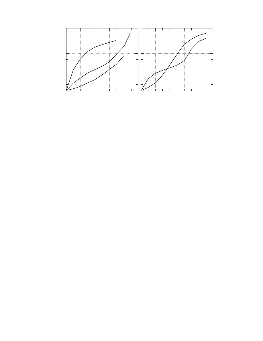
value. The air may be circulated (dynamic methods)
or stagnant (static). The material weight may be regis-
tered continuously (continuous methods) or discon-
tinuously (discontinuous methods).
4.6.2.2 Hygr ometric Methods
During the measurement, the material moisture con-
tent is kept constant until the surrounding air attains
the constant equilibrium value. The air–water activity
is measured via hygrometer or manometer.
The working group in the COST 90bis Project has
developed a reference material (microcrystalline cel-
lulose, MCC) and a reference method for measuring
water sorption isotherms, and conducted a collabora-
tive study to determine the precision (repeatability
and reproducibility) with which the sorption isotherm
of the reference material may be determined by
the reference method. A detailed procedure for the
resulting standardized method was presented, and
the factors influencing the results of the method
were discussed [157–159].
4.6.3 D
ATA
C
OMPILATION
A large volume of data of equilibrium moisture con-
tent appears in the literature. Data for more than 35
polymeric materials, such as natural fibers, proteins,
plastics, and synthetic fibers, are given in Ref. [8].
Isotherms for 32 materials (organic and inorganic)
are also given in Ref. [92]. The literature is especially
rich in sorption isotherms of foods due to the fact that
the value of water activity is a critical parameter for
food preservation safety and quality.
A bibliography on sorption isotherms of food
materials is presented in Ref. [160]. The collection
comprises 2200 references, including about 900 pa-
pers with information on equilibrium moisture con-
tent of foods in defined environments. The papers are
listed alphabetically according to the names of the
first author, but they are also grouped according to
product.
Additional bibliographies should also be men-
tioned. The Handbook of Food Isotherms contains
more than 1000 isotherms, with a mathematical de-
scription of over 800 [161]. About 460 isotherms were
obtained from the monograph of Ref. [162]. Data on
sorption properties of selected pharmaceutical mater-
ials are presented in Ref. [98].
4.6.4 F
ACTORS
A
FFECTING THE
E
QUILIBRIUM
M
OISTURE
C
ONTENT
Equilibrium material moisture content depends upon
many factors, among which are the chemical compos-
ition, the physical structure, and the surrounding air
conditions. A large number of equations (theoretical,
semiempirical, empirical) have been proposed, none
of which, however, can describe the phenomenon of
hysteresis. Another basic handicap of the equations is
that their applicability is not satisfactory over the
entire range of water activity (0 # a
w
#
1).
lists the best-known isotherm equa-
tions. The Langmuir equation can be applied in type I
isotherm behavior. The Brunauer–Emmet–Tetter
(BET) equation has been successfully applied to al-
most all kinds of materials, but especially to hydro-
philic polymers for a
w
<
0.5. The Halsey equation
is suitable for materials of types I, II, and III. The
Henderson equation is less versatile than that of
Halsey. For cereal and other field crops, the Chung
Water activity
Equilibrium
material
moisture
content
I
II
III
IV
V
FIGURE 4.12 The five types of isotherms. (From Brunauer, S., Deming, L.S., Deming, W.E., and Teller, E., Am. Chem. Soc.
J., 62, 1723, 1940.)
ß
2006 by Taylor & Francis Group, LLC.

and Pfost equation is considered suitable, whereas
that of Iglesias and Chirife has been successfully ap-
plied on isotherms of type III (i.e., foods rich in
soluble components).
The Guggenheim–Anderson–de Boer (GAB) equa-
tion is considered as the most versatile model, capable
of application to situations over a wide range of water
activities (0.1 < a
w
<
0.9) and to various materials
(inorganic, foods, etc.). The GAB equation is probably
the most suitable for process analysis and design of
drying because of its reliability, its simple mathematical
form, and its wide use (with materials and water activ-
ity ranges). Table 4.14 lists parameter values of the
GAB equation for some foods.
Two selected food materials are presented as an
. Potatoes exhibit a typical
behavior. Equilibrium material moisture content is
increased [172]. Raisins, on the other hand, exhibit
an inverse temperature effect at large water activities
[173]. As shown in Figure 4.13, potatoes and raisins
exhibit sorption isotherms of types II and III, respect-
ively.
The isotherms at 25 8C for some organic and inor-
ganic materials are presented in
Figure 4.14, one can observe the various isotherm
types, like type I for activated charcoal and silica
gel, type II for leather, type III for soap, and so on.
Various regression analysis methods for fitting
the above equations to experimental data have
been discussed in the literature. The direct nonlinear
regression exhibits several advantages over indirect
nonlinear regression [173]. Linear regression, on the
other hand, can give highly erroneous results and
should be avoided [174]. When there exist differences
in the variance of the data, the direct nonlinear
weighted regression method should be used [175].
4.7 SIMULTANEOUS ESTIMATION OF HEAT
AND MASS TRANSPORT PROPERTIES
FROM DRYING EXPERIMENTS
4.7.1 P
RINCIPLES OF
E
STIMATION
In the previous sections, methods of experimental
determination of heat and mass transport properties
have been discussed. These methods use special ap-
paratus and are based on the equation of definition of
the corresponding property. This section discusses the
experimental determination of these properties from
drying experiments. Some relevant techniques have
been already discussed by Molnar [125]. However, a
generalized method based on model-building tech-
niques is presented here. The method uses a drying
experimental apparatus and estimates the heat and
mass transport properties as parameters of a drying
model that incorporates these properties [28,43,176–
180]. An outline of the method is described below.
First, an experimental drying apparatus is used. In
such an apparatus, the air passes through the drying
material and the air humidity, temperature, and vel-
ocity are controlled, whereas the material moisture
content and, eventually, the material temperature
are monitored versus time. Second, a mathematical
TABLE 4.13
Effect of Water Activity and Temperature on the
Equilibrium Moisture Content
Equation Name
Equation
Ref.
Langmuir
a
w
1
X
1
b
0
¼
1
b
0
b
1
163
Brunauer–Emmet–
Tetter (BET)
a
w
(1
a
w
)X
¼
1
b
0
b
1
þ
b
1
1
b
0
b
1
a
w
164
Halsey
a
w
¼ exp
b
1
RT
X
b
2
b
3
165
Henderson
1
a
w
¼ exp[b
1
TX
b
2
]
166
Chung and Pfost
ln a
w
¼
b
1
RT
exp (
b
2
X )
167
Chen and Clayton
ln a
w
¼ b
1
T
b
2
exp(
b
3
T
b
2
X)
168
Iglesias and Chirife
ln a
w
¼ exp[(b
1
T
þ b
2
)X
b
3
]
169
Guggenheim–
Anderson–
de Boer (GAB)
X
¼
b
0
b
1
b
2
a
w
(1
b
1
a
w
)(1
b
1
a
w
þ b
1
b
2
a
w
)
b
1
¼ b
10
exp (b
11
=RT
), b
2
¼
b
20
exp (b
21
=RT
)
170,
171
X, Equilibrium material moisture content; a
w
, water activity; T,
temperature; b
1
, parameters.
TABLE 4.14
Application of the Guggenheim–Anderson–de Boer
Model to Some Fruits and Vegetables
Material
b
0
b
10
·
10
5
b
11
b
20
b
21
Potato
8.7
1.86
34.1
5.68
6.75
Carrot
21.2
5.94
28.9
8.03
5.49
Tomato
18.2
1.99
34.5
5.52
6.70
Pepper
21.1
1.46
33.4
5.56
6.56
Onion
20.2
2.30
32.5
5.79
6.43
Raisin
12.5
0.17
22.4
1.77
1.53
Fig
11.7
0.05
25.2
1.77
1.55
Prune
13.3
0.07
23.9
1.82
1.65
Apricot
15.1
0.11
21.1
2.13
2.05
Source: From Kiranoudis, C.T., Maroulis, Z.B., Tsami, E., and
Marinos-Kouris, D., J. Food Eng., 20(1), 55, 1992; Maroulis,
Z.B., Tsami, E., Marinos-Kouris, D., and Saravacos, G.D.,
J. Food Eng., 7(1), 63, 1988.
ß
2006 by Taylor & Francis Group, LLC.
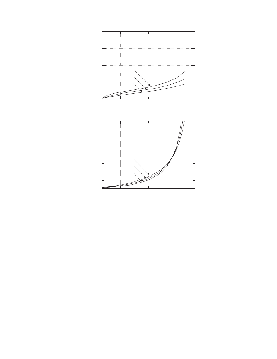
model that takes into account the controlling
mechanisms of heat and mass transfer is considered.
This model includes the heat and mass transport
properties as model parameters or, even more, in-
cludes the functional dependence of the relevant fac-
tors on the transport properties. Third, a regression
analysis procedure is used to obtain the transport
properties as model parameters by fitting the model
to experimental data of material moisture content and
temperature.
Theoretically, all the properties describing the
drying kinetics could be estimated simultaneously.
We can define the drying kinetics (in an analogous
manner to reaction kinetics) as the dependence of
factors affecting the drying on the drying rate. Drying
is not a chemical reaction, but it involves simultaneous
heat and mass transfer phenomena. Consequently, the
properties describing these phenomena describe the
drying process as well.
If, for example, the phenomena considered are
The moisture diffusion in the solid toward its
external surface
The vaporization and convective transfer of the
vapor into the airstream
The conductive heat transfer within the solid mass
The convective heat transfer from the air to the
solid’s surface
then the following properties describe the drying
kinetics:
Effective moisture diffusivity
Air boundary mass transfer coefficient
Equilibrium
material
moisture
content
(%db)
0
0
20
40
60
60
⬚C
45
⬚C
30
⬚C
80
0.2
0.4
0.6
0.8
1
Water activity
Equilibrium
material
moisture
content
(%db)
0
0
20
40
60
60
°C
45
°C
30
°C
80
0.2
0.4
0.6
0.8
1
Water activity
Potatoes
Sultana raisins
FIGURE 4.13 Effect of air–water activity and temperature on equilibrium material moisture content for two foods. (Data for
potatoes from Kiranoudis, C.T., Maroulis, Z.B., Tsami, E., and Marinos-Kouris, D., J. Food Eng., 20(1), 55, 1992 and data
for sultana raisins from Maroulis, Z.B., Tsami, E., Marinos-Kouris, D., and Saravacos, G.D., J. Food Eng., 7(1), 63, 1988.)
ß
2006 by Taylor & Francis Group, LLC.
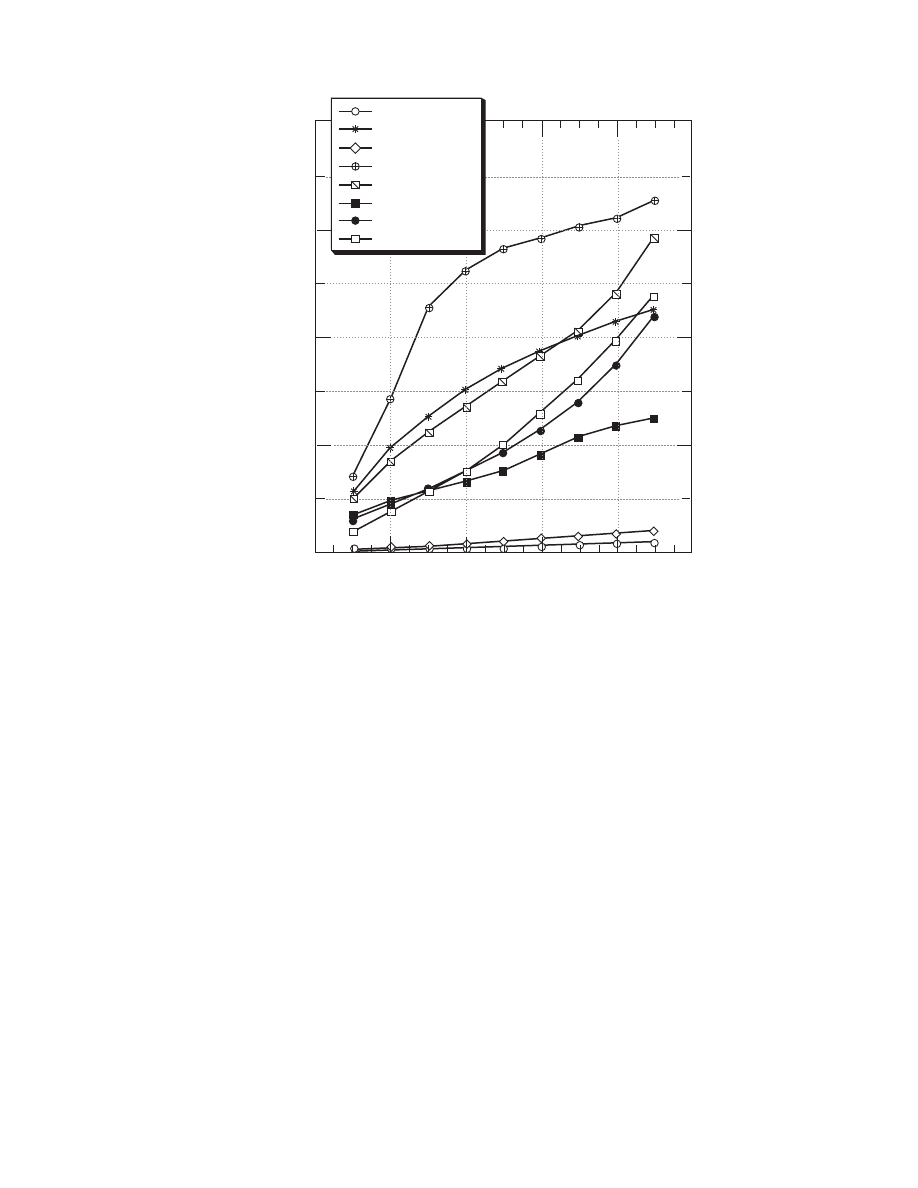
Effective thermal conductivity
Air boundary heat transfer coefficient
and consequently they can be estimated.
Alternatively, if the drying constant is assumed to
describe the drying kinetics by the thin-layer equa-
tion, then the drying constant can be estimated using
this method.
4.7.2 E
XPERIMENTAL
D
RYING
A
PPARATUS
A typical drying apparatus is shown in
The apparatus consists of two parts, the air con-
ditioning section and the measuring section. The
air conditioning section includes the heater, the
humidifier, and the fan, which are handled via a
temperature, a humidity, and a flow controller, re-
spectively. In the measuring section, the air proper-
ties, that is, temperature, humidity, and velocity, as
well as the material properties (weight and tempera-
ture) are continuously recorded. The use of a computer
for online measurement and control is preferable.
4.7.3 T
HE
D
RYING
M
ODEL
An information flow diagram for a drying model
appropriate for this method is shown in
.
This model can calculate the material moisture con-
tent and temperature as a function of position and
time whenever the air humidity, temperature, and
velocity are known as a function of time, together
with the model parameters. If the model takes into
account the controlling mechanisms of heat and mass
transfer, then the transport properties (moisture dif-
fusivity, thermal conductivity, boundary heat and
mass transfer coefficients) are included in the model
as parameters. If the dependence of drying conditions
(material moisture content, temperature, and thick-
ness, as well as air humidity, temperature, and vel-
ocity) on transport properties is also considered, then
the constants of the relative empirical equations are
considered as model parameters. In Figure 4.16 the
part of the model that contains equations for the heat
and mass transfer phenomena is termed the process
model, whereas the equations describing the dependence
Equilibrium
material
moisture
content
(%db)
0
0
20
40
10
30
0.2
0.4
0.6
0.8
1
Water activity
Asbestos fiber
Silica gel
Domestic coke
Activated charcoal
Leather
Glue
Wood
Soap
FIGURE 4.14 Equilibrium material moisture content for some organic and inorganic materials. (Data from Perry, R.H. and
Chilton, C.H., Chemical Engineers’ Handbook, 4th and 5th ed., McGraw-Hill, New York, 1963, 1973.)
ß
2006 by Taylor & Francis Group, LLC.
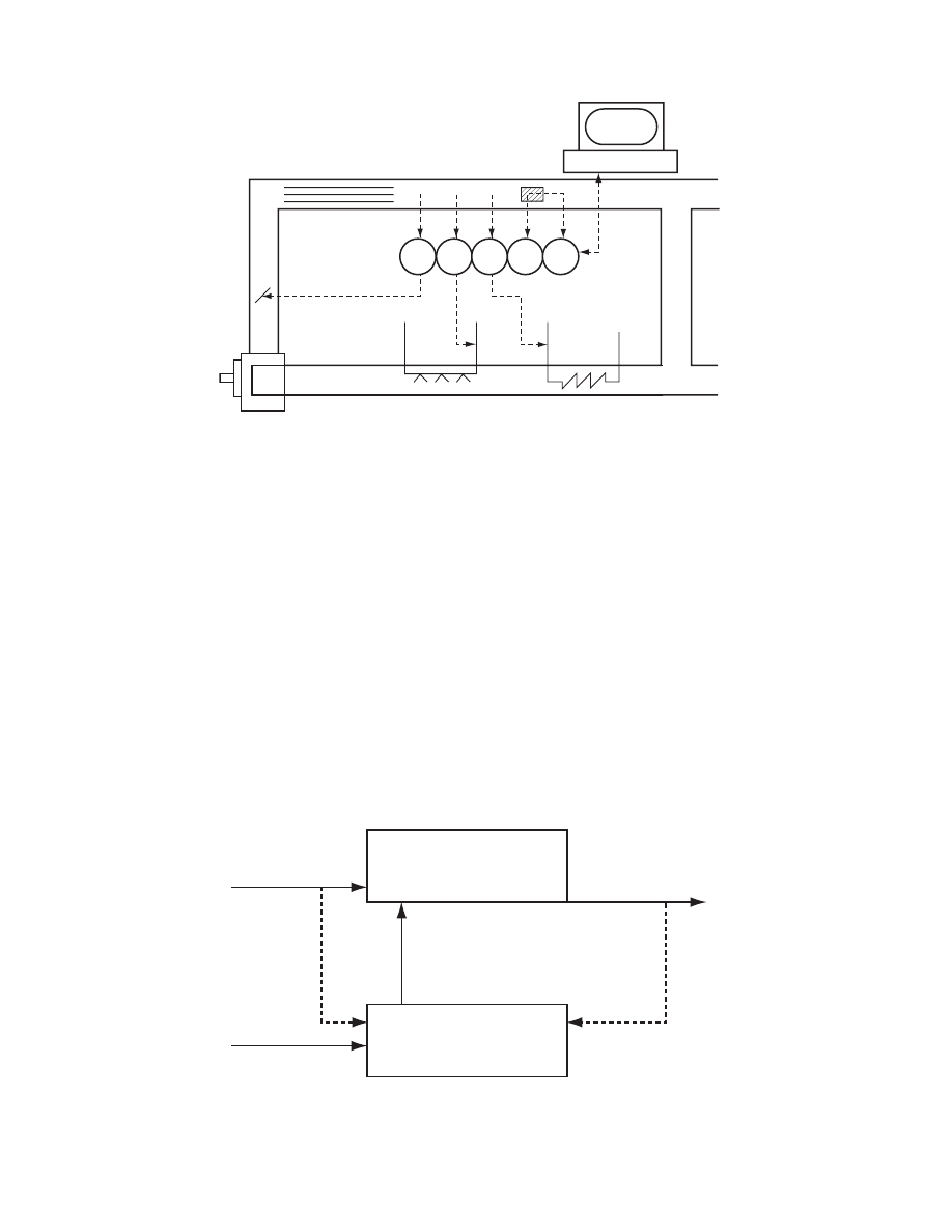
of drying conditions on transport properties form the
properties model.
In the process model, each mechanism of heat and
mass transfer is expressed using a driving force and a
transport property as a coefficient of proportionality
between the rate and the corresponding driving force.
In the properties model, several formulas can be con-
sidered. Some assumptions have been suggested in the
previous sections.
4.7.4 R
EGRESSION
A
NALYSIS
The parameters of a model can be estimated by fitting
the model to experimental data [181,182]. Using the
, two regression analysis pro-
cedures can be applied [43]: transport properties esti-
mation and transport properties equations estimation.
4.7.4.1 Tran sport Prop erties Estima tion
It is assumed that during the drying experiments the
drying conditions are not varying very much with
time, and the transport properties can be considered
constant (not functions of the drying conditions). The
transport properties are estimated as parameters of
the process model by fitting it to experimental data.
Only the properties of the controlling mechanisms
can be obtained. Consequently, the precision and
4
3
2
6
5
7
1
FCR HCR TCR
WR
TR
PC
Air conditioning section
Measuring section
FIGURE 4.15 Typical experimental drying apparatus: (1) sample; (2) air recirculating duct; (3) heater; (4) humidifier; (5) fan;
(6) valve; (7) straighteners; FCR, airflow control and recording; HCR, air humidity control and recording; TCR, air
temperature control and recording; WR, sample weight recording; TR, sample temperature recording; PC, personal
computer, for on-line measurement and control.
Drying conditions
(air humidity,
temperature and velocity)
Model results
(material moisture content
and temperature)
Process model
(heat and mass transfer equations)
Empirical constants
Transport properties model
(empirical equations describing
the effect of various factors
on transport properties)
Transport properties
(moisture diffusivity, thermal conductivity,
heat and mass transfer coefficients)
FIGURE 4.16 Model information flow diagram.
ß
2006 by Taylor & Francis Group, LLC.

correlations of the estimates should be examined. A
model discrimination procedure is suggested to dis-
card the noncontrolling mechanisms.
4.7.4.2 Tran sport Prop erties Eq uations Estima tion
Several empirical equations describing the depend-
ence of transport properties on various factors are
tested using a model discrimination procedure. The
constants of the empirical equations are estimated as
parameters of the total model (process model plus
properties model) by fitting it to experimental data.
The information flow diagram for the regression
analysis proposed is shown in Figure 4.17.
4.7.5 A
PPLICATION
E
XAMPLE
The method described above is applied to a wide set
of experimental data in potato drying [43].
4.7.5.1 Experimental Drying Apparatus
An experimental drying apparatus similar to that
shown in
was used [35]. In each experi-
ment, the air–water activity, temperature, and vel-
ocity were controlled, and the material moisture
content and temperature were monitored versus
time. A total number of 100 experiments were per-
formed for three different particle dimensions (5, 10,
and 15 mm) at five air temperature (60, 65, 70, 75, and
808C), three air velocities (3, 4, and 5 m/s) and at air
humidity ranging from 6 to 22 g/kg db.
4.7.5.2 Drying Model
A mathematical drying model involving simultaneous
heat and mass transfer is considered for the analysis
[43]. The model considered has the following form:
Moisture diffusion into the solid
@
(X )=@t
¼ r(DrX )
(4:16)
D
¼ a
0
exp (
a
1
=X
) exp (
a
2
=T
)
(4:17)
Boundary layer vapor transfer
(DrX ) ¼ h
M
(a
we
a
w
)
(4:18)
h
M
¼ c
0
X
c
1
A
T
c
2
A
u
c
3
A
(4:19)
Heat conduction in the solid
@
(h
s
)=@t
¼ r(krT)
(4:20)
k
¼ b
0
exp (
b
1
=X
) exp (
b
2
=T
)
(4:21)
Boundary layer heat transfer
(krT) ¼ h
H
(T
T
A
)
DH
s
h
M
(a
we
a
w
)
(4:22)
h
H
¼ d
0
X
d
1
A
T
d
2
A
u
d
3
A
(4:23)
where X and T are the material moisture content and
temperature, respectively, u
A
, a
w
, and T
A
are the air
velocity, water activity, and temperature, respectively.
The thermophysical and thermodynamic properties,
material density r, material specific enthalpy h
s
, heat
of vaporization of water DH
s
, and equilibrium air–
water activity a
we
are known functions of material
moisture content and temperature.
The transport properties, moisture diffusivity D,
and thermal conductivity k are functions of material
moisture content and temperature, whereas heat and
mass transfer coefficients, h
H
, h
M
, are functions of air
velocity, water activity, and temperature.
The following adjustable constants are introduced
to the relevant properties model: a
i
, b
i
, c
i
, d
i
.
Measured
input
variables
Measured
output
variables
Computed
output
variables
Regression
analysis
Parameter
estimates
Experimental
apparatus
Process model
(and enventually
properties model)
FIGURE 4.17 Regression analysis information flow diagram.
ß
2006 by Taylor & Francis Group, LLC.

4.7.5.3 Regression Analysis
If X
i
and T
i
are the experimental values of material
moisture content and temperature and X
i,c
and T
i,c
are the corresponding calculated values using the
mathematical model, then the relative deviations be-
tween experimental and calculated values (relative
residuals) can be defined as follows:
e
Xi
¼ (X
i;c
X
i
)=X
i
(4:24)
e
Ti
¼ (T
i;c
T
i
)=T
i
(4:25)
The relative standard deviations between experimen-
tal and calculated values of material moisture content
S
X
and temperature S
T
are defined as follows:
S
X
2
¼ Se
Xi
2
=N
(4:26)
S
T
2
¼ Se
Ti
2
=N
(4:27)
where N is the number of experimental points (includ-
ing different measurements and different experiments).
A linear combination of S
X
and S
T
is used for
parameter estimation and the resulting S
X
, S
T
are
used for model validation [180,182]. The regres-
sion analysis is performed simultaneously on all
experiments.
4.7.5.4 Results
The application of the proposed method proved that:
The moisture diffusivity is a function of material
moisture content and temperature.
The thermal conductivity is high and cannot be
estimated from these experiments.
Heat and mass transfer coefficients are constant in
the region of experimentation.
More specifically, the results obtained are as
follows:
D
¼ 2:94 10
7
m
2
=
s exp(
1:58 10
3
K=T )
exp (
6:72 10
2
kg=kg=X)
(4:28)
h
M
¼ 5:84 10
7
kg=m
2
=
s
(4:29)
h
H
¼ 1:64 10
1
W=m
2
(4:30)
The resulting model calculates the material moisture
content and temperature close to experimental values
and it is considered satisfactory.
4.8 TRANSPORT PROPERTIES OF FOODS
The transport properties of foods received much at-
tention in the literature [184–188]. The main results
presented by Saravacos and Maroulis [188] are sum-
marized in this section. The results refer to moisture
diffusivity and thermal conductivity. Recently pub-
lished values of moisture diffusivity and thermal con-
ductivity in various foods were retrieved from the
literature and were classified and analyzed statistically
to reveal the influence of material moisture content
and temperature. Empirical models relating moisture
diffusivity and thermal conductivity to material mois-
ture content and temperature were fitted to all exam-
ined data for each material. The data were screened
carefully using residual analysis techniques. A prom-
ising model was proposed based on an Arrhenius-type
effect of temperature, which uses a parallel structural
model to take into account the effect of material
moisture content.
4.8.1 M
OISTURE
D
IFFUSIVITY
A total of 175 papers were retrieved from the litera-
ture from which 1773 data were obtained. These data
refer to more than 100 food materials classified into
11 food categories. Among the available data only
19 materials have more than ten data, which come
from more than three publications. The resulting
model is summarized in Table 4.15 and the results
TABLE 4.15
Mathematical Model for Calculating Moisture
Diffusivity in Foods as a Function of Moisture
Content and Temperature
Proposed mathematical model
D
¼
1
1
þX
D
O
exp
E
0
R
1
T
1
T
r
þ
X
1
þ X
D
i
exp
E
i
R
1
T
1
T
r
where D is the moisture diffusivity (m
2
/s), X is the material
moisture content (kg/kg db), T the material temperature (8C),
T
r
is the reference temperature (608C), and R
¼ 0.0083143 is
the ideal gas constant kJ/(mol K)
Adjustable model parameters
D
O
(m
2
/s)
diffusivity at moisture X
¼ 0 and
temperature T
¼ T
r
D
i
(m
2
/s)
diffusivity at moisture X
¼ 1 and
temperature T
¼ T
r
E
0
(kJ/mol)
activation energy for diffusion in dry
material at X
¼ 0
E
i
(kJ/mol)
activation energy for diffusion in wet
material at X
¼ 1
ß
2006 by Taylor & Francis Group, LLC.

of parameter estimation are presented in Table
4.16.
model-calculated values for selected food materials
as a function of moisture content and temperature.
The regression procedure was applied simultan-
eously to all the data of each material, regardless of
the data sources. Thus, the results are not based on the
data of only one author and, consequently, they are of
higher accuracy and general applicability.
The diffusivity parameters D
o
and D
i
of the pro-
posed model vary in the range of 10
10
to 10
8
m
2
/s.
It should be noted that the self-diffusivity of water is
approximately 10
9
m
2
/s, and the moisture diffusivity
in bone-dry food material should be lower (in our
analysis, by a factor of 100).
Low moisture diffusivities are found in nonporous
and sugar-containing foods, whereas higher values of
moisture diffusivity characterize porous food mater-
ials. Diffusivities higher than the self-diffusivity of
water are indicative of vapor diffusion in porous
solids.
The moisture diffusivity increases, in general, with
increasing moisture content. Temperature has a posi-
tive effect, which depends strongly on the food ma-
terial. The energy of activation for diffusion E of
water is, in general, higher in the dry food materials.
Some observed exceptions may be explained by the
prevailing type of diffusion. Thus, lower values of
activation energy for diffusion are expected for porous
foods, where vapor diffusion is important. In general,
temperature has a stronger effect on diffusivity in
liquids and solids than in the gaseous state.
4.8.2 T
HERMAL
C
ONDUCTIVITY
A total of 146 papers were retrieved from the litera-
ture from which 1210 data were obtained. These data
refer to more than 100 food materials classified into
11 food categories. Among the available data only 13
materials have more than 10 data, which come from
more than three publications. This procedure is ap-
plied to these data and the results of parameter
TABLE 4.16
Parameter Estimates of the Proposed Mathematical Model
Material
No. of Papers
No. of Data
D
i
(m
2
/s)
D
O
(m
2
/s)
E
i
(kJ/mol)
E
0
(kJ/mol)
s.d. (m
2
/s)
Cereal products
—Corn
4
26
4.40E-09
0.00E
þ00
0.0
10.4
1.48E-10
Dent
3
15
1.19E-08
0.00E
þ00
49.4
73.1
3.30E-10
Grains
3
28
1.15E-09
6.66E-11
10.2
57.8
3.17E-10
Kernel
4
25
5.87E-10
5.32E-10
0.0
33.8
1.88E-11
Pericarp
3
13
1.13E-09
0.00E
þ00
10.0
5.0
2.34E-11
—Pasta
3
21
1.39E-09
0.00E
þ00
16.2
2.0
7.71E-12
Rice
Kernel
3
12
9.75E-09
0.00E
þ00
12.5
2.0
5.52E-11
—Rough rice
7
35
2.27E-09
0.00E
þ00
12.7
0.7
3.66E-11
—Wheat
6
22
1.94E-09
1.30E-09
0.0
46.3
9.53E-11
Fruits
—Apple
8
39
7.97E-10
1.16E-10
16.7
56.6
1.92E-10
—Banana
4
34
2.03E-09
4.66E-10
9.9
4.6
1.77E-10
Grapes
Seedless
3
32
5.35E-09
0.00E
þ00
34.0
10.4
1.45E-10
—Raisins
3
10
8.11E-10
1.05E-10
21.4
50.1
6.88E-11
Model foods
—Amioca
4
49
1.52E-08
1.52E-08
0.0
33.3
1.02E-09
—Hylon-7
5
48
1.96E-08
1.96E-08
0.0
24.2
3.87E-09
Vegetables
—Carrot
9
90
2.47E-09
1.54E-09
13.9
11.3
1.69E-09
—Garlic
4
22
5.33E-10
1.68E-11
15.4
7.1
7.43E-11
—Onion
4
31
1.45E-08
0.00E
þ00
70.2
10.4
1.58E-09
—Potato
16
106
1.57E-09
4.31E-10
44.7
76.9
4.02E-10
ß
2006 by Taylor & Francis Group, LLC.
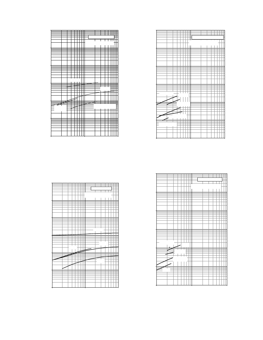
1.E
−12
1.E
−11
1.E
−10
1.E
−09
1.E
−08
1.E
−07
1.E
−06
0.1
1
10
Moisture (kg/kg db)
Diffusivity (m
2
/s)
Grapes,seedless
Fruits
Banana
Apple
Temperature (
⬚C) = 25
Raisins
FIGURE 4.18 Predicted values of moisture diffusivity of
fruits at 258C.
1.E
−12
1.E
−11
1.E
−10
1.E
−09
1.E
−08
1.E
−07
1.E
−06
0.1
10
Moisture (kg/kg db)
Diffusivity (m
2
/s)
Onion
Vegetables
Carrot
Potato
Garlic
Temperature (
⬚C) = 25
FIGURE 4.19 Predicted values of moisture diffusivity of
vegetables at 258C.
1.E
−12
1.E
−11
1.E
−10
1.E
−09
1.E
−08
1.E
−07
1.E
−06
0.1
1
10
Moisture (kg/kg db)
Diffusivity (m
2
/s)
Corn kernel
Cereal products (corn)
Corn grains
Corn dent
Corn
Temperature (
⬚
C) = 25
Corn pericarp
FIGURE 4.20 Predicted values of moisture diffusivity of
corn at 258C.
1.E
−12
1.E
−11
1.E
−10
1.E
−09
1.E
−08
1.E
−07
1.E
−06
0.1
1
10
Moisture (kg/kg db)
Diffusivity (m
2
/s)
Rough rice
Cereal products
Corn
Wheat
Rice kernel
Temperature (
⬚C) = 25
Pasta
FIGURE 4.21 Predicted values of moisture diffusivity of
cereal products at 258C.
ß
2006 by Taylor & Francis Group, LLC.

estimation are presented in Table 4.17 and Table 4.18.
through
present the model-
calculated values for selected food materials as a
function of moisture content and temperature.
Thermal conductivity parameters l
o
and l
i
vary
in the range of 0.05 to 1.0 W/(m K). It should be
noted that the thermal conductivity of air is about
0.026 W/(m K), whereas that of water is 0.60 W/(m
K). Values of thermal conductivity of foods higher
than 0.60 W/(m K) are normally found in frozen food
materials ( l
ice
¼ 2 W/(m K)).
The thermal conductivity increases, in general,
with increasing moisture content. Temperature has a
positive effect, which depends strongly on the food
material. The energy of activation for heat conduc-
tion E is, in general, higher in dry food materials.
ACKNOWLEDGMENT
The authors are grateful to Professor G.D. Saravacos
and Dr. J.A. Palyvos for their valuable suggestions.
NOMENCLATURE
A
o
effective surface area for heat and mass transfer,
m
2
A’ vibration amplitude, m
a
i
and in
, various units of measure
a
w
air–water activity
TABLE 4.17
Mathe matical Model for Calcul ating The rmal
Conduct ivity in Foods as a Fu nction of Moisture
Conten t and Temper ature
Proposed mathematical model
l
¼
1
1
þ X
l
0
exp
E
0
R
1
T
1
T
r
þ
X
1
þ X
l
i
exp
E
i
R
1
T
1
T
r
where l is the thermal conductivity (W/(m K)), X is the material
moisture content (kg/kg db), T the material temperature (8C),
T
r
¼ 60 8C a reference temperature, and R ¼ 0.0083143 the ideal
gas constant kJ/(mol K)
Adjustable model parameters
l
0
(W/(m K)) thermal conductivity at moisture X
¼ 0 and
temperature T
¼ T
r
l
i
(W/(m K)) thermal conductivity at moisture X
¼ 1 and
temperature T
¼ T
r
E
0
(kJ/mol) activation energy for heat conduction in dry material at
X
¼ 0
E
i
(kJ/mol) activation energy for heat conduction in wet material at
X
¼ 1
TABLE 4.18
Param eter Estima tes of the Proposed Mathe mat ical Mod el
Material No. of Papers No. of Data l
i
(W/(m K)) l
0
(W/(m K)) E
i
(kJ/mol) E
0
(kJ/mol) s.d. (W/(m K))
Cereal products
Corn 3 15 1.580 0.070 7.2 5.0 0.047
Fruits
Apple 12 68 0.589 0.287 2.4 11.7 0.114
Orange 4 13 0.642 0.106 1.3 0.0 0.007
Pear 5 15 0.658 0.270 2.4 1.9 0.016
Model foods
Amioca
5
29
0.718
0.120
3.2
14.4
0.037
Starch
4
24
0.623
0.243
0.3
0.4
0.006
Hylon
3
21
0.800
0.180
9.9
0.072
Vegetables
Potato
12
37
0.611
0.049
0.0
47.0
0.059
Tomato
5
28
0.680
0.220
0.2
5.0
0.047
Dairy
Milk
5
33
0.665
0.212
1.7
1.9
0.005
Meat
Beef
6
37
0.568
0.280
2.2
3.2
0.017
Other
Rapeseed
3
35
0.239
0.088
3.6
0.6
0.023
Baked products
Dough
3
15
0.800
0.273
2.7
0.0
0.183
ß
2006 by Taylor & Francis Group, LLC.
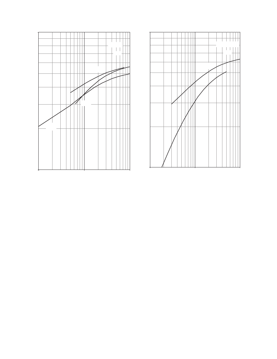
a
we
equilibrium air–water activity
b
i
, various units of
measure
Bi
H
Biot number for heat transfer (
)
Bi
M
Biot number for mass transfer (see Table 4.10)
c
i
, various units of
measure
c
p
specific heat, kJ/(kg
K)
DH
s
latent heat of vaporization, kJ/kg
d particle diameter, m
d
i
, various units of
measure
D diffusivity in solids, m
2
/s
D
A
vapor diffusivity in air, m
2
/s
D ’ diameter of spouted bed, m
db dry base
D
O
, m
2
/s
E activation energy in Arrhenius equation, kJ/
kmol
e
Ti
relative deviation between experimental and
calculated values of material temperature, 8C
e
Xi
relative deviation between experimental and
calculated values of material moisture content,
kg/kg db
F constant (
)
f friction factor
f’ vibration frequency, 1/s
G mass flow rate of air, kg/(m
2
s)
Gu Gukhman number (see Table 4.10)
h
H
heat transfer coefficient, kW/(m
2
K)
h
M
mass transfer coefficient, kg/(m
2
s)
H
0
static bed height for spouted beds, m
h
s
specific enthalpy, kJ/kg
h
VH
volumetric heat transfer coefficient, kW/(m
3
K)
h
VM
volumetric mass transfer coefficient kg/(m
3
s)
J rate of mass transfer, kg/s
j
H
heat transfer factor (see Table 4.10)
j
M
mass transfer factor (see Table 4.10)
K drying constant, 1/s, 1/h
k effective thermal conductivity, kW/(m
K)
k
A
thermal conductivity of air, kW/(m
K)
k
i
thermal conductivity of phase i, kW/(m
2
K)
L slab thickness, m
0.1
0.1 1
1
10
Moisture (kg/kg db)
Conductivity (W/(m K))
Fruits
Pear
Orange
Apple
25
⬚C
FIGURE 4.22 Predicted values of thermal conductivity of
fruits at 258C.
0.1
1
0.1
1
10
Moisture (kg/kg db)
Conductivity (W/(m K))
Vegetables
Tomato
Potato
25
⬚C
FIGURE 4.23 Predicted values of thermal conductivity of
vegetables at 258C.
ß
2006 by Taylor & Francis Group, LLC.
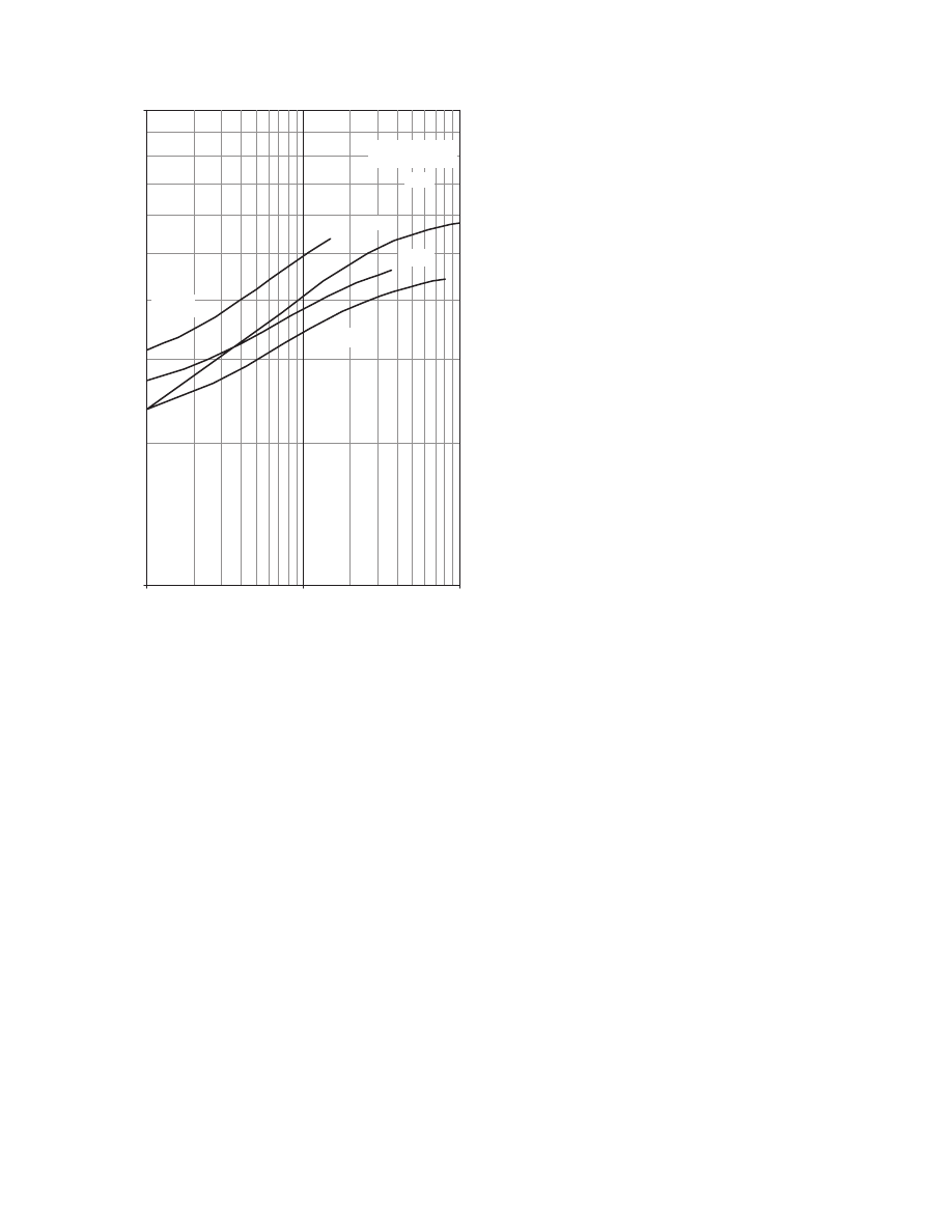
N number of measurements
Nu Nusselt number (
)
Nu ’ Nu ’
¼ Nu «/(1 – «)
Pr Prandtl number (see Table 4.10)
Q rate of heat transfer, kW/s
R gas constant, kJ/(kmol
K)
Re Reynolds number (see Table 4.10)
Re’ Re’
¼ Re (1 «)
Re
s
Re based on u
s
instead of u
A
Sc Schmidt number (see Table 4.10)
Sh Sherwood number (see Table 4.10)
St Stanton number (see Table 4.10)
S
T
standard deviation between experimental and
calculated values of material temperature, 8C
S
X
standard deviation between experimental and
calculated values of material moisture content,
kg/kg db
t time, s
T
A
air temperature, 8C
T material temperature, 8C
T
i
experimental value of material temperature
during measurement i, 8C
T
i,c
calculated value of material temperature during
measurement i, 8C
u
A
air velocity, m/s
u
s
air velocity for incipient spouting, m/s
V total volume of the material, m
3
wb wet base
X material moisture content, kg/kg db
X
A
air humidity, kg/kg db
X
AS
air humidity at the solid interface, kg/kg db
X
e
equilibrium material moisture content, kg/kg db
X
i
experimental value of material moisture con-
tent during measurement i, kg/kg db
X
i,c
calculated value of material moisture content
during measurement i, kg/kg db
O Thermal conductivity at moisture X
¼ O
OO Thermal conductivity at moisture X
¼ OO
Z constant (
Greek Symbols
a
specific area, m
2
/m
3
«
void fraction (porosity)
d
constrictivity
m
dynamic viscosity of air, kg/ms
r
A
density of air, kg/m
3
r
density of material, kg/m
3
t
tortuosity
REFERENCES
1. Luikov, A.V., A prognosis of the development of
science of drying capillary-porous colloidal materials,
Int. Chem. Eng., 10:599–604, 1970.
2. Nonhebel, G. and Moss, A.H.A., Drying of Solids in
the Chemical Industry, Butterworths, London, 1971.
3. Reid, R.C., Prausnitz, J.M., and Poling, B.E., The
Properties of Gases and Liquids, 4th ed., McGraw-
Hill, New York, 1987.
4. Keey, R.B., Theoretical foundations of drying tech-
nology, in Advances in Drying, Vol. 1, Mujumdar, A.S.
(Ed.), Hemisphere Publishing, Washington, 1980,
pp. 1–22.
5. Pakowski, Z. and Mujumdar, A.S., Basic process cal-
culations in drying, in Handbook of Industrial Drying,
1st ed., A. Mujumdar (Ed.), Marcel Dekker, New
York, 1987, pp. 82–129.
6. Strumillo, C. and Kudra, T., Drying: Principles, Appli-
cations and Design, Gordon and Breach, New York,
1986.
7. Crank, J., The Mathematics of Diffusion, 2nd ed.,
Oxford University Press, Oxford, 1975.
8. Crank, J. and Park, G.S., Diffusion in Polymers,
Academic Press, New York, 1968.
9. Frisch, H.L. and Stern, S.A., Diffusion of small
molecules in polymers, CRC Crit. Rev. Solid State
Mater. Sci., 2(2):123–187, 1983.
0.1
1
0.1
1.0
10.0
Moisture (kg/kg db)
Conductivity(W/(m K))
Miscellaneous
foods
Dough
Corn
Beef
Milk
25
⬚C
FIGURE 4.24 Predicted values of thermal conductivity of
miscellaneous foods at 258C.
ß
2006 by Taylor & Francis Group, LLC.

10. Naesens, W., Bresseleers, G., and Tobback, P., A
method for the determination of diffusion coefficients
of food component in low and intermediate moisture
systems, J. Food Sci., 46:1446, 1981.
11. Hendrickx, M., Van den Abeele, C., Engels, C., and
Tobback, P., Diffusion of glucose in carrageenan gels,
J. Food Sci., 51(6):1544, 1986.
12. Gros, J.B. and Ruegg, M., Determination of apparent
diffusion coefficient of sodium chloride in model
foods and cheese, in Physical Properties of Foods—2,
R. Jowitt et al. (Eds.), Elsevier, London, 1987, pp. 71–
108.
13. Eccles, C.D., Callaghan, P.T., and Jenner, C.F., Meas-
urement of the self-diffusion coefficient of water as a
function of position in wheat grain using nuclear mag-
netic resonance imaging, Biophys. J., 53:75, 1988.
14. Assink, R.A., The concentration and pressure depend-
ence of the diffusion of dichlorodi-fluoromethane
in poly(dimethyl siloxane), J. Polymer Sci., 15:227,
1977.
15. Windle, J.J., An ESR spin probe study of potato
starch gelatinization, Starch, 37(4):121, 1985.
16. Moyne, C., Roques, M., and Wolf, W., A collabora-
tive experiment on drying beds of glass spheres, in
Physical Properties of Foods—2, R. Jowitt et al.
(Eds.), Elsevier, London, 1987, pp. 71–108.
17. Schoeber, W.J.A.H. and Thijssen, H.A.C., A short-cut
method for the calculation of drying rates of slabs with
concentration dependent diffusion coefficient, AIChE
Symp. Ser., 73:12–24, 1977.
18. Luyben, K.C.A.M., Concentration dependent diffu-
sion coefficients derived from experimental drying
curves, in Drying ’80, Vol. 2, A.S. Mujumdar (Ed.),
Hemisphere Publishing, New York, 1980, pp. 233–243.
19. Coumans, W.J. and Luyben, K.C.A.M., Evaluation
and prediction of experimental drying curves of
slabs, Paper Presented at the Thijssen Memorial Sym-
posium, Eindhoven, The Netherlands, 1987.
20. Luikov, A.V., Transporterscheinungen in Kapillar-
Porosen Korpern, Academie, Berlin, 1958.
21. Bruin, S. and Luyben, K.C.A.M., Drying of food
materials: a review of recent developments, in
Advances in Drying, Vol. 1, A.S. Mujumdar (Ed.),
Hemisphere, New York, 1980, pp. 155–216.
22. Chirife, J., Fundamental of the drying mechanism
during air dehydration of foods, in Advances in Dry-
ing, Vol. 2, A.S. Mujumdar (Ed.), Hemisphere Pub-
lishing, New York, 1983, pp. 73–102.
23. Bagnall, L.O., Millier, W.F., and Scott, N.R., Drying
the alfalfa stem, Trans. ASAE, 13(2):232–245, 1970.
24. Saravacos, G.D., Effect of the drying method on the
water sorption of dehydrated apple and potato,
J. Food Sci., 32:81–84, 1967.
25. Rotstein, E. and Cornish, A.R.H., Influence of cellular
membrane permeability on drying, J. Food Sci.,
43:926–939, 1978.
26. Alzamora, S.M., Chirife, J., Viollaz, P., and Vaccar-
ezza, L.M., Heat and mass transfer during air drying
of Avocado, in Developments in Drying, A.S. Mujum-
dar (Ed.), Science Press, Princeton, 1979.
27. Tong, C.H. and Lund, D.B., Effective moisture diffusiv-
ity in porous materials as a function of temperature
and moisture content, Biotechnol. Prog., 6(1):67–75,
1990.
28. Kiranoudis, C.T., Maroulis, Z.B., and Marinos-
Kouris, D., Mass transfer model building in drying,
Drying Technol., 11(6):1251–1270, 1993.
29. Syarief, A.M., Gustafson, R.J., and Morey, R.V.,
Moisture diffusion coefficients for yellow-dent corn
components, Winter Meeting of ASAE, December
11–14, New Orleans, Paper No. 84–3551, 1984.
30. Ulku, S. and Uckan, G., Corn drying in fluidized beds,
in Drying ’86, Vol. 2, A.S. Mujumdar (Ed.), Hemi-
sphere Publishing, New York, 1986, pp. 531–536.
31. Jason, A.C., A study of evaporation and diffusion
processes in the drying of fish muscle, in Fundamental
Aspects of Dehydration of Foodstuffs, Society for
Chemical Industry, London, 1958, pp. 103–135.
32. Pinaga, F., Carbonel, J.V., Pena, J.L., and Miquel,
J.J., Experimental simulation of solar drying of garlic
using an adsorbent energy storage bed, J. Food Eng.,
(3):187–208, 1984.
33. Komanowsky, M., Sinnamon, J.I., and Aceto, N.C.,
Mass drying in the cross circulation drying of a foam,
Ind. Eng. Chem. Proc. Des. Dev., 3:193–197, 1964.
34. Ferrari, G., Meerdink, G., and Walstra, P., Drying
kinetics for a single droplet of skim-milk, J. Food
Eng., 10(3):215–230, 1989.
35. Kiranoudis, C.T., Maroulis, Z.B., and Marinos-
Kouris, D., Drying kinetics of onion and green pep-
per, Drying Technol., 10(4):995–1011, 1992.
36. Okos, M. et al., Design and Control of Energy Efficient
Food Drying Processes with Specific Reference to
Quality, DOE/ID/12608–4, DE91009999, National
Technical Information Service (NTIS), Springfield,
VA, 1989.
37. Andrieu, J., Jallut, C., Stamatopoulos, A., and Zafir-
opoulos, M., Identification of water apparent diffusiv-
ities for drying of corn based extruded pasta, in
Proceedings of the Sixth International Drying Sympo-
sium (IDS’88), France, 1988, pp. OP71–74.
38. Piazza, L., Riva, M., and Masi, P., Modeling pasta
drying processes, in Engineering and Food, Vol. 1,
W.E.L. Speiss and H. Schubert (Eds.), Elsevier Ap-
plied Science, New York, 1990, pp. 592–602.
39. Palumbo, S.A., Komanowsky, M., Metzger, V., and
Smith, J.L., Kinetics of pepperoni drying, J. Food Sci.,
42(4):1029–1033, 1977.
40. Saravacos, G.D. and Charm, S.E., A study of the
mechanism of fruit and vegetable dehydration, Food
Technol., 16(1):78–81, 1962.
41. Husain, A., Chen, C.S., Clayton, J.T., and Whitney,
L.F., Mathematical simulation of mass and heat trans-
fer in high-moisture foods, Trans. ASAE, 15(4):732–
736, 1972.
42. Lawrence, J.G. and Scott, R.P., Determination of the
diffusivity of water in biological tissue, Nature,
210:301–303, 1966.
43. Kiranoudis, C.T., Maroulis, Z.B., and Marinos-
Kouris, D., Heat and mass transfer model building
ß
2006 by Taylor & Francis Group, LLC.

in drying with multiresponse data, Int. J. Heat Mass
Transfer, 38(3), 463–480, 1995.
44. Zuritz, C.A. and Singh, R.P., Simulation of rough rice
drying in a spouted-bed, in Drying ’82, A.S. Mujum-
dar (Ed.), Hemisphere Publishing, New York, 1982,
pp. 862–867.
45. Steffe, J.F. and Singh, R.P., Parameters required in
the analysis of rough rice drying, in Drying ’80, Vol. 2,
A.S. Mujumdar (Ed.), Hemisphere Publishing, 1980,
pp. 256–262.
46. Saravacos, G.D., Sorption and diffusion of water in
dry soybeans, Food Technol., 23:145–147, 1969.
47. Fish, B.P., Diffusion and thermodynamics of water in
potato starch gels, in Fundamental Aspects of Dehy-
dration of Foodstuffs, Society for Industrial Chemistry,
London, 1958, pp. 143–157.
48. Saravacos, G.D. and Raouzeos, G.S., Diffusivity of
moisture in air drying of starch gels, in Engineering
and Food, Vol. 1, B.M. McKenna (Ed.), Elsevier,
London, 1984, pp. 499–507.
49. Karathanos, V.K., Water Diffusivity in Starches at
Extrusion Temperatures and Pressures, Ph.D. thesis,
Rutgers University, New Brunswick, NJ, 1990.
50. Vaccarezza, L., Lombardi, J., and Chirife, J., Heat
transfer effects on drying rate of food dehydration,
Can. J. Chem. Eng., 52:576–579, 1974.
51. Vaccarezza, L.M. and Chirife, J., Fick’s law for the
kinetic analysis of air-drying of food, J. Food Sci.,
43:236–238, 1978.
52. Chirife, J. and Chachero, R.A., Through circulation
drying of tapioca root, J. Food Sci., 35:364–368,
1970.
53. Chirife, J., Diffusional process in the drying of tapioca
root, J. Food Sci., 36:327–330, 1971.
54. Margaritis, A. and King, C.J., Measurement of rates
of moisture transport in porous media, Ind. Eng.
Chem. Fund., 10(3):510, 1971.
55. Becker, H.A. and Sallans, H.R., A study of internal
moisture movement in drying of the wheat kernel,
Cereal Chem., 32:212, 1955.
56. Hayakawa, K.I. and Rossen, J.L., Simultaneous heat
and moisture transfer in capillary-porous material in a
moderately large time range, Lebensm. Wiss. Technol.,
10(2):217–224, 1977.
57. Bluestein, P.M. and Labuza, T.P., Water sorption
kinetics in a model freeze-dried food, AIChE J.,
18(4):706–712, 1972.
58. Endo, A., Shishido, I., Suzuki, M., and Ohtani, S.,
Estimation of critical moisture content, AIChE
Symp. Ser., (73):57–62, 1977.
59. Raghavan, V. and Gidaspow, D., Diffusion and ad-
sorption of moisture in dessicant sheets, AIChE J.,
31(11):1791–1800, 1985.
60. Roussis, P.P., Diffusion of water vapor in cellulose
acetate: 2. Permeation and integral sorption kinetics,
Polymer, 22:1058–1063, 1981.
61. Haertling, M., Prediction of drying rates, in Drying
’80, Vol. 1, A.S. Mujumdar (Ed.), Hemisphere Pub-
lishing, New York, 1980, pp. 88–98.
62. Evans, A.A. and Keey, R.B., Determination and vari-
ation of diffusion coefficients when drying capillary
porous materials, Chem. Eng. J., 10:135–144, 1975.
63. Salas, F. and Labuza, T.P., Surface active agents
effects on the drying characteristics of model food
systems, Food Technol., 22:1576–1580, 1968.
64. Shishido, I. and Suzuki, M., Determination of the
diffusivity of moisture within wet materials, in Pro-
ceedings of the First International Drying Symposium,
A.S. Mujumdar (Ed.), Science Press, Princeton, 1978,
pp. 30–35.
65. Chen, C.S. and Johnson, W.H., Kinetics of moisture
movement in hygroscopic materials—II (an application
of foliar materials), Trans. ASAE, 12(4):478–481, 1969.
66. Edwards, W.C. and Adams, T.N., Simultaneous heat
and mass transfer in wet wood particles, Second Pac.
Chem. Engr. Conf., Heat and Mass Transfer in the Forest
Products Industries, August 28–31, Denver, CO. 1978
67. Adesanya, B.A., Nanda, A.K., and Beard, J.N., Dry-
ing rates during high temperature drying of yellow
poplar, Drying Technol., 6(1):95–112, 1988.
68. Saravacos, G.D., Mass transfer properties of foods, in
Engineering Properties of Foods, M.A. Rao and S.
Rizvi (Eds.), Marcel Dekker, New York, 1986,
pp. 89–132.
69. Singh, R.P., Lund, D.B., and Buelow, F.H., An ex-
perimental technique using regular regime theory to
determine moisture diffusivity, in Engineering and
Food, Vol. 1, B.M. McKenna (Ed.), Elsevier, London,
1984, pp. 415–423.
70. Mulet, A., Berna, A., and Rossello, C., Drying of
carrots. I. Drying models, Drying Technol., 7(3):536–
557, 1989.
71. Sano, Y., Dry spinning of PVA filament, Drying Tech-
nol., 2(1):61–95, 1983.
72. Kiranoudis, C.T., Maroulis, Z.B., and Marinos-
Kouris, D., Model selection in air drying of foods,
Drying Technol., 10(4):1097–1106, 1992.
73. Pesaran, A.A. and Mills, A.F., Moisture transport in
silica gel packed beds—I and II. Theoretical and ex-
perimental study, Int. J. Heat Mass Transfer,
30(6):1037–1060, 1987.
74. Steffe, J.F. and Singh, R.P., Diffusion coefficients for
predicting rice drying behavior, J. Agric. Eng. Res.,
27:489–493, 1982.
75. Bruce, D.M., Exposed-layer barley drying: three
models fitted to new data up to 1508C, J. Agric. Eng.
Res., 32:337–347, 1985.
76. Jayas, D.S., Cenkowski, S., Pabis, S., and Muir, W.E.,
Review of thin-layer drying and wetting equations,
Drying Technol., 9(3):551–588, 1991.
77. Xiong, X., Narsimhan, G., and Okos, M.R., Effect of
composition and pore structure on binding energy and
effective diffusivity of moisture in porous food, J. Food
Eng., 15(3):187–208, 1992.
78. Marousis, S.N., Karathanos, V.T., and Saravacos,
G.D., Effect of physical structure of starch materials
on water diffusivity, J. Food Process. Preservation,
15:183–195, 1991.
ß
2006 by Taylor & Francis Group, LLC.

79. Van Brakel, J. and Heertjes, P.M., Analysis of diffu-
sion in macroporous media in terms of a porosity, a
tortuosity and a constrictivity factor, Int. J. Heat Mass
Transfer, 17:1093–1103, 1974.
80. King, C.J., Rates of moisture sorption–desorption in
porous dried food, Food Technol., 22:50, 1968.
81. Rotstein, E., Prediction of equilibrium and transport
properties in cellular foods, in Proceedings of the Sixth
International Drying Symposium (IDS’88), France,
1988.
82. ASTM Standard C-177, Thermal conductivity of ma-
terials by means of the guarded hot plate, Ann. ASTM
Standards, 1(14):17, 1970.
83. Mohsenin, N.N., Thermal Properties of Foods and
Agricultural Materials, Gordon and Breach, New
York, 1980.
84. Fitch, W., A new thermal conductivity apparatus, Am.
Phys. Teacher, 3(3):135–136, 1935.
85. Rahman, M.S., Evaluation of the prediction of the
modified Fitch method for thermal conductivity meas-
urements of foods, J. Food Eng., 14(1):71–82, 1991.
86. Carslaw, H.S. and Jaeger, J.C., Conduction of Heat in
Solids, Oxford University Press, Oxford, 1959.
87. Nix, G.H., Lowery, G.W., Vachan, R.I., and Tanger,
G.E., Direct determinations of thermal diffusivity and
conductivity with a refined line-source technique,
Prog. Aeronaut. Astronaut.: Thermophys. Spacecraft
and Planetary Bodies, 20:865–878, 1967.
88. Sweat, V.E., Thermal properties of foods, in Engineer-
ing Properties of Foods, M.A. Rao and S. Rizvi (Eds.),
Marcel Dekker, New York, 1986, pp. 49–87.
89. Reidy, G.A. and Rippen, A.L., Methods for determin-
ing thermal conductivity in foods, Trans. ASAE,
14:248–254, 1971.
90. Murakami, E.G. and Okos, M.R., Measurement and
prediction of thermal properties of foods, in Food
Properties and Computer-Aided Engineering of Food
Processing Systems, R.P. Singh and A.G. Medina
(Eds.), Kluwer Academic Publishers, Boston, 1989,
pp. 3–48.
91. Weast, R.C., Handbook of Chemistry and Physics, 55th
ed., CRC Press, Boca Raton, FL, 1974.
92. Perry, R.H. and Chilton, C.H., Chemical Engineers’
Handbook, 4th and 5th ed., McGraw-Hill, New York,
1963, 1973.
93. American Society of Heating, Refrigerating and air
conditioning engineers, ASHRAE Handbook of Fun-
damentals, Atlanta, GA, 1981, 1985.
94. Rohsenow, W.M. and Choi, H., Heat Mass and Mo-
mentum Transfer, Prentice-Hall, Englewood Cliffs,
NJ, 1961.
95. Rha, C., Thermal properties of food materials, in
Theory, Determination and Control of Physical Prop-
erties of Food Materials, C. Rha (Ed.), D. Reidel,
Boston, 1975, pp. 311–355.
96. Polley, S.L., Snyder, O.P., and Kotnour, P., A com-
pilation of thermal properties of foods, Food Technol.,
(11):76–94, 1980.
97. Choi, Y. and Okos, M.R., Thermal properties of
liquid foods—Review, paper presented at the 1983
Winter Meeting of the American Engineers, Chicago,
Paper No. 83, 1983, p. 6516,.
98. Pakowski, Z. and Mujumdar, A.S., Drying pharma-
ceutical products, in Handbook of Industrial Drying,
1st ed., A. Mujumdar (Ed.), 1987, pp. 605–641.
99. Miller, C.F., Effect of Moisture Content on Heat
Transmission Coefficient of Grain Sorghum, ASAE
Paper No. 63–80, American Society of Agricultural
Engineers, St. Joseph, MI, 1963.
100. Lentz, C.P., Thermal conductivity of meats, fats, gel-
atin, gels, and ice, Food Technol., 15:243–247, 1961.
101. Smith, F.G., Ede, A.J., and Game, A., The thermal
conductivity of frozen foodstuffs, Modern Refrig.,
55:254–259, 1952.
102. Jason, A.C. and Long, R.A., The specific heat and
thermal conductivity of fish muscles, Intern. Congr.
Proc., 1:2160–2169, 1955.
103. Long, R.A., Some thermodynamic properties of fish
and their effect on the rate of freezing, J. Sci. Food
Agric., 6:621–633, 1955.
104. Kethley, T.W., Cown, W.B., and Bellinger, F., An
estimate of thermal conductivity generalised cooling
procedure and cooling in water, Trans. ASAE,
6(2):95–97, 1950.
105. Luikov, A.V., Shashkov, A.G., Vasiliev, L.L., and
Fraiman, Y.E., Thermal conductivity of porous sys-
tems, Int. J. Heat Mass Transfer, 11:117–140, 1968.
106. Parrot, J.E. and Stuckes, R.I., Thermal Conductivity of
Solids, Pion, London, 1975.
107. Progelhof, R.C., Throne, J.L., and Ruetsch, R.R.,
Methods for predicting the thermal conductivity of
composite systems: a review, Polym. Eng. Sci.,
16:615, 1976.
108. Mattea, M., Urbicain, M.J., and Rotstein, E., Predic-
tion of thermal conductivity of vegetable foods by the
effective medium theory, J. Food Sci., 51(1):113–116,
1986.
109. Maxwell, J.C., A Treatise on Electricity and Magnet-
ism, Vol. 1, Dover, New York, 1954.
110. Krupiczka, R., Analysis of the thermal conductivity in
granular materials, Int. Chem. Eng., 7(1):122–144, 1967.
111. Cheng, S.C. and Vachon, R.I., A technique for pre-
dicting the thermal conductivity of suspensions, emul-
sions and porous materials, Int. J. Heat Mass
Transfer, 13:537–554, 1970.
112. Wallapapan, K., Sweat, V.E., Diehl, K.C., and Engler,
C.R., Thermal properties of porous foods, in Physical
and Chemical Properties of Foods, M.R. Okos (Ed.),
American Society of Agricultural Engineers, St.
Joseph, MI, 1986, pp. 77–119.
113. Maroulis, Z.B., Druzas, A.E., and Saravacos, G.D.,
Modeling
of
thermal
conductivity
of
granular
starches, J. Food Eng., 11(4):255–271, 1990.
114. Okazaki, M., Ito, I., and Toei, R., Effective thermal
conductivities of wet granular materials, AIChE Symp.
Ser., (73):164–176, 1977.
115. Gillespie, M.B., Crandall, J.J., and Carberry, J.J.,
Local and average interphase heat transfer coefficients
in a randomly packed bed of spheres, AIChE J.,
14(3):483–490, 1968.
ß
2006 by Taylor & Francis Group, LLC.

116. Leva, M., Heat transfer to gases through packed
tubes—general correlation for smooth spherical par-
ticles, Ind. Eng. Chem., 39:857, 1947.
117. Balakrishnan, A.R. and Pei, D.C.T., Heat transfer in
gas–solid packed bed systems. I.A critical review, Ind.
Eng. Chem. Proc. Des. Dev., 18(1):30–40, 1979.
118. Furnas, C.C., Heat transfer from a gas stream to a bed
of broken solids, Ind. Eng. Chem., 22:26, 1930.
119. Lof, G.O. and Hawley, R.W., Unsteady state heat
transfer between air and loose solids, Ind. Eng.
Chem., 40:1061, 1949.
120. Sagara, M., Schneider, P., and Smith, J.M., The de-
termination of heat transfer parameters for flow in
packed beds using pulse testing and chromatography
theory, Chem. Eng. J., (1):47, 1970.
121. Shen, J., Kaguel, S., and Wakao, N., Measurements of
particle to gas heat transfer coefficients from one shot
thermal response in packed beds, Chem. Eng. Sci.,
36(8):1283–1286, 1981.
122. Bell, J.C. and Katz, E.F., A method for measuring
surface heat transfer using cyclic temperature vari-
ations, Presented at Heat Transfer and Fluid Mechan-
ics Institute Meeting, Berkeley, CA, 243, 1949.
123. Lindauer, G.C., Heat transfer in packed beds by the
method of cyclic temperature variations, AIChE J.,
13(6):1181–1187, 1967.
124. Bradshaw, R.D. and Myers, J.E., Heat and mass
transfer in fixed and fluidized beds of large particles,
AIChE J., 9(5):590–595, 1963.
125. Molnar, K., Experimental techniques in drying, in
Handbook of Industrial Drying, 1st ed., A. Mujumdar
(Ed.), 1987, pp. 47–82.
126. Gamson, B.W., Thodos, G., and Hougen, O.A., Heat,
mass and momentum transfer in the flow of gases
through granular solids, Trans. AIChE, 39:1–35,
1943.
127. Wilke, C.R. and Hougen, O.A., Trans. AIChE,
41:445–451, 1945.
128. McAdams,
W.H.,
Heat
Transmission,
3rd
ed.,
McGraw-Hill, New York, 1954.
129. Geankoplis, C.J., Transport Processes and Unit Oper-
ations, Allyn and Bacon, Boston, 1978.
130. Whitaker, S., Forced convection heat transfer correl-
ations for flow in pipes, past flat plates, single cylin-
ders, single spheres, and for flow in packed beds and
tube bundles, AIChE J., 18(2):361–371, 1972.
131. Kelly, J.J., Rotary drying, in Handbook of Industrial
Drying, 1st ed., A. Mujumdar (Ed.), Marcel Dekker,
New York, 1987, pp. 47–82.
132. Ranz, W.E. and Marshall, W.R., Evaporation from
drops, Chem. Eng. Prog., Monograph Series, 48:141–
146, 173–180, 1952.
133. Kudra, T. and Mujumdar, A.S., Impingement stream
dryers for particles and pastes, Drying Technol.,
7(2):219–266, 1989.
134. Obot, N.T., Mujumdar, A.S., and Douglas, W.J.M.,
Design correlations for heat and mass transfer under
various turbulent impinging jet configurations, in Dry-
ing ’80, Vol. 1, A.S. Mujumdar (Ed.), Hemisphere
Publishing, New York, 1980, pp. 388–402.
135. Li, Y.K., Mujumdar, A.S., and Douglas, W.J.M.,
Coupled heat and mass transfer under a laminar im-
pinging jet, in Proceedings of the First International
Drying Symposium, A.S. Mujumdar (Ed.), Science
Press, Princeton, NJ, 1978, pp. 175–184.
136. Sokhansanj, S. and Bruce, D.M., Heat transfer coeffi-
cients in drying granular materials, in Drying ’86, Vol.
2, A.S. Mujumdar (Ed.), Hemisphere Publishing, New
York, 1986, pp. 862–867.
137. Leva, M., Fluidization, McGraw-Hill, New York, 1959.
138. Kunii, D. and Levenspiel, O., Fluidization Engineering,
John Wiley & Sons, New York, 1969.
139. Davidson,
I.F.
and
Harrison,
D.,
Fluidization,
Academic Press, London, 1971.
140. Botterill, I.S.M., Fluid Bed Heat Transfer, Academic
Press, London, 1975.
141. Gupta, R. and Mujumdar, A.S., Recent developments
in fluidized bed drying, in Advances in Drying, Vol. 2,
A.S. Mujumdar (Ed.), Hemisphere Publishing, New
York, 1983, pp. 155–192.
142. Pakowski, Z., Mujumdar, A.S., and Strumillo, C.,
Theory and application of vibrated beds and vibrated
fluid beds for drying processes, in Advances in Drying,
Vol. 3, A.S. Mujumdar (Ed.), Hemisphere Publishing,
New York, 1984, pp. 245–306.
143. Prat, M., 2D Modeling of drying of porous media:
influence of edge effects at the interface, Drying Tech-
nol., 9(5)1181–1208, 1991.
144. Lewis, W.K., The rate of drying of solid materials,
Indus. Eng. Chem.—Sympos. Drying, 3(5):42, 1921.
145. Sokhansanj, S. and Genkowski, S., Equipment and
methods of thin-layer drying. A review, in Proceedings
of the Sixth International Drying Symposium (IDS’88),
France, 1988, pp. OP159–170.
146. Henderson, S.M. and Pabis, S., Grain drying theory. I.
Temperature effect on drying coefficient, J. Agric.
Eng. Res., 16:223–244, 1961.
147. Abdullah, K., Syarief, A.M., and Sagara, Y., Thermo-
physical properties of agricultural products as related to
drying, in Proceedings of the Sixth International Drying
Symposium (IDS’88), France, 1988, pp. PB27–32.
148. O’Callaghan, J.R., Menzies, D.J., and Bailey, P.H.,
Digital simulation of agricultural dryer performance,
J. Agric. Eng. Res., 16:223–244, 1971.
149. Ajibola, O.O., Thin-layer drying of melon seed, J. Food
Eng., (4):305–320, 1989.
150. Westerman, P.W., White, G.M., and Ross, I.J., Rela-
tive humidity effect on the high temperature drying of
shelled corn, Trans. ASAE, 16:1136–1139, 1973.
151. Wang, C.Y. and Singh, R.P., A Single Layer Drying
Equation for Rough Rice, ASAE Paper No. 78–3001,
American Society of Agricultural Engineers, St.
Joseph, MI, 1978.
152. Jayas, D.S. and Sokhansanj, S., Thin layer drying of
wheat at low temperature, in Drying ’86, Vol. 2, A.S.
Mujumdar (Ed.), Hemisphere Publishing, New York,
1986, pp. 844–847.
153. Mulet, A., Berna, A., Borras, F., and Pinaga, F.,
Effect of air flow rate on carrot drying, Drying Tech-
nol., 5(2):245–258, 1987.
ß
2006 by Taylor & Francis Group, LLC.

154. Brunauer, S., Deming, L.S., Deming, W.E., and
Teller, E., On a theory of the van der Walls adsorption
of gases, Am. Chem. Soc. J., 62:1723–1732, 1940.
155. Gal, S., Recent advances in techniques for the deter-
mination of sorption isothers, in Water Relations of
Foods, R.B. Duckworth (Ed.), Academic Press, Lon-
don, 1975, pp. 139–154.
156. Gal, S., Recent developments in techniques of
obtaining complete sorption isotherms, in Water Activ-
ity: Influence on Food Quality, L.B. Rockland and G.F.
Steward (Eds.), Academic Press, New York, 1981,
pp. 89–111.
157. Spiess, W.E.L. and Wolf, W., Critical evaluation of
methods to determination of moisture sorption iso-
therms, in Water Activity. Theory and Applications to
Food, L.B. Rockland and L.R. Beuchat (Eds.), Marcel
Dekker, New York, 1981.
158. Wolf, W., Spiess, W.E.L., Jung, G., Weisser, H.,
Bizot, H., and Duckworth, R.B., The water sorption
isotherms of microcrystalline cellulose (MCC) and of
purified potato starch. Results of a collaborative
study, J. Food Eng., 3(1):51–73, 1984.
159. Spiess, W.E.L. and Wolf, W., The results of the COST
90 project on water activity, in Physical Properties of
Foods, R. Jowitt et al. (Eds.), Applied Science Pub-
lishers, London, 1986, pp. 65–87.
160. Wolf, W., Spiess, W.E.L., and Jung, E., Sorption Iso-
therms and Water Activity of Food Materials, Science
and Technology Publishers, England, Hornchurch,
Essex, 1985.
161. Iglesias, H.A. and Chirife, J., Handbook of Food Iso-
therms: Water Sorption Parameters for Food and Food
Components, Academic Press, New York, 1982.
162. Wolf, W., Spiess, W.E.L., and Jung, G., Wasserdampf-
Sorptionsisothermen von Lebensmitteln Berichtsheft 18
der Fachgemeinschaft allgemeine Lufttechnik im
VDMA Frankfurt/Main, 1973.
163. Langmuir, I., The adsorption of gases on plane sur-
faces of glass, mica, and platinum, Am. Chem. Soc. J.,
40:1361–1402, 1918.
164. Brunauer, S., Emmett, P.H., and Teller, E., Adsorp-
tion of gases in multimolecular layers, Am. Chem. Soc.
J., 60:309–319, 1938.
165. Halsey, G., Physical adsorption on non-uniform sur-
faces, J. Chem. Phys., 16:931, 1948.
166. Henderson, S.M., A basic concept of equilibrium
moisture, Agric. Eng., 33:29–32, 1952.
167. Chung, D.S. and Pfost, H.B., Adsorption and desorp-
tion of water vapor by cereal grains and their prod-
ucts, Trans. ASAE, 10(4):552–575, 1967.
168. Chen, C.S. and Clayton, J.T., The effect of tempera-
ture on sorption isotherms of biological materials,
Trans. ASAE, 14(5):927–929, 1971.
169. Iglesias, H.A. and Chirife, J., A model for describing
the water sorption behavior of foods, J. Food Sci.,
41(5):984–992, 1976.
170. Bizot, H., Using the GAB model to construct sorption
isotherms, in Physical Properties of Foods, K. Jowitt
et al. (Eds.), Applied Science Publishers, London,
1983, pp. 43–45.
171. Van den Berg, C., Description of water activity of
foods for engineering purposes by means of the GAB
model of sorption, in Engineering and Food, Vol. 1,
B.M. McKenna (Ed.), Elsevier, London, 1984,
pp. 311–321.
172. Kiranoudis, C.T., Maroulis, Z.B., Tsami, E., and
Marinos-Kouris, D., Equilibrium moisture content
and heat of desorption of some vegetables, J. Food
Eng., 20(1):55–74, 1992.
173. Maroulis, Z.B., Tsami, E., Marinos-Kouris, D., and
Saravacos, G.D., Application of the GAB model to
the moisture sorption isotherms of dried fruits, J. Food
Eng., 7(1):63–78, 1988.
174. Schaer, W. and Ruegg, M., The evaluation of GAB
constants from water vapour sorption data, Lebensm.
Wiss. Technol., 18:225, 1985.
175. Samaniego-Esguerra, C.M., Bong, I.F., and Robert-
son, G.L., Comparison of regression methods for fit-
ting the GAB model to the moisture isotherms of some
drying fruit and vegetables, J. Food Eng., 13(2):115–
133, 1991.
176. Bertin, R. and Srour, Z., Search methods through
simulation for parameter optimization of drying pro-
cess, in Drying ’80, Vol. 2, A.S. Mujumdar (Ed.),
Hemisphere Publishing, McGraw-Hill, New York,
1980, pp. 101–106.
177. Bertin, R., Delage, P., and Boverie, S., Estimation of
functions in drying equations, Drying Technol.,
2(1):45–59, 1983.
178. Mulet, A., Berna, A., Rossello, C., and Pinaga, F.,
Drying of carrots. II. Evaluation of drying models,
Drying Technol., 7(4):641–661, 1989.
179. Karathanos, V.T., Villalobos, G., and Saravacos,
G.D., Comparison of two methods of estimation of
the effective moisture diffusivity from drying data,
J. Food Sci., 55(1):218–223, 1990.
180. Maroulis, Z.B., Kiranoudis, C.T., and Marinos-
Kouris, D., Simultaneous estimation of heat and
mass transfer coefficients in externally controlled dry-
ing, J. Food Eng., 14(3):241–255, 1991.
181. Beck, J.V. and Arnold, K.J., Parameter Estimation,
John Wiley & Sons, New York, 1977.
182. Draper, N. and Smith, H., Applied Regression Analy-
sis, John Wiley & Sons, New York, 1981.
183. Barker, J.J., Heat transfer in packed beds, Industrial
Eng. Chem., 57(4):43–51, 1965.
184. Zogzas, N., Maroulis, Z.B., and Marinos-Kouris, D.,
Moisture diffusivity data compilation in foodstuffs,
Drying Technol., 14:2225–2253, 1996.
185. Mittal, G.S., Mass diffusivity of food products, Food
Rev. Int., 15:19–66, 1999.
186. Sablani, S., Rahman, S., and Al-Habsi, N., Moisture
diffusivity in foods—an overview, in Drying Technol-
ogy in Agriculture and Food Sciences, A.S. Mujumdar
(Ed.), Science Publishers, Enfield, 2000.
187. Rahman, S., Food Properties Handbook, CRC Press,
New York, 1995.
188. Saravacos, G.D. and Maroulis, Z.B., Transport
Properties of Foods, Marcel Dekker, New York,
2001.
ß
2006 by Taylor & Francis Group, LLC.

Document Outline
- Table of Contents
- Chapter 004: Transport Properties in the Drying of Solids
- 4.1 Introduction
- 4.2 Moisture Diffusivity
- 4.3 Thermal Conductivity
- 4.4 Interphase Heat and Mass Transfer Coefficients
- 4.5 Drying Constant
- 4.6 Equilibrium Moisture Content
- 4.7 Simultaneous Estimation of Heat and Mass Transport Properties from Drying Experiments
- 4.8 Transport Properties of Foods
- Acknowledgment
- Nomenclature
- References
Wyszukiwarka
Podobne podstrony:
Combating Terrorism in the Transport Section
forms of concentration the landed property in italy
population decline and the new nature towards experimentng refactoring in landscape development od p
004 Doctor Who and the Ark in Space
The drying kinetics of kale (Brassica oleracea) in a convective hot air dryer
Dr Who Target 004 Dr Who and the Ark in Space # Ian Marter
Mettern S P Rome and the Enemy Imperial Strategy in the Principate
Early Variscan magmatism in the Western Carpathians
Applications and opportunities for ultrasound assisted extraction in the food industry — A review
In the end!
Cell surface in the interaction Nieznany
Post feeding larval behaviour in the blowfle Calliphora vicinaEffects on post mortem interval estima
Aftershock Protect Yourself and Profit in the Next Global Financial Meltdown
Multiple Intelligences in the Elementary Classroom
Fascia in the Lateral Upper Arm tapeSP
A Guide to the Law and Courts in the Empire
Functional improvements desired by patients before and in the first year after total hip arthroplast
D Stuart Ritual and History in the Stucco Inscription from Temple XIX at Palenque
więcej podobnych podstron