Predicted and experimental results of

acoustic parameters in the new Symphony Hall in

Pamplona, Spain

Ricardo San Martin, Miguel Arana

*

Physics Department, Public University of Navarre, Campus de Arrosadia, 31006 Pamplona, Spain

Received 14 December 2004; received in revised form 23 April 2005; accepted 29 April 2005

Available online 28 July 2005

Abstract

Two room acoustical simulation software have been used to predict the main acoustic

parameters of a Symphony Hall in the planning stage, when only drawings were available.
The modelled room is the Symphony Hall of the Conference Hall of Navarre, in Pamplona,
Spain. Although the values of the calculation parameters (number of rays, reflection order,
etc.) recommended by each software are slightly different, in this work the same values were
used for both programs. Once the Hall was built, experimental results were obtained using
the MLS-measurement technique. The values predicted and measured for several parameters
defined in ISO 3382 at 9 receiver positions are compared. Even though the values predicted by
both software are very similar for most of the acoustic parameters, there are notable differ-
ences at particular values, mainly when evaluating energy ratios. Different statistical correc-
tions for late reflections between both programs seem to be the main reason for these
differences. A more exhaustive knowledge of scattering coefficients is required to improve pre-
dictive accuracy. Important differences at 250 Hz frequency band were found between calcu-
lated and measured values probably due to the yet to be implemented seat dip effect in room
simulation software. The comparison of calculated and measured impulse responses seems to
be the first choice for the assessment of room simulation software. However, it should be kept
in mind that its usability is also determined by many additional features. This work is not only
a comparison of software dealing with the same object as well as equal input data but also

0003-682X/$ - see front matter

Ó 2005 Elsevier Ltd. All rights reserved.

doi:10.1016/j.apacoust.2005.04.011

*

Corresponding author. Tel.: [phone]; fax: [phone].
E-mail address:

[e-mail]

(M. Arana).

Applied Acoustics 67 (2006) 1–14

www.elsevier.com/locate/apacoust

shows the power of this kind of tool to predict the acoustic parameters of a room before its
construction.
Ó 2005 Elsevier Ltd. All rights reserved.

Keywords: Room acoustics; Modelling; Objective parameters; Measurements

1. Introduction

Several tools for the acoustic design of auditoria were developed during the last

century

[1]

. By means of different techniques used as sound sources (electric sparks

for ultrasonic, mechanical vibrator for ripple tank, light for optical methods) phys-
ical models were implemented. Likewise, scale models were developed in the second
half of the last century using the principle that all physical dimensions – including
wavelengths – are reduced by the scale factor.

Room acoustical simulation software is developing rapidly. That is due both to

the extensive investigation carried out in the field of physiological acoustics and to
the development in computation tools for the simulation of acoustic responses.
The increasing computing power of personal computers and their relatively low cost
enables acousticians and architects to predict the acoustic parameters of a planned
room. Since the first computer model – a ray tracing model

[2]

– several improve-

ments have been added to the different methods (cone tracing, image source) to com-
bine their best features

[3]

. Techniques used to model diffuse reflections have

appeared to be very important in room acoustical simulation, and this has created
a need for better information about the scattering properties of materials and struc-
tures

[4]

.

Three round robins on room acoustical simulation were carried out in order to

compare the calculation results of room acoustical parameters for a test room

[5–7]

.

In the first round robin, the comparison of the results of 14 programs showed the
variance of the calculations but on the other hand it was useful to the participat-
ing software developers as feedback to improve the performance of their products.
The results for the second and third round robin – with 16 and 21 participants,
respectively, gave an impression of the accuracy of calculation for the room simula-
tion software, showing an increasing reliability even for small rooms. It was revealed
that the quality of a computer simulation is strongly dependent on the input data
and the feeling of the operator. The weak points of the programs are centred on
the low frequencies. Limitations of geometrical acoustics still remain and other solu-
tions like FEM/BEM are not fast enough even today for practical applications

[8]

.

Likewise, a more precise knowledge of the surface material characteristics, i.e., prop-
erties of absorption and diffusion are required. There are doubts concerning the mag-
nitude of diffusion coefficients for different surfaces

[9]

. Reflections may need to be

modelled using a diffusion coefficient parameter to control the proportion of energy
reflected non-specularly along with additional parameters to govern the directivity of
non-specular energy

[10]

.

2

R. San Martin, M. Arana / Applied Acoustics 67 (2006) 1–14

It is well known that the results of a room acoustical simulation depend on many

parameters: geometry data, absorption and diffusivity coefficients of surfaces, num-
ber of rays, reflection order, inclusion of diffuse reflections, length and resolution of
the calculated impulse response, etc. This makes the result dependent on the skill of
the user, and experience is required to find the optimal values to be set. In order to
try to minimize the variables involved in a room acoustical simulation the same oper-
ator and test object was chosen. A long time was taken to get skilled in the use of two
commercial programs with the aim of restricting the uncertainties in variables that
are not accessible to the user.

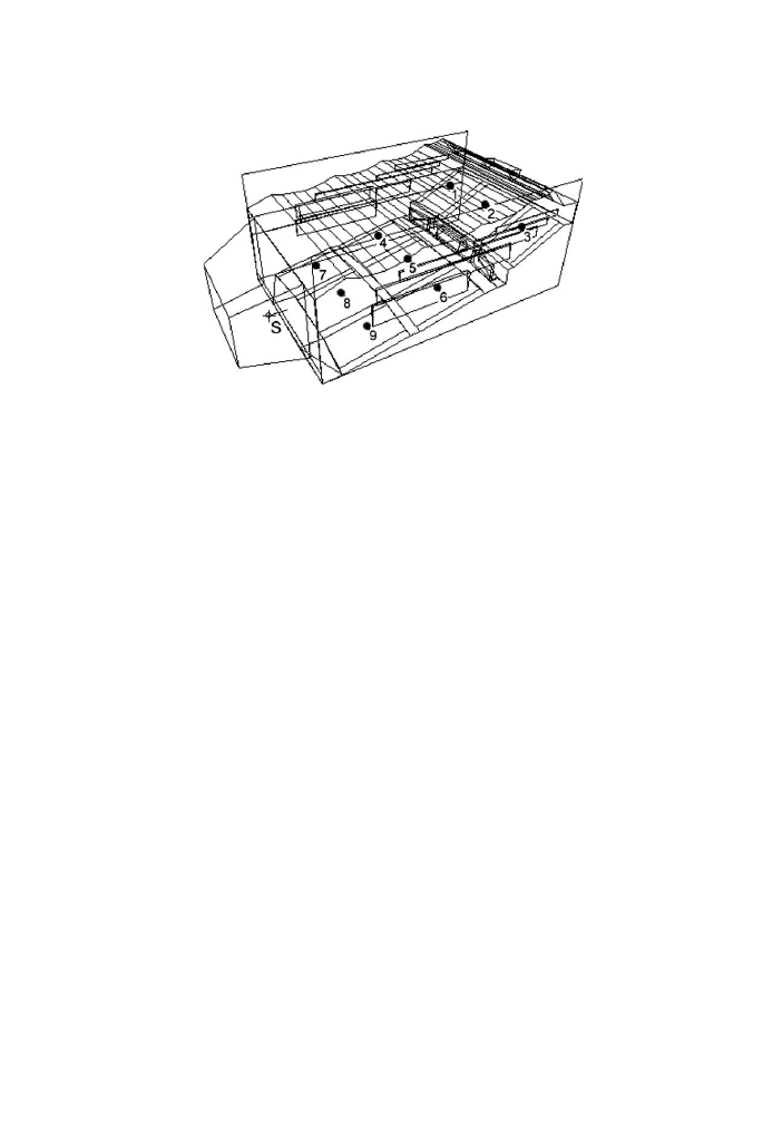
The modelled room is the Symphony Hall in the Conference Hall of Navarre, in

Pamplona, Spain

[11]

. This room is of rectangular shape with 1552 seats in two areas

separated by a balcony of 3 m. Such areas are inclined 10

° and 25° (see

Fig. 1

). Seats

are planned in three rows with middle and lateral aisles. The area of the stage is
520 m

2

(27.7 m wide and 18.8 m long) and the area for the audience is 1252 m

2

.

The pit has a capacity for 105 musicians. The total volume of the Symphony Hall
is 20,000 m

3

. When used as concert hall, an acoustic shell with a surface of 766 m

2

is

placed on the stage. The most common material is beech wood on the floor, walls
and acoustic shell. Whereas, the roof – which simulates four large sails – is made
of beech plywood.

2. Room acoustical simulation software – modelling work

Two commercial programs were used for the simulations. They will subsequently

be identified only by a number in order to preserve their anonymity as it is not the
purpose of this work to rate them. In addition, an objective rating of the software
should take into account many properties that may be of different importance to
the individual user: features of the construction and debugging of the room model,
tools for display and interpretation of the results, auralization facilities, feedback

Fig. 1. Sketch of concert hall, source and receiver positions.

R. San Martin, M. Arana / Applied Acoustics 67 (2006) 1–14

3

with developer, etc. All these aspects have to be borne in mind when a commercial
room simulation software is purchased. However, reliability of calculated results is
commonly regarded as the main criteria for the comparison. With the aim of consid-
ering the software as the only variable which could be responsible for the differences
in the calculation results, some considerations follow.

2.1. Simulation algorithms and modelling accuracy

Most of the required time to carry out a study of room acoustics by computer

simulation is spent on generating the geometric model. Experience in simulating
can result in a considerable reduction of the time used for the simulation of a room.
As a general rule, greater accuracy in the model will lead to greater precision in the
results obtained. However, it is very useful to know the characteristics of the pro-
gram. When it comes to carrying out a simulation, the most important concern is
to know the size of the surface areas in the room. Geometric acoustic laws consider
all the surfaces as infinite – in comparison with wavelengths – in the calculation of
the reflected energy. This limitation is considered differently by programs which con-
sider, for instance, diffraction algorithms, minimum size of the surface to be taken
into account, etc. An accurate simulation implies a great increase in the time used,
not only to draw the model, but also for the subsequent computer processing. The
balance between the processing time and the precision of the results is a matter
for the user to decide. Furthermore, it is neither possible nor necessary to model each
single edge in a concert hall to obtain correct results. In fact, an excessively high geo-
metrical resolution could even reduce the accuracy of the calculation.

P1 recommends a Ôreasonably largeÕ surface size for models to simulate. It intrin-

sically considers a surface size limit from which it introduces an algorithm that
approximates losses due to diffraction. This surface size limit is only applied to early
point source reflections. For this P1 recommends avoiding very small surfaces – re-
ferred to a dimension rather than an area – in those parts of the room contributing
strongly to first reflections. P2, on the other hand, does not consider any lower limit
for the size of the surfaces.

Both programs, however, make use of hybrid calculation methods, which com-

bine the best features of the image sources and ray-tracing methods. The main dif-
ference is that in P1, late reflections are calculated using a special ray tracing
process generating diffuse secondary sources. Every time a late ray is reflected on
a surface, a small secondary source is generated with a directivity according to Lam-
berts Law. This process does not produce exponentially growing number of reflec-
tions but keeps the same reflection density in all the calculations in order to keep
down calculation times.

With respect to the treatment of the diffusion there are slight differences between

each program. The diffusion coefficient of a surface is defined as the ratio between
reflected sound power in non-specular directions and total reflected sound power.
One weakness of the definition is that it does not say what form the directional dis-
tribution of the scattered power takes. Diffuse reflections are simulated by statistical
methods. In the method used by P1 the reflected direction of a ray is calculated as a

4

R. San Martin, M. Arana / Applied Acoustics 67 (2006) 1–14

weighted direction between the specular and the scattering direction, where a scatter-
ing coefficient of zero means that the scattered direction is not taken into account.
With scattering coefficients of one, the surface reflects the ray ideally scattered and
the reflected direction is calculated as a random direction following the angular Lam-
bert distribution of ideal scattered reflections. The method used in P2 to handle dif-
fusion is as follows: firstly, the specular parts of all the reflections are calculated
taking into account both the diffusion and the absorption coefficients. Secondly, each
time a ray hits a surface, a random number between 0 and 1 is generated. If the num-
ber is lower than the diffusion coefficient of the surface, a single ray is radiated in a
random direction. If the number is higher than the diffusion coefficient of the surface,
the ray is reflected in a specular direction. Since the diffusion coefficients are fre-
quency-dependent, a new ray-tracing process has to be started for each frequency
value.

The main consequence of these differences is that while the processing time is

approximately constant in P1, the corresponding time in P2 increases considerably
depending on the accuracy of the simulation.

Table 1

shows the comparison of

the processing times needed by programs using the same computer for five different
geometrical models with increasing number of surfaces. It has been decided to show
a processing time ratio because of the different times need by different computers.

2.2. Geometry modelling

For both programs, the graphic editors are complicated and of limited power.

They convert the geometrical data from CAD by using DXF format. No problems
were found with it. The stage was modelled with the acoustic shell placed on it. The
final room model was carried out with a total of 156 surfaces resulting in a mean free
path of 13.5 m. A non-directional source was located (simulated) at the centre of the
stage. A total of 9 receivers were located on the audience area, as is shown in

Fig. 1

.

2.3. Material properties

These programs make use of material libraries with data on absorption coeffi-

cients as well as common acoustic sources, with their power and directivity. Such li-
braries are similar and both can be edited and expanded. Differences of up to 10% in
absorption coefficients were found. More data on diffusion coefficients, though, are
required.

Table 1
Comparison of processing time versus number of surfaces

Model

Number of surfaces

Processing time ratio (P2/P1)

1

40

0.98

2

82

1.08

3

156

1.32

4

252

2.25

5

1497

4.72

R. San Martin, M. Arana / Applied Acoustics 67 (2006) 1–14

5

Except for the absorption coefficients of seats – measured following ISO 20354

Standard – the absorption and scattering coefficients of most surfaces were taken
from those libraries. However, one of the programs obliged us to use the same dif-
fusion coefficients for all frequencies. Previous research indicated that diffusion coef-
ficients of 0.1 and 0.7 were best suited for smooth and rough surfaces, respectively

[10]

. Definition of scattering parameters in the frequency domain would, neverthe-

less, improve predictive accuracy. It may be advantageous too, to weight diffusion
coefficients at low frequencies according to surface dimensions. Scattering due to
the finite size of a surface is most pronounced at low frequencies, whereas scattering
due to irregularities of the surface occurs at high frequencies. Finally, the ambient
conditions and the air absorption coefficients were taken into account due to the
great volume of the room. The values for calculations are shown in

Table 2

.

2.4. Calculation parameters

The calculation parameters were chosen taking into account previous studies and

the recommendations of each program. The length of the impulse response should be
similar to the reverberation time of the room and both programs allow it to be esti-
mated by means of a previous statistical analysis. The impulse response length was
2.5 s with a resolution of 10 ms. The number of rays was 50,000. The energy decay
curve, EDC, became stable at this number of rays. The reflection order was 65. Other
stop criterions (dynamic range, maximum travel time) were increased so that they
would not be an influence.

3. Measurements, results and discussion

Once the Hall was built, experimental results were obtained using the MLS tech-

nique following the standards requirements of ISO 3382. A dodecahedron source
was placed at the centre of the stage at a height of 1.5 m.

Table 3

shows the sound

power levels by octave bands of the source.

Obviously, identical levels had to be assigned to the acoustic source in the mod-

elling. It was intended to get an idea of the precision and limits of calculating the
acoustical properties of a concert hall in the planning stage. This was the only adjust-
ment with respect to previous simulations that was required in order to compare

Table 2
Absorption and scattering coefficients for materials and air absorption

1/1 (Hz)

63

125

250

500

1 k

2 k

4 k

8 k

Scatt.

Beech wood

0.25

0.25

0.34

0.18

0.10

0.10

0.10

0.10

0.1

Stairs

0.25

0.25

0.34

0.18

0.10

0.10

0.10

0.10

0.3

Glass

0.05

0.06

0.04

0.02

0.02

0.02

0.02

0.02

0.1

Chairs (unoccupied)

0.36

0.36

0.67

0.81

0.87

0.73

0.65

0.65

0.7

Air abs. (dB/100 m)

0.0

0.0

0.1

0.1

0.3

0.6

2.1

7.4

6

R. San Martin, M. Arana / Applied Acoustics 67 (2006) 1–14

sound pressure level, SPL and speech intelligibility index, STI. Results predicted by
the two software and measured for different parameters follow.

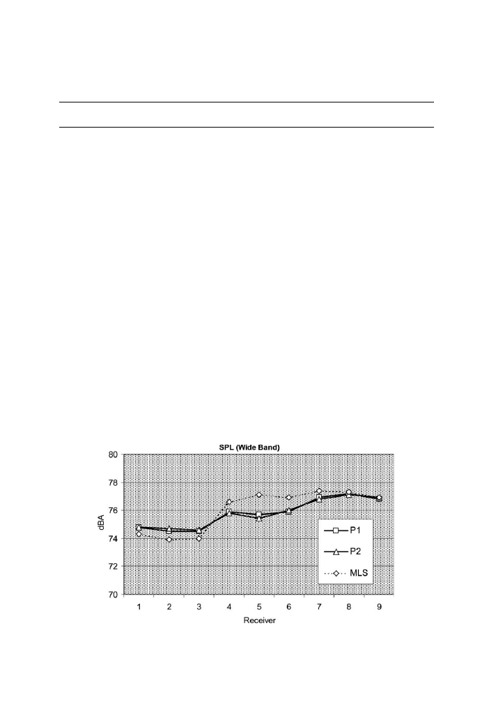
3.1. Sound distribution

Fig. 2

shows the SPL (Wide Band) calculated and measured at the 9 receiver posi-

tions. The calculated and measured SPL seems to be reasonably similar. When com-
paring the levels in different octave bands, SPL seems also to be reasonably similar
but larger differences are revealed at certain frequencies.

Fig. 3

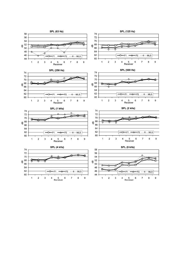
shows the results by

octave bands and by receiver points.

Differences between calculated and measured values in the 63 Hz octave band

show that for a more precise calculation of frequencies below 100 Hz other methods
should be applied in the software. The result for P1 and P2 in 8 kHz seems to be re-
lated to the air absorption coefficient in that frequency. The gap is higher when dis-
tance from source to receiver increases (see

Fig. 1

).

The differences found in the 125 Hz octave band between each program are more

difficult to explain. The wavelength in the 125 Hz octave ranges from 1.93 to 3.86 m
which may correspond to the distance between source and stage edge. Simulations
were carried out without taking into account diffraction edges because one of the
programs was unable to work with these. Another explanation could be the different
treatment of surface size limit mentioned above regarding reflections from the ceiling
and the way they have been modelled.

Table 3
Sound power levels by octave bands of the source

1/1 (Hz)

63

125

250

500

1 k

2 k

4 k

8 k

SPL (dB) (ref. 1 pW)

78.4

95.2

99.0

96.6

97.1

96.0

97.1

81.6

Fig. 2. Sound pressure level (dBA) calculated by the programs and measured at the 9 receiver positions.

R. San Martin, M. Arana / Applied Acoustics 67 (2006) 1–14

7

3.2. Reverberation times

Both reverberation time, T

30

, and the early decay time, EDT, at the 9 receiver

points are compared in

Figs. 4 and 5

. Calculated reverberation times were similar

in medium and high frequency bands. P1 gave results slightly greater than P2.
Differences of up to three times the just noticeable difference, jnd, for reverberation
times

[12]

were found in particular cases at low frequencies. Experimental results are,

in general, significantly higher than those predicted by programs. The deviations for
EDT predictions were also notably higher than for T

30

predictions. The accuracy of

Fig. 3. SPL in octave bands by receiver points.

8

R. San Martin, M. Arana / Applied Acoustics 67 (2006) 1–14

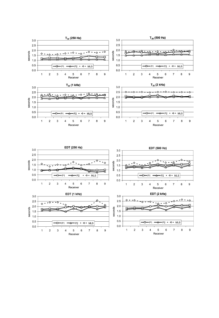
EDT is affected more by the modelling of early reflections. Also, its dependency on
the position of the receiver is also higher than the T

30

Õ

s, which is logical due to the

use of lower integration times in order to derive the parameter.

It is clear that the room is too brilliant. The brilliance index varies from 1.07 by

receiver 8 to 1.20 by receiver 1 (mean value: 1.15) evaluated from T

30

. The brilliance

index varies from 1.04 by receiver 7 to 1.15 by receiver 6 (mean value: 1.12) evaluated

Fig. 4. T

30

calculated by the two programs and measured at the 9 receiver points.

Fig. 5. EDT calculated by the two programs and measured at the 9 receiver points.

R. San Martin, M. Arana / Applied Acoustics 67 (2006) 1–14

9

from EDT. With regard to bass ratio index (warmth feeling) values are 0.81 from
EDT to 0.89 from T

30

. Obviously, Bass Ratio values are too small. Results evaluated

from reverberation times by P1 are, in general, higher than those evaluated by P2 at
low and medium frequencies.

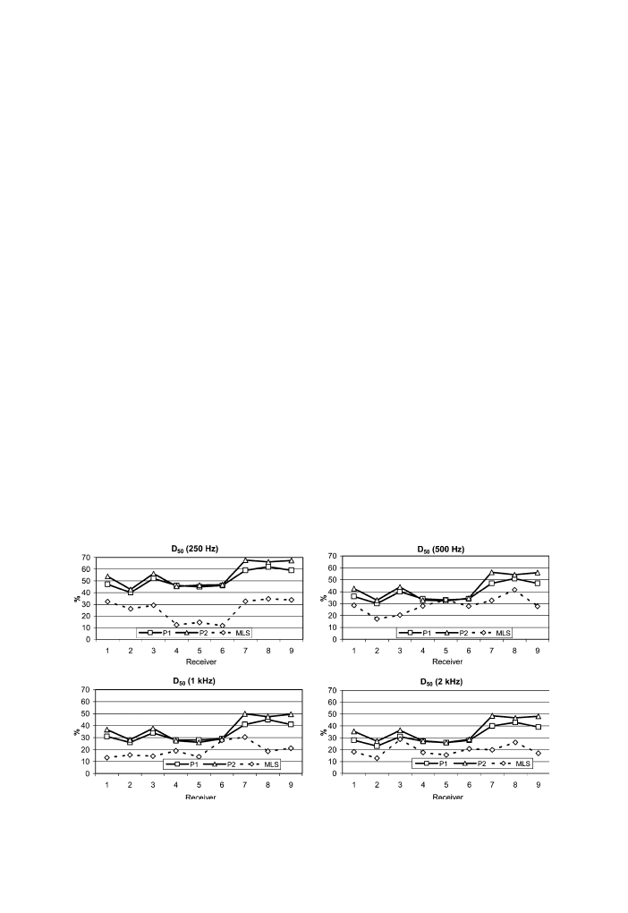
3.3. Balance between early and late arriving energy. Definition, D

50

, clarity, C

80

, and

centre time, Ts

Values for D

50

in the four central bands are shown in

Fig. 6

. Even though the

shape of the curves versus the receiver point is very similar for both programs, dif-
ferences with respect to the experimental results are significant in most cases. Higher
D

50

at the near receiver points (7, 8 and 9; see

Fig. 1

) due to the influence of the direct

sound is duly predicted by both programs. When comparing the calculated values of
each program, a difference of almost 2 jnd

[12,13]

(9% for D

50

and 1.9 dB for C

80

)

was found in receivers most distant to the source. P1 predicts greater values of
EDT than P2 as well as lower values of D

50

and C

80

. For linear decay of the impulse

response – in dB – this result has to be expected. The same comments are applicable
to the C

80

parameter.

On the other hand, differences between experimental and predicted values are very

high especially for low frequencies. This could be due to the influence of sound prop-
agation over seats which has not yet been implemented in room simulation software.
The seat dip effect is the name given to the problem of the selective low-frequency
attenuation of sound passing over seating at grazing incidence. Its primary cause
is interference between the direct sound travelling from the stage of an auditorium
and multiple reflections from the seating and floor. Seat dip attenuation has a

Fig. 6. Values of the definition, D

50

, for the four central bands.

10

R. San Martin, M. Arana / Applied Acoustics 67 (2006) 1–14

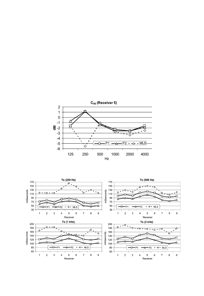
marked effect on parameters sensitive to the early energy field. Previous research

[14]

shows a decrease in C

80

of 5 dB from mid to low frequencies, and a corresponding

increase in Ts of 45 ms. In spite of not fulfilling the requirements on the angle of ele-
vation, some similar effect is taking place in the studied auditorium. Values for C

80

(125 Hz–4 kHz) are shown in

Fig. 7

at receiver 5.

Ts, normally given in ms, is the first moment of the impulse response.

Fig. 8

shows

the values of Ts, calculated and measured, for the four central bands. The general
time shift for the calculated Ts between P1 and P2 seems to be a systematic error
which may be due to an integration offset. Different statistical corrections for late
reflections may produce this effect too. Lower values for Ts in P2 are reflected in
higher calculated values in C

80

and D

50

, which enhances this line of argument. When

Fig. 8. Values of Ts for the four central bands.

Fig. 7. Values of the clarity, C

80

, for receiver 5.

R. San Martin, M. Arana / Applied Acoustics 67 (2006) 1–14

11

compared with measured values, it seems that the programs have under-estimated
the statistic tail correction of impulse response. This results in lower values of Ts
as well as higher values of D

50

and C

80

.

The size of the change at 250 Hz frequency band for Ts and C

80

, between mea-

sured and simulated values, is five times greater than the jnd for the same quantities
at mid frequencies. However, the threshold of perception of seat dip attenuation is
large enough to render low frequency C

80

values relatively unimportant

[15]

.

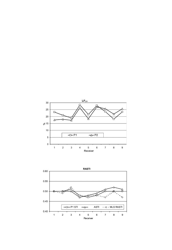
3.4. Lateral energy fraction

The lateral energy fraction, LF, is the ratio of the output of a

Fig. 8

microphone

(with its null direction aimed at the source and eliminating the direct sound) to the
output of a non-directional microphone. LF

E4

is the average LF in the four fre-

quency bands: 125, 250, 500 and 1000 Hz.

Fig. 9

shows the values of LF

E4

calculated

Fig. 9. LF

E4

calculated by the two programs at the 9 receiver points.

Fig. 10. Values predicted and measured for RASTI index at the 9 receiver positions.

12

R. San Martin, M. Arana / Applied Acoustics 67 (2006) 1–14

by the two programs at the 9 receiver points. Results evaluated by the two programs
are very similar and their dependence on the receiver point seems to be very logical
(see

Fig. 1

).

3.5. RASTI

A measured background noise level had to be introduced to the model in order to

achieve accurate evaluation of speech intelligibility. P1 evaluates the STI index but
not the RASTI. However,

Fig. 10

shows both the values predicted for such indices

at the 9 receiver positions and the RASTI values measured. No significant differences
were found between predicted and measured values.

4. Conclusion

Two room acoustical simulation software have been used to predict the main

acoustic parameters of a Symphony Hall. The calculation parameters were selected
by balancing the recommendations of the two programs. Even though the values
predicted by both software are very similar for some of the acoustic parameters
(SPL, LF

E4

, RASTI) there are notable differences in certain results, especially in

parameters derived from the impulse response (D

50

, C

80

and Ts) and in reverbera-

tion times. When comparing calculated values of SPL, differences of less than 0.5
dB were found in central frequency bands, with maximum differences of 2.5 dB
in 8 kHz as a result of a different air absorption coefficient in that frequency.
One program gave results slightly greater for reverberation times. Differences up
to 3 jnd were found in particular cases at low frequencies. With respect to energy
ratios, a difference of almost 2 jnd (9% for D

50

, 1.9 dB for C

80

and 19 ms for

Ts) was found in receivers furthest from the source. A general time gap for the cal-
culated Ts was found in all receivers and frequency bands. Different statistical cor-
rections for late reflections in each program seem to be the main reason for these
differences. The increased processing time of one of the programs, depending on
the accuracy of the simulation, is closely related to these differences in simulation
algorithms.

Experimental results were obtained using the MLS technique and compared with

calculated values. They show that the commercial programs largely coincide with
measured values and the dependence on position is to a great extent in line
with the measurements, although the limitation to geometrical acoustics still persists.
The difference between calculated and experimental results at the 63 Hz frequency
band was of up to 5 dB for SPL and 5 jnd for EDT. For reverberation times, exper-
imental results were, in general, slightly higher than those predicted by the programs.
These seem to have under-estimated the statistic tail correction of impulse response,
which results in greater values of D

50

and C

80

, and lower values of Ts. A more

exhaustive knowledge of scattering coefficients, including different treatment in the
frequency domain, may be a way of improving predictive accuracy. The influence
of sound propagation over seats has not yet been implemented in room simulation

R. San Martin, M. Arana / Applied Acoustics 67 (2006) 1–14

13

software. This may cause important differences between experimental and predicted
values for low frequencies.

Acknowledgements

The authors express their gratitude to the managers of the Baluarte Conference

Centre and Concert Hall of Navarre for their collaboration in providing the plans.
We also thank the Baluarte staff for their cooperation while measurements were
being taken.

References

[1] Rindel JH. Modelling in auditorium acoustic – from ripple tank and scale models to computer

simulations. Keynote Lecture. In: Forum acusticum. Seville, Spain; 2002.

[2] Krokstad A, Strom S, Sorsdal S. Calculating the acoustical room response by the use of a ray tracing

technique. J Sound Vibrat 1968;8(1):118–25.

[3] Vorla¨nder M. Simulation of the transient and steady-state sound propagation in rooms using a new

combined ray tracing/image-source algorithm. J Acoust Soc Am 1989;86:172–8.

[4] Rindel JH. The use of computer modeling in room acoustics. J Vibroeng 2000;3(4):41–72.
[5] Vorla¨nder M. International round robin on room acoustical computer simulation. In: Proceedings of

15th international congress on acoustics. Trondheim, Norway; 1995. p. 577–80.

[6] Bork I. A comparison of room simulation software –The 2nd round robin on room acoustical

computer simulation. Acustica – Acta Acust 2000;86:943–56.

[7] Bork I. Simulation and measurement of auditorium acoustics – the round robins on room acoustical

computer simulation. In: Proceedings of the institute of acoustics; 2002, vol. 24, Part 4.

[8] Yokota T, Sakamoto S, Tachibana H, Ikeda M, Takahashi K, Otsuru T. Comparison of room

impulse response calculated by the simulation methods based on geometrical acoustics and wave
acoustics. In: Proceedings of 18th international congress on acoustics. Kyoto, Japan; 2004.

[9] Gomes MHA, Gerges SNY, Tenenbaum RA. On the accuracy of the assessment of room acoustics

parameters using MLS techniques and numerical simulations. Acustica – Acta Acust 2000;86:891–5.

[10] Howarth MJ, Lam YW. An assessment of the accuracy of a hybrid room acoustics model with surface

diffusion facility. Appl Acoust 2000;60:237–51.

[11] San Martin R, Vela A, San Martin ML, Arana M. Comparative analysis of two acoustic simulation

software. In: Proceedings of forum acusticum. Seville, Spain; 2002. ARC-Gen-002.

[12] Cox TJ, Davies WJ, Lam YW. The sensitivity of listeners to early sound field changes in auditoria.

Acustica 1993;79:27–41.

[13] Bradley JS, Reich R, Norcross SG. A just noticeable difference in C50 for speech. Appl Acoust

1999;58:99–108.

[14] Davies WJ, Lam YW. New attributes of seat dip attenuation. Appl Acoust 1994;41:1–23.
[15] Davies WJ, Cox TJ, Lam YW. Subjective perception of seat dip attenuation. Acustica

1996;82:784–92.

14

R. San Martin, M. Arana / Applied Acoustics 67 (2006) 1–14