Models of Active Worm Defenses

David M. Nicol

Michael Liljenstam

Coordinated Science Laboratory

University of Illinois at Urbana-Champaign

Urbana, IL 61801

{nicol,mili}@crhc.uiuc.edu

ABSTRACT

The recent proliferation of Internet worms has raised ques-
tions about defensive measures. To date most techniques
proposed are passive, in-so-far as they attempt to block or
slow a worm, or detect and filter it. Active defenses take
the battle to the worm—trying to eliminate or isolate in-
fected hosts, and/or automatically and actively patch sus-
ceptible but as-yet-uninfected hosts, without the knowledge
of the host’s owner. The concept of active defenses raises
important legal and ethical questions that may have inhib-
ited consideration for general use in the Internet. However,
active defense may have immediate application when con-
fined to dedicated networks owned by an enterprise or gov-
ernment agency. In this paper we model the behavior and
effectiveness of different active worm defenses. Using a dis-
crete stochastic model we prove that these approaches can
be strongly ordered in terms of their worm-fighting capabil-
ity. Using a continuous model we consider effectiveness in
terms of the number of hosts that are protected from infec-
tion, the total network bandwidth consumed by the worms
and the defenses, and the peak scanning rate the network
endures while the worms and defenses battle. We develop
optimality results, and quantitative bounds on defense per-
formance. Our work lays a mathematical foundation for
further work in analysis of active worm defense.

1.

INTRODUCTION

A computer worm is so called because it has a life of

its own. Once burrowed into a susceptible system, it at-
tempts to propagate through the network. The usual means
is through “scans”, it attempts to connect to and infiltrate
other hosts throughout the network. Worms interfere with
normal use of computers, and exact an economic cost of
eradicating them and repairing systems infected by them.
Worms have the potential to wreak havoc on the systems
they infect, and on the networks they traverse. This poten-
tial has been realized already, several times.

The large-scale worm infestations in recent years have

Presented 2004 IPSI Conference, Studenica, Serbia, June 3-6 2004. This
research was supported in part by DARPA Contract N66001-96-C-8530,
NSF Grant CCR-0209144. In addition this project was supported under
Award No. 2000-DT-CX-K001 from the Office for Domestic Preparedness,
U.S. Department of Homeland Security. Points of view in this document are
those of the author(s) and do not necessarily represent the official position
of the U.S. Department of Homeland Security.

triggered several efforts to model worm spread in order to
understand how the low-level factors in the propagation
mechanism translate into macroscopic behavior, assess threat
levels of different worms, and evaluate the effectiveness of
detection methods and proposed counter-measures. Stan-
iford appears to have been the first to recognize that the
macroscopic propagation of the Code Red v2 worm could be
well modeled through the logistic equation [9]. This model
and the equivalent simple epidemic model from the epidemic
modeling literature (see e.g. [3]) have since been used in sev-
eral studies [10, 6, 7, 5, 12, 13]. [11] proposed a model to
take removals into account (based on the general epidemic
model ) and [1] proposed a discrete time model.

Our work is unique in considering a wide space of defensive

capabilities, and in sample path comparison of them. It is
most similar in spirit to [7, 1, 13] as we use epidemic models
to evaluate proposed worm counter-measures. We extend
simple epidemic models to consider the interaction of worms
and counter-worms and other “active” counter-measures.

For the purpose of illustration the experimental portion

of our paper uses parameters reflective of the Code Red v2
worm, released in July 2001. It is important to remember
that as far as the mathematics goes, time-scale is irrelevant.
Having said that, it is true that very fast worms have had
their propagation shaped by the impact they have on the
network infrastructure, and the simple mathematical models
we develop would not apply.

We focus on worms that spread autonomously by probing

other systems for vulnerabilities that can be exploited to
propagate from one machine to another. This class of worms
captures the essence of the rapidly spreading large-scale in-
festations seen to date, such as Code Red v2, Code Red
II, and Nimda in 2001, and Slammer, Blaster, and Welchia
in 2003. Thus, we deliberately exclude most typical email
born viruses that require a user action to enable infection.
In contrast, worms such as Slammer have proven that the
time-scales involved for fast moving autonomously propa-
gating worms can be so short that human intervention to
stop them is impossible. Consequently, this class of worms
poses a substantial threat and a trigger for development of
automated defensive mechanisms, such as those we consider
in this paper.

In the wake of one worm attack (Blaster), a counter-

worm (Welchia) was launched that sought hosts infected by
Blaster, attempted to patch them, and use them to find
other infected hosts. Whatever the intentions of the au-
thors might have been, Welchia had consequences as bad or
worse than Blaster—it was harder to get rid of, and effec-

tively created a denial-of-service attack on patch servers, so
that people trying manually to protect their systems had a
harder time doing so. The question is raised therefore of
the effectiveness and impact that an “active defense” might
have. We examine this question agnostically and without
overt consideration of the legal and ethical issues raised by
wide-spread active defense. It is enough for us that an or-
ganization as large as the United States Department of De-
fense could mandate such measures on its own gargantuan
networks; we seek to understand the power and the limita-
tions of active defense deployment, should they be deployed.
Our approach is analytic. We consider four aspects of active
defense—patching uninfected hosts, increasing the active de-
fense population by using uninfected hosts that are suscep-
tible to the worm, suppression of infected hosts discovered
through scans, and suppression of infected hosts discovered
through scans and traffic analysis. Using a very general dis-
crete stochastic model, we show that adding each capability
(in that order) to the active defense assumptions results in a
stochastically stronger increase in worm-fighting power. Us-
ing a continuous model we quantify some aspects of active
defense behavior, and prove some results about it.

2.

ACTIVE DEFENSE

Imagine a network where there are N hosts with a par-

ticular set of vulnerabilities, and then a worm is released
that is able to exploit one or more of these. We suppose
that a host infected by this worm scans the network look-
ing for vulnerable hosts it may infect. We assume that a
scan consists of a random selection of an IP address— if
that host is susceptible and uninfected it immediately be-
comes infected. In our discrete model we assume that the
address selection is oblivious to the state of the network.
This means that non-uniform random scanning can be ac-
commodated in the model, so long as the sampling is not
affected by any knowledge of other hosts, infected or not.
This does not preclude the sort of stratified sampling seen
in some worms (where hosts “closer” to the infected one are
sampled with higher probability), but it does preclude a dy-
namic partitioning of the search space based on coordination
among infected hosts. We assume a random delay of time
between successive scans from a host, once again assuming
that the sampling is independent of network state.

Under these assumptions we can picture the behavior of a

worm on a time-line populated with scan events. Each scan
event has a source and destination identity. Each of the sus-
ceptible hosts has a state of uninfected, or infected. A scan
event that has an uninfected host as destination changes
that host’s state, and thereafter it contributes to the scan-
ning. (It is straightforward to augment the model to account
for latency between when a scan is sent and when it is re-
ceived, we have not done so for simplicity of exposition).

2.1

Defense Capabilities

At time 0 the worm is launched from w

0

of the N suscep-

tible hosts. Each infected host scans the network using a
randomized strategy that is oblivious to the network state.
We assume that the worm immediately inhibits further pen-
etration through the same vulnerability, but that a counter-
worm scanning it can recognize the presence of the worm,
(e.g. through observation of banner information that the
host’s software returns, revealing a version and build that
admits penetration through the known vulnerability).

We envision a model of active defense as follows. At time

T

0

> 0, some I

0

hosts begin executing an active defense.

Each of those hosts scans, using a strategy (probably, but
not necessarily random) that is oblivious to the network
state. Whenever one of these scans targets a susceptible
but uninfected host, that host becomes (instantly!) patched
to prevent infection from the worm. We call this a simple
patch defense. This defense (and all the others we consider)
presumes that the defensive mechanism was prepared be-
fore the worm was launched. So-called 0-day attacks, ones
that exploit previously unknown exploits, are fairly rare.
The vulnerabilities that worms exploit are more typically
announced when discovered, often with patches available.
More often than not the patch code reveals details worm
writers use to target as-yet unpatched systems. It is not un-
reasonable to suppose then that patching defense code could
be crafted along with the patch. A reason for not releasing
the patching defense in anticipation of a worm is that the
release would contain the code to exploit the vulnerability,
with no work or further cleverness needed by a worm-writer.
A patching defense must be coupled with a worm-detection
mechanism, such as those proposed in [5, 12].

One could increase the presence of the active defense by in-

creasing the number of hosts running the patching logic. So
we define a spreading patch defense as one where, when an
uninfected susceptible host is scanned, it is endowed with a
counter-worm that both patches, and scans. While the num-
ber of patching hosts remains constant in a simple patching
defense, it grows in a spreading patch defense. Such a mech-
anism has been seen in the wild [4].

A third presumed defensive capability is worm suppres-

sion. Suppose that when a patching host scans an infected
host it is able to identify the host as infected, and to suppress
the infecting scans from being seen elsewhere, thereafter—
it is able to nullify the infected host. For example, the
spreading-patch worm might have an ability to cause the in-
fection traffic to be filtered by a nearby router; another way
might be if every machine in an organization had a “lock”,
such that when the proper “key” is applied, some or all of
that machine’s external communication is inhibited—an or-
ganization’s active defense posture would include selective
suppression of machines thought to be infected. For our
purposes, the important thing is that the infected host be
discovered by a scan, and that thereafter it is no longer a
source of infection. We call this a nullifying defense.

A fourth presumed defensive capability takes advantage

of the fact that some attacks are complex enough to re-
quire that the attacking host use its legitimate IP address
as source in its packets (and we may anticipate that in the fu-
ture the ability to spoof source addresses will become much
diminished, through more active router verification proce-
dures). Because of this, a patching host that receives a scan
from an infected host could turn around and nullify the in-
fection. In this sniper defense one expects that infected
hosts diminish in number faster than when they are discov-
ered merely by scans.

2.2

Metrics

There are different ways of assessing an active defense.

When host integrity is paramount, then an appropriate met-
ric is the number of hosts infected by the worm. We define
I(D, t) to be the cumulative number of hosts infected by
time t under defense D. This metric is a random variables;

we will say that D

i

is more powerful than D

j

if for all t > 0

and n > 0,

Pr{I(D

i

, t) > n} ≤ Pr{I(D

j

, t) > n}.

When this relationship holds we say that the distribution
(with respect to randomness due to sampling) of I(D

j

, t)

is stochastically larger than I(D

i

, t)[8], denoted I(D

j

, t) ≥

st

I(D

i

, t). D

i

is more powerful in the sense that it does a

better job at preventing susceptible hosts from becoming in-
fected. This stochastic ordering is strong in its implications.
It is known that if X ≥

st

Y and f is any increasing func-

tion, then E[f (X)] ≥ E[f (Y )]. This has bearing then for
any system metric that depends monotonically on infection
counts, e.g., the probability of system failure would likely be
monotone increasing in the number of infected hosts.

An active defense may increase the overall scanning ac-

tivity on the network, and there is evidence that intense
scanning can harm the network [2]. When network health
is the principle concern, then measures of scanning history,
and/or scanning intensity are appropriate. If λ(D, t) de-
notes the scanning rate due to both worm and defense D,
then we assess a defense in terms of its peak scanning rates
over some interval [0, t]:

max

0<s<t

{λ(D, s)}

We might also assess it through its aggregate scanning rates
(the space-time product) over some interval [0, t]:

Z

t

0

λ(D, s) ds.

3.

ORDERING OF DEFENSES

Intuition suggests that the four active defensives (five, if

we include the empty defense) we’ve outlined might be or-
dered in terms of power. We now show that this is exactly
the case. In the comparisons made, we use the Common
Sample Path assumption, that once a host is infected (or
takes on the counter-worm), its scanning behavior is com-
pletely determined by a random number stream that is in-
dependent of any other. When we compare two defenses, we
assume that a host uses that same stream in both systems,
which allows us to compare the two systems on commonly
constructed sample paths. The implication is that once a
host is infected (or starts to run a counter-worm), its se-
quence of inter-scan delays are the same in both systems,
and the pattern of hosts scanned are the same in both sys-
tems. Thus, if the two systems cause a host to be infected at
the same instant, on the sample paths being compared that
host will scan exactly the hosts at exactly the same time, in
both systems.

The results to follow are based on a construction we call

the Sample Path Graph (SPG). For every susceptible host
h

i

let I

i

be a sequence of pairs (t

i

, dst

i

) identifying the time

since the host started infection scanning, and a destination
dst

i

of a scan. I

i

is ordered by increasing values of t

i

. We de-

fine C

i

similarly, describing the scanning pattern once a host

starts running a counter-worm. We construct a graph whose
nodes represent hosts that are assumed to be infected al-
ready at time 0 (and which have scanning sequences), nodes
representing hosts that eventually start counter-worm scans
(with their own scanning sequences), and susceptible hosts.
The graph contains a directed edge for every potential scan

described in the sets {I

i

} and {C

i

} whose target was suscep-

tible at time 0. The edge is directed from the source of the
scan to the target; an edge will be called an infection edge
or countering edge, depending on whether it comes from an
infection or counter-worm sequence, respectively. The node
for host h

i

will have values S(h

i

) recording the earliest time

it was scanned by an infected host, and C(h

i

) recording the

earliest time it was scanned by a host running a counter-
worm. Some of the edges are labeled with the time of the
scan—these edges are particularly important in our analy-
sis. The values of S(h

i

) and C(h

i

), the edges labeled and

the values of those labels all depend on the particular de-
fense. However, common to those defenses are the following
rules:

• All hosts assumed to be already infected at time 0 label

each of their edges with the corresponding scan time;

• all hosts that are used to start the counter-worm label

each of their edges with T

0

plus the corresponding scan

time offset contained in the scan sequence.

The differences between different defense’s SPGs are char-

acterized as follows:

Empty Defense (D

0

)

1. The node for host h

i

defines S(h

i

) to be the smallest

label among all labeled infection edges directed to it;
S(h

i

) = ∞ if no such edge exists.

2. A host h

i

labels the infection edge corresponding to the

j

th

element of I

i

(say, (s

j

, dst

j

)) with value S(h

i

)+s

j

,

j = 1, 2, · · · .

The difference between the simple patch defense and the

empty defense is that susceptible hosts are protected from
infection if they are touched by a countering scan before
being touched by an infection scan.

Simple Patch (D

1

)

1. Item (1) from the Empty Defense rules.

2. The node for host h

i

defines C(h

i

) to be the smallest

label among all labeled countering edges directed to it;
C(h

i

) = ∞ if no such edge exists.

3. If S(h

i

) < C(h

i

) the node labels the infection edge

corresponding to the j

th

element of I

i

(say, (s

j

, dst

j

))

with value S(h

i

) + s

j

, j = 1, 2, · · · .

4. If C(h

i

) < S(h

i

) the node does not label any of its

edges.

The difference between a spreading patch defense and a

simple patch one is that a host that receives a countering
scan before any infection scan becomes host to counter-worm
software, and generates its own countering scans.

Spreading Patch (D

2

)

1. Items (1) from the Empty Defense rules, (2), and (3)

from the Simple Patch rules.

2. If C(h

i

) < S(h

i

) the node labels the countering edge

corresponding to the j

th

element of C

i

(say, (s

j

, dst

j

))

with value C(h

i

) + s

j

, j = 1, 2, · · · .

The difference between a nullifying defense and a spread-

ing patch defense is that when a countering scan reaches a
host that is already sending infection scans, the infection
scans stop.

Nullifying Defense (D

3

)

1. Item (1) from the Empty Defense rules, item (2) from

the Simple Patch rules, and item (2) from the spread-
ing patch rules.

2. If S(h

i

) < C(h

i

) the node labels the infection edge

corresponding to the j

th

element of C

i

(say, (s

j

, dst

j

))

with value C(h

i

) + s

j

, for all j such that S(h

i

) + s

j

≤

C(h

i

).

And finally, the difference between a sniper defense and

a nullifying defense is that infection scans that encounter
hosts running countering scans cause the host sending the
infection scan to cease. This may occur before the host
is itself scanned by a countering scan (which has the same
nullifying effect).

Sniper Defense (D

4

)

1. Item (1) from Empty Defense rules, item (2) from the

Simple Patch rules, item (2) from the Spreading Patch
rules.

2. If S(h

i

) < C(h

i

), let k be the smallest index for (s

k

, dst

k

) ∈

I

i

such that S(h

i

) + s

k

> C(dst

k

), and define K

i

=

S(h

i

) + s

k

. The node for h

i

labels the infection edge

corresponding to the j

th

element of C

i

(say, (s

j

, dst

j

))

with value C(h

i

) + s

j

, for all j such that S(h

i

) + s

j

≤

min{C(h

i

), K

i

}.

The construction above make the conditions under which

a given infection edge is labeled increasingly restrictive, as
we move through sequence of defenses. This implies that if
we choose a host h

i

and defenses D

a

and D

b

with a < b,

then the set of labeled incoming infection edges it has in
the SPG for D

b

is a subset of the labeled incoming infection

edges it has in the SPG for D

a

. This fact enables us to prove

the central results comparing different defenses.

Lemma

1. Consider two defenses D

a

and D

b

, a < b, un-

der identical boundary conditions. Let G

a

and G

b

be corre-

sponding Sample Path Graphs constructed under the Com-
mon Sample Path assumption, and let S

(y)

(h) and C

(y)

(h)

denote the S(h) and C(h) variables for host h under de-
fense y ∈ {a, b}. Then for every host h, S

(a)

(h) ≤ S

(b)

(h)

and C

(b)

(h) ≤ C

(a)

(h).

Proof:

Without loss of generality renumber the hosts by

increasing value of S

(b)

(h), we induct on this order. Con-

sider the base case of h

0

. Both S

(a)

(h

0

) and S

(b)

(h

0

) are

defined by edges from hosts assumed to be infected at time
0, and are thus identical. In both G

a

and G

b

host h

0

gets

the same set of labeled countering edges from the initial
set of hosts running the defense, and C(h

0

) in both graphs

is no larger than the smallest of these labels. However, in
G

b

there may be more countering edges labeled, and hence

the possibility of a shorter path to h

0

through those edges,

whence C

(b)

(h

0

) ≤ C

(a)

(h

0

) and the induction base is es-

tablished. For the induction hypothesis we assume that the

assertion is true for all hosts h

0

, h

1

, . . . , h

n−

1

for some n,

and consider host h

n

. Let e be the labeled infection edge

coming into h

n

whose label defines S

(b)

(h

n

), and consider

its manifestation e

0

in G

a

. By the construction of SPG’s,

an infection edge may appear labeled in the SPG of one de-
fense D

u

and not another D

v

if its target h

y

has a smaller

value C(h

y

) in G

v

than in G

u

, or if G

v

is nullifying and

scans a countering host. In all cases the only way a labeled
edge appears in G

u

and not G

v

is when u < v. Conse-

quently e

0

appears labeled in G

a

. This in turn implies that

the node h

m

from which e

0

is directed satisfies m < n, as it

is directed from the same node in both G

a

and G

b

. By the

induction hypothesis S

(a)

(h

m

) ≤ S

(b)

(h

m

), which implies

that the label on e

0

is no larger than the label on e, and

thus, that S

(a)

(h

n

) ≤ S

(b)

(h

n

). A similar argument shows

that the labeled countering edge g which defines C

(a)

(h

n

)

(when this exists) has a labeled counter-part g

0

in C

(b)

(h

n

),

whose label is no larger in G

b

than it is in G

a

, and thus that

C

(b)

(h

n

) ≤ C

(a)

(h

n

). This completes the induction.

2

From this result comes the main result.

Theorem

2. For defense D

i

and every time t, let I(D

i

, t)

denote the number of hosts infected by time t (including
those that later become nullified). Then for a < b, I(D

a

, t) ≥

st

I(D

b

, t) for every t ≥ 0.

Proof: Lemma 1 shows that for any sample path of scans
and every time t, the number of hosts h with S

(a)

(h) ≤

t is greater than or equal to the number of hosts h with
S

(b)

(h) ≤ t. For any sample path these counts define the

random variables I(D

a

, t) and I(D

b

, t). Coupling results in

[8] establish the result.

2.

These results show that the difference between defenses is

structural, and strong. The results are very general, free of
distributional assumptions other than independent of sam-
pling from network state. However, they don’t give much
insight into how well these defenses perform.

There is one exception, in the special case where the counter-

worm has the same scanning characteristics as the worm.
Then we may assume that whenever a host is entered either
by a worm, or a counter-worm, its pattern of scans (inter-
scan delays, sequence of targets scanned) is the same under
any defense. From the point of view of the same path analy-
sis we’ve done, it means that whenever a node is triggered to
scan we may assume it does so with exactly the same pattern
regardless of if that is an infection or countering scan. This
means that any host that scans in an empty defense also
does so in a spreading patch defense, only possibly earlier
(if the scan is a countering scan).

These observations establishes the theorem.

Theorem

3. Suppose that the scanning structure of the

counter-worm is identical to the worm. For every time t
let λ(D

0

, t) and λ(D

2

, t) denote the instantaneous number

of hosts scanning under the empty defense and spreading
patch defense, respectively. Then for every t, λ(D

2

, t) ≥

st

λ(D

0

, t).

This theorem is a strong statement about a condition when
adding defense is worse, from the point of view of the net-
work. Increasing functions of λ(D, t) include the peak num-
ber of hosts scanning over an interval, the space-time prod-
uct of the bandwidth devoted to scanning, the probability
of network partition, and so on. The stochastic ordering as-
serts that the expectation of each of these is larger when we

use a spreading patch defense than when we use no defense
at all.

4.

EPIDEMIC MODELS

We use a style of modeling based on well known models

from the epidemic modeling literature. In typical simple
epidemic models we consider a fixed population of N , where
each individual is susceptible to infection, and each individ-
ual will, at any given time, be in one of a small set of prede-
fined states. For instance, in the simple epidemic model [3]
(aka the SI model and equivalent to the logistic equation)
an individual is either in state S (susceptible to infection)
or I (infected). We denote by s(t) and i(t) the number of
individuals in state S and I respectively at time t, and thus
∀t, s(t) + i(t) = N. For large enough populations, the mean
rate of state changes S → I can be modeled as:

ds(t)

dt

=

−βs(t)i(t)

di(t)

dt

=

βs(t)i(t)

where the constant β is the infection parameter, i.e. the
pairwise rate of infection. β reflects the aggregate scanning
rate of an infected host, as well as the mean probability of
selecting a given address for an individual probe attempt.
The system boundary conditions are given by the number
of initially susceptible hosts s(0) and initially infected hosts
i(0). This model rests on assumptions of homogeneous mix-
ing, which correspond well to a uniformly random scanning
worm spreading freely through a network, so in the follow-
ing we will refer to this the Random Scanning Worm
Model.

Other scanning strategies are possible. For instance, worms

such as Code Red II, Nimda, Blaster, and Welchia uti-
lized preferential (rather than uniform) scanning techniques
where addresses close in the address space to the scanning
host’s would be probed with higher probability. Other sug-
gested possibilities include a “Divide-and-Conquer” approach
to probing the address space (see “partitioned permutation
scan” in [10]). Here each worm is assigned a disjoint fraction
of the address space to probe.

Other simple tricks for speeding up the propagation have

been suggested, such as the use of pre-compiled hit-lists or
using inter-domain routing tables to only scan routed space
[13]. We can incorporate these into our framework; hit-listed
hosts can be made to be infected as a boundary condition,
and use of routing tables just increases β to reflect that the
scanning is over a smaller address space.

The early stage of infection is the most critical time for any

counter-measures to be effective. Since the worms behave
similarly in the early stages we will, in the following, focus
on random scanning worms as this is the type of worm that
has been observed in the wild to date.

In [7], Moore et al. note that when considering the effec-

tiveness of defensive measures, it is preferable to consider
the quantiles of infection rather than the mean number of
infections due to the variability inherent in the early stages
of infection growth. However, we prefer to use these mean-
value based models, because they lend themselves to analysis
in a way that stochastic simulations do not. Moreover, we
are mainly concerned with the relative performance of dif-
ferent defenses as we compare them, and we believe that the
relative performance can be credibly determined in terms of

the mean, even though the predicted mean absolute perfor-
mance should be viewed with caution.

4.1

Spreading Patch Counter-Worm

Consider the spreading patch counter-worm model dis-

cussed earlier, and assume that it uses the same vulnerabil-
ity and propagation strategy as the original worm. Under
these assumptions the second worm will spread at (approx-
imately) the same rate as the original worm, seeking the
same susceptible population of hosts. A simple model is:

ds(t)

dt

= −βs(t)(i

b

(t) + i

g

(t))

di

b

(t)

dt

= βs(t)i

b

(t)

di

g

(t)

dt

= βs(t)i

g

(t)

where i

b

refers to infections by the malicious (bad) worm

and i

g

refers to infections by the spreading-patch (good)

worm. Given β and i

b

(0), system behavior is governed by

the time T

0

at which spreading-patch worms are released,

and the number of worms I

0

released then. We assume

that the spreading-patch worms are launched on “friendly”
machines that are not part of the susceptible or infected set.

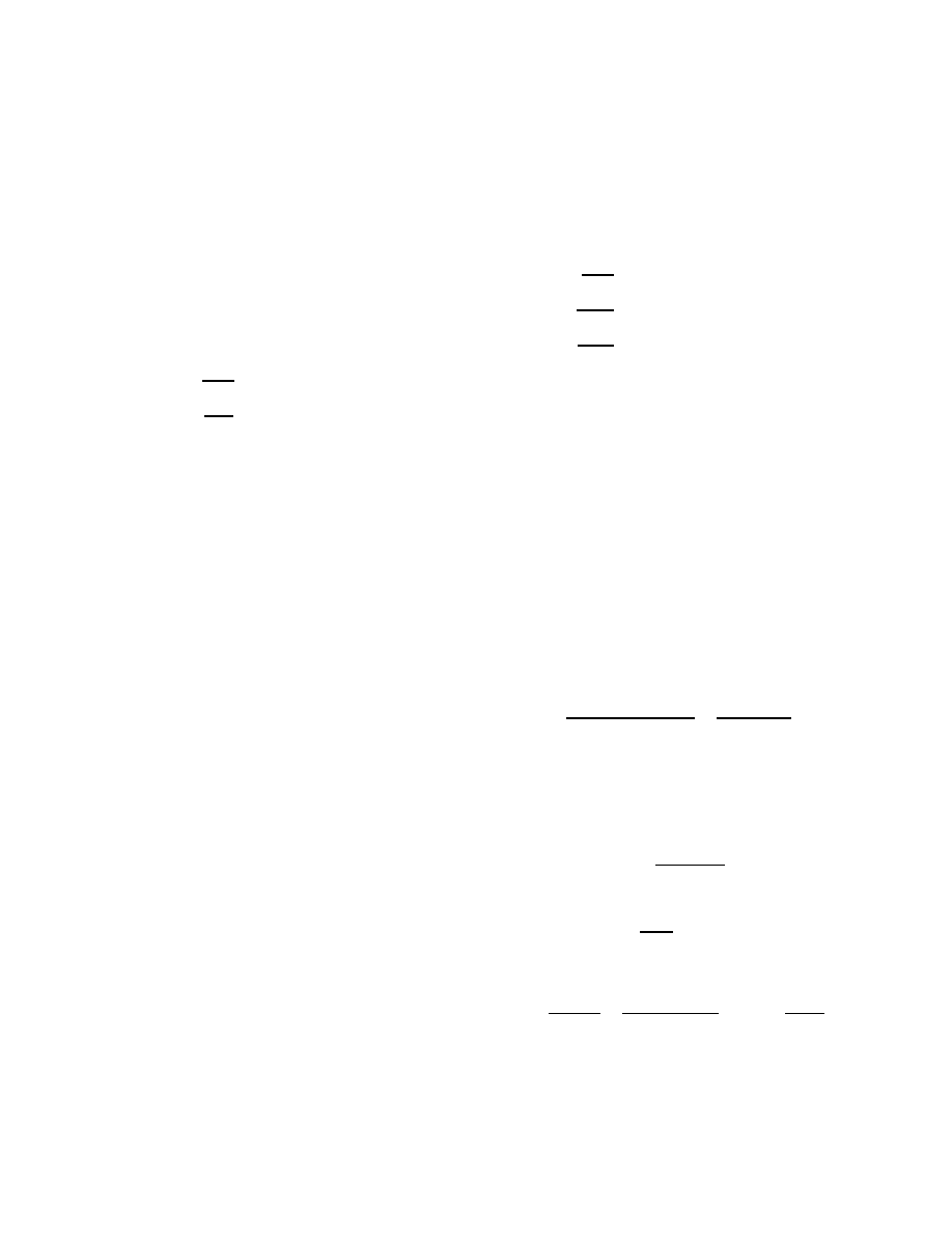
Spreading-patch worm effectiveness as a function of re-

sponse time and initial population is shown in Figure 1. An
effective response requires a combination of low response
time and a sufficiently large initial population. Launching
a single counter-worm has little effect, and the window of
opportunity for launching even a thousand spreading-patch
worms disappears after a couple of hours.

At T

0

, i

b

(T

0

) hosts have succumbed to the original worm

and there are s(T

0

) remaining susceptibles. How many

spreading-patch worms must be launched to protect a given
fraction fraction p of those remaining susceptibles? If we
consider the fraction of infection growth due to the spreading-
patch worm

di

g

(t)/dt

di

g

(t)/dt + di

b

(t)/dt

=

i

g

(t)

i

g

(t) + i

b

(t)

we see that since the propagation rates are the same, the
proportions of the susceptible population consumed by each
worm from T

0

onwards simply correspond to their propor-

tion of the population at T

0

. Thus, ultimately the fraction

of hosts which were susceptible at T

0

, but eventually are

patched is

p =

I

0

I

0

+ i

b

(T

0

)

.

Solving for I

0

we get

I

0

=

„

p

1 − p

«

· i

b

(T

0

)

(1)

Thus, the fraction of all susceptibles s(0) that will be pro-
tected is

˜

p =

p · s(T

0

)

s(0)

=

p[s(0) − i

b

(T

0

)]

s(0)

= p

„

1 −

i

b

(T

0

)

s(0)

«

If the infection is caught early on, then i

b

(T

0

) s(0), and

the protected fraction ˜

p ≈ p. Thus, equation (1) can be

used as a guideline for selecting I

0

given only an estimate of

how many hosts have been infected at the time of response
(i

b

(T

0

)), assuming that the response occurs early. Such an

0

200

400

600

800

1000

1

2

3

4

5

6

7

8

0

10

20

30

40

50

60

70

80

90

100

Response time (T

0

) [h]

Response Initial Population (I

0

)

% hosts infected by malicious worm

Figure 1: Effectiveness of spreading-patch worm as a function of response time and initial counter-worm
population.

estimate can reasonably be obtained by analysis of observed
scanning behavior.

The spreading-patch worm model considered here assumes

only that it scans at the same rate as the original worm. It
does not assume any information about the malicious worm
and its behavior. As worms to date have exploited vulner-
abilities that were previously known, it is not unreasonable
to suppose that a patching worm might be developed when
the vulnerability is identified (but before it is announced),
against the possibility of needing to use it. Such a worm
would not be launched before needed, because it could be
captured and analyzed for the means to exploit the vulner-
ability. However, the fact that the spreading-patch worm
has higher impact on the network (Theorem 3) than no de-
fense at all encourages us to explore counter-worms that
have stronger capabilities in worm identification and sup-
pression, with smaller impact on the network.

4.2

Nullifying Defense

Next we develop a continuous model of the nullifying de-

fense. Using notation similar to that for the spreading patch
defense, we develop state equations

ds(t)

dt

= −βs(t)(i

b

(t) + i

g

(t))

di

b

(t)

dt

= βs(t)i

b

(t) − βi

b

(t)i

g

(t)

di

g

(t)

dt

= βs(t)i

g

(t)

Here we see a new component to (di

b

(t)/dt), the subtraction

of hosts due to being scanned by the counter-worm.

Under our assumptions, in the limit of increasing time t,

the aggregate scan rate under the spreading patch defense

is proportional to the number of “outside” spreading-patch
hosts I

0

plus the initial susceptible population size s(0)—

eventually every susceptible host is running either the worm,
or the counter-worm. However, in the case of nullifying
worms, the aggregate peak scan rate may be smaller than
the aggregate peak scan rate of the unfettered worm.

Theorem

4. Suppose that I

0

initial nullifying worms are

released at time T

0

. If I

0

≤ i

b

(T

0

), then the aggregate peak

scan rate using the nullifying worm is less than the peak scan
rate of the unfettered worm.

Proof.

Let i

n

(t) be the aggregate number of infected

hosts that a nullifying defense has identified and contained
by time t, and let e(t) be the number of formerly suscep-
tible hosts that have been “enlisted” to run the nullifying
worm. At any time t the aggregate scan rate of a defense
is proportional to i

b

(t) + i

g

(t) = i

b

(t) + I

0

+ e(t). From the

invariant s(0) = s(t) + i

b

(t) + i

n

(t) + e(t) we replace e(t)

in the scan rate expression to see that the scan rate at t is
proportional to I

0

+ s(0) − s(t) − i

n

(t). The maximum value

of this term will always be less than s(0) if I

0

< s(t) + i

n

(t)

for all t. Examination of derivatives shows that s(t) + i

n

(t)

is monotone decreasing, hence its lowest value is the asymp-
totic value of i

n

(t), say, N = lim

t→∞

i

n

(t). By assumption

I

0

≤ i

b

(T

0

), and clearly i

b

(T

0

) < N . The conclusion follows

immediately.

It is interesting to compare this result—which says if one

limits the initial infection of the counter-worm you can bound
the peak scan rate from above, with the spreading-patch de-
fense results which turn these inequalities around. With the
spreading-patch defense a minimum size of the release needs
to be I

0

> i

b

(T

0

) to give it enough mass to overtake the

original worm. But because the nullifying worm fights by

decreasing the number of scanning worms, it gets by with a
smaller initial counter-worm population.

Another capability a nullifying defense could have is that

it stop all defensive scanning, upon centralized command.
This would help mitigate against overwhelming the network
with scans from the defenses (a characteristic reported of
the counter-worms seen in the wild). Denote the defensive
worm stopping time by t

s

. The modified state equations

after time t

s

are

ds(t)

dt

= −βs(t)i

b

(t)

(2)

di

b

(t)

dt

= βs(t)i

b

(t)

(3)

di

g

(t)

dt

= 0

(4)

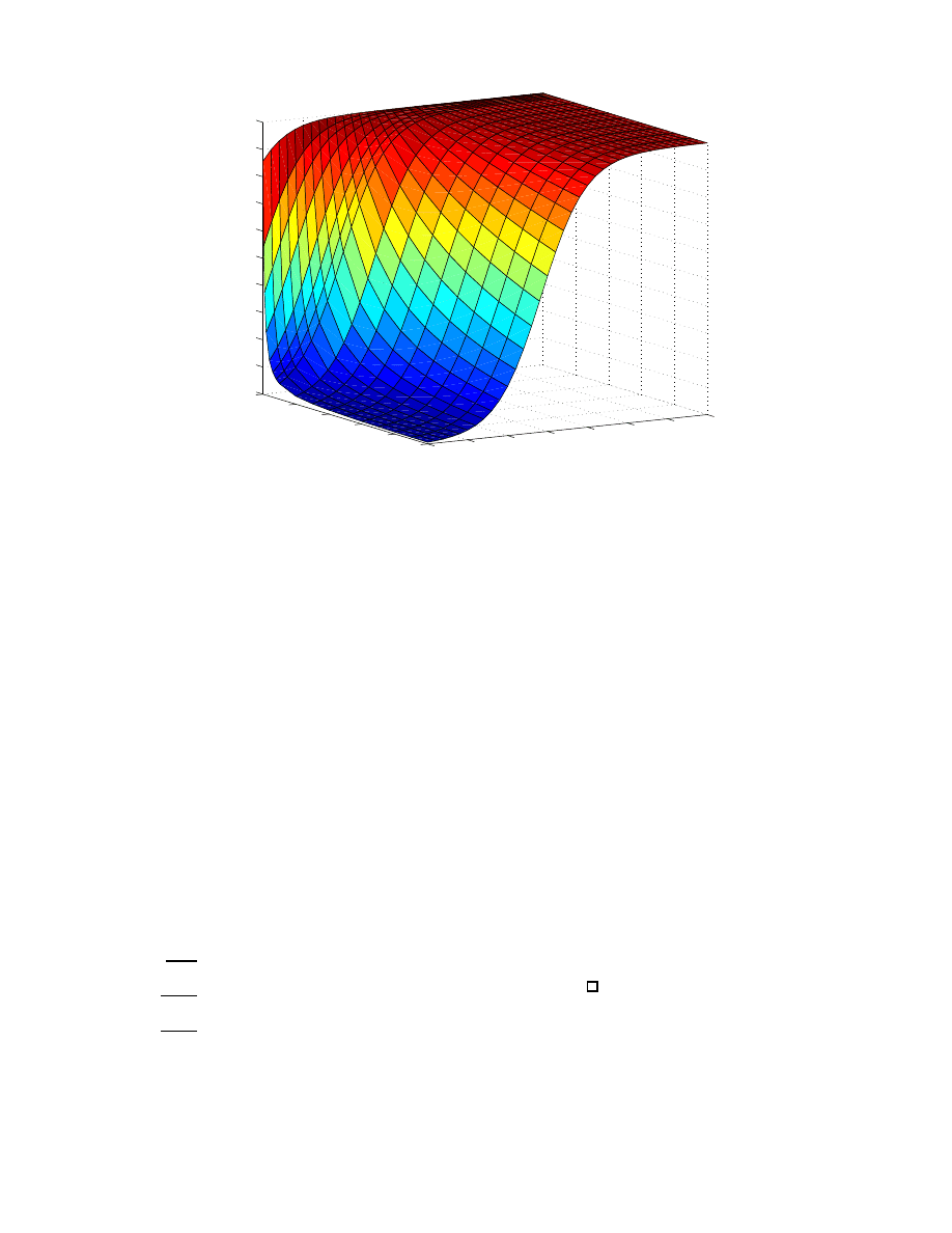
Figure 2 illustrates the evolution of system state where the
nullifying defense is propagating without stopping. Also
shown, is the resulting peak total population (directly re-
lated to peak bandwidth in our model) as a function of
stopping time t

s

. Taking the time at which the defensive

worms are stopped as a control parameter, we see that the
minimized peak scan rate obtained by optimally selecting
the stopping time is no larger than the peak scan rate if the
defenses are never turned off. This capability can only im-
prove the peak scan rate over that of the earlier nullifying
defense we considered.

For t < t

s

the scan rate is proportional to i

b

(t) + i

g

(t); the

peak scan rate achieved after t

s

is proportional to i

b

(t

s

) +

s(t

s

), for the original worm will eventually infect all hosts

left unprotected once we stop the defensive scans. Exami-
nation of derivatives shows that

d(i

b

(t) + i

g

(t))

dt

= β (i

b

(t)(s(t) − i

g

(t)) + s(t)i

g

(t))

which we observe is positive at least as long as s(t) ≥ i

g

(t).

Likewise, derivatives show that i

b

(t) + s(t) is a decreasing

function :

d(i

b

(t) + s(t))

dt

= −βi

g

(t)(i

b

(t) + s(t)).

If the nullifying defense scans are stopped at t

s

with s(t

s

) ≥

i

g

(t

s

) we are assured that the peak scanning rate of the sys-

tem is

max{i

b

(t

s

) + i

g

(t

s

), i

b

(t

s

) + s(t

s

)}.

So long as the first argument is increasing and the second
argument is decreasing, the stopping time that minimizes
the maximum occurs when the arguments are equal, e.g.,
when i

g

(t) = s(t); since i

b

(t) + i

g

(t) is still monotone at

this point, t

s

minimizing the peak aggregate scanning rate

satisfies i

g

(t

s

) = s(t

s

).

We are in a position now to quantify the performance of a

defensive worm. We can show that the minimal peak num-
ber of hosts scanning is at least (1/3)(s(0) + I

0

), provided

that I

0

≥ i

b

(T

0

), a result which we state formally.

Theorem

5. Consider a nullifying defense that is launched

at time T

0

with I

0

≥ i

b

(T

0

) initial instances, and whose

scans can be stopped on command. The stopping time t

s

which minimizes peak scanning is the unique solution to
i

g

(t

s

) = s(t

s

). A lower bound on the peak number of hosts

scanning is (1/3)(s(0) + I

0

).

Proof: We first note that under the assumption I

0

= i

g

(T

0

) >

i

b

(T

0

), that i

g

(t) ≥ i

b

(t) for all t ≥ T

0

. This is a result

of both the worm and the counter-worm competing for ex-
actly the same pool of susceptible hosts—at the same rate
(per host)—with the counter-worm starting with at least as
many hosts as are in the infection at the time the counter-
worm is released. A consequence is that the time t

s

when

s(t

s

) = i

g

(t

s

) occurs before the time t

b

that s(t

b

) = i

b

(t

b

).

This fact turns out to be important as we ask for condi-
tions under which i

g

(t) ≥ i

n

(t), where i

n

(t) is the number

of infected hosts that have been nullified. We know that
i

g

(T

0

) > i

n

(T

0

); analysis of the derivative of i

g

(t) − i

n

(t)

shows that this difference grows so long as s(t) ≥ i

b

(t)—a

condition which can only occur after the stopping time t

s

.

Finally, we note the invariant

i

b

(t) + i

g

(t) + i

n

(t) + s(t) = s(0) + I

0

.

At the stopping time, s(t

s

) = i

g

(t

s

), and i

g

(t

s

) > i

n

(t

s

),

whence

i

b

(t

s

) + 3i

g

(t

s

) > s(0) + I

0

.

It follows that i

b

(t

s

) + i

g

(t

s

) > (1/3)(s(0) + I

0

).

2

We see that the capabilities nullifying defensives have over

spreading-patch defenses (suppress an infected host’s scans,
stop the “good worm” scanning) serve to give it greater
power, but the peak number of hosts scanning (both worm
and counter-worm) is still at least one third of the initial
susceptible population. We push on looking for ways of
countering worms with increasing power, while reducing the
impact on the network.

4.3

Sniper Worm

We can increase the power of defense if we can use traffic

analysis to identify the source of infection scans, what we
have called “snipers” earlier in the paper. A sniper would
be a highly sophisticated worm that could nullify on con-
tact (by the counter-worm scanning) detect incoming worm
scans, and consequently nullify the originating source. In
this case any interaction between the bad and the good
worms lead to bad worm reduction, so our Sniper Worm
Model becomes:

ds(t)

dt

= −βs(t)(i

b

(t) + i

g

(t))

di

b

(t)

dt

= βi

b

(t)[s(t) − 2i

g

(t)]

di

g

(t)

dt

= βi

g

(t)s(t)

Coefficient ’2’ in the equations above reflect that a worm
becomes nullified when either it scans a counter-worm, or
vice-versa.

Like the simpler nullifying defense models, we may switch

off the counter-worm scanning, say at time t

s

. Under these

assumptions, for points in time after the counter-worm stops
scanning, the sniper worm equations become

ds(t)

dt

= −βs(t)i

b

(t)

di

b

(t)

dt

= βi

b

(t)[s(t) − i

g

(t

s

)]

di

g

(t)

dt

= βi

g

(t

s

)i

b

(t)

The optimal switch-off point for a sniper occurs typically

occurs earlier than for the nullifying worm.

0

50000

100000

150000

200000

250000

300000

350000

400000

0

2

4

6

8

10

12

14

16

Number of Hosts

Hours

susceptible

infected and scanning

nullifying hosts

peak #scanning if stopped at t

Figure 2: Peak bandwidth used by the nullifying defense (and original worm) as a function of when it is
switched off.

4.4

Comparison

We showed with our discrete stochastic model that accu-

mulated infection counts decrease as the power of defensive
measures increase, but did not quantify those differences.
Our continuous model supports this quantification, through
numerical solution of the system equations. We now exam-
ine a set of examples based on the continuous model. The
worm characteristics (N = 380, 000, β) are based on the
Code Red v2 worm. One half of one percent of the suscepti-
ble hosts (1,888) are infected 4.2 hours into the simulation;
we assume that 3,800 hosts start countering scans at this
instant, with the same scanning distribution and rate as the
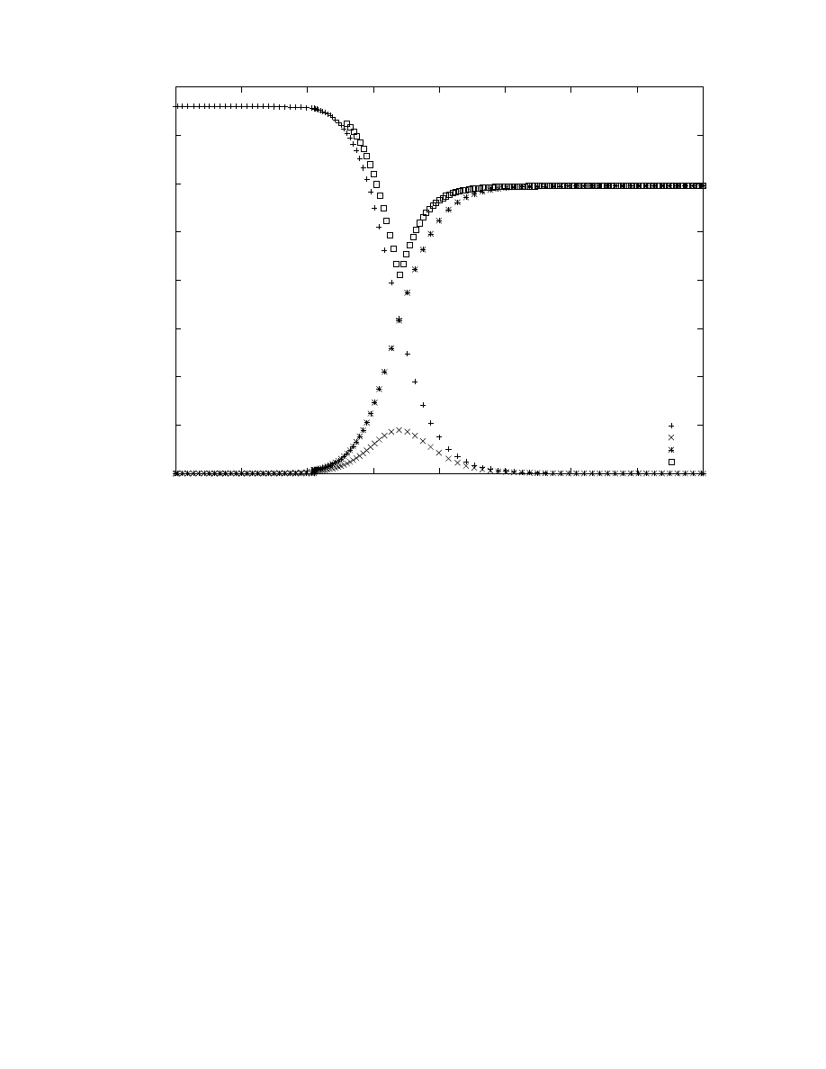
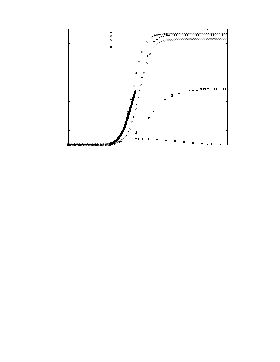
worm itself. Figure 3 plots the aggregate number of hosts
infected by time t, as a function of t, for the difference de-
fensive measures. We see that even though the simple patch
measure starts off with almost twice as many hosts as are
infected, the fact that that pool does not grow while the
infected set does means that the patching pool rescues rel-
atively few susceptible hosts. However, when the patching
pool can grow and when it starts with a pool size nearly
twice that of the infected set, we expect that approximately
2/3 of the hosts susceptible when the defenses start will be
saved from the worm (recall §4.1), and Figure 3 bears that
out. Of the hosts infected under the spreading patch de-
fense, about a third can be rescued when infection scanning
can be nullified, and roughly a third of the hosts infected
under a nullifying defense can be rescued when snipers are

used. There is almost a factor of 8 difference in the total
number of hosts infected by the worm between using no de-
fense at all, and using the most aggressive counter-worm
we’ve considered.

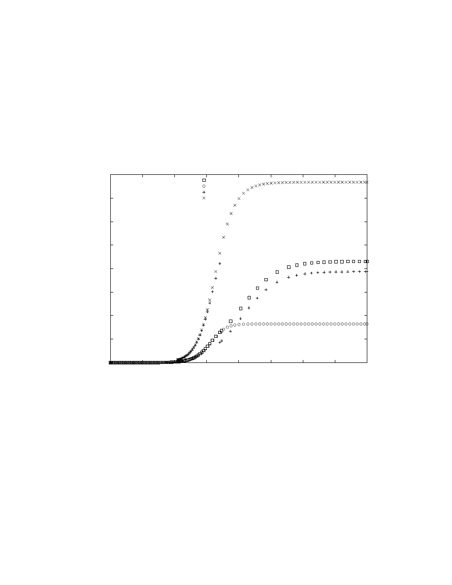
However, the total number of hosts infected is not the

only metric, and in some cases may not be the best met-
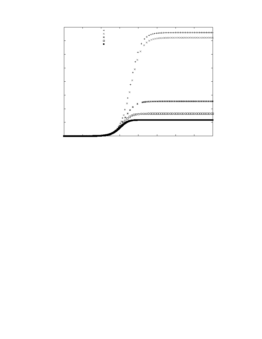
ric. In Figure 4 we plot the instantaneous total number of
hosts running either a worm, or a counter-worm; we assume
that the nullifying defense stops its counter scans nearly
optimally, and also show the effect of using that stopping
time for the sniper (which is optimally stopped earlier). The
spreading patch defense dominates the scan count, even the
empty defense—not only will every host eventually be run-
ning scans, there are an extra 3,800 hosts running counter
scans as well! The effect of stopping the counter-scans are
evident. Before the stopping time the nullifying defense’s
aggregate number of scanning hosts grows exponentially as
both the worm and counter-worm spread into susceptible
hosts. At the stopping time the number of scanning hosts
drops sharply, to reflect only the infected hosts. After the
stopping time this set is left unchecked by counter-scans, and
grows to reclaim all of the remaining susceptibles. From the
point of view of maximum number of hosts scanning, the op-
timal stopping time occurs when the peak of the scans just
at the stopping point is the same as the peak of the scans
after the stopping point. The sniper defense shows a similar
drop, but there are different post-stopping time dynamics—
because the pool of infected hosts is smaller than the pool

0

50000

100000

150000

200000

250000

300000

350000

400000

0

2

4

6

8

10

12

14

16

Infected Hosts

Hours

empty defense

simple patch

spreading patch

nullifying worm

sniper worm

Figure 3: Aggregate number of hosts ever infected

of counter-worm hosts, the infected pool will diminish with
time, because random scans from that pool are more likely to
encounter hosts with counter-worms than susceptible hosts.

A defense that seeks to miminize the peak number of hosts

scanning instantaneously (e.g., using a counter-scan stop-
ping time) may not minimize the number aggregate num-
ber of hosts that become infected (e.g., without a stopping
time), and vice-versa. We illustrate this point with Fig-
ure 5 where we plot the cumulative number of infected hosts,
and the instantaneous number of scanning hosts (includ-
ing counter-scans) under the nullifying defense, with and
without stopping.

The tradeoff between scanning inten-

sity and number of hosts ultimately infected is quite pro-
nounced. The non-stopping version continues scanning in
order to drive the infection count down. It is successful at
keeping the number of infected hosts down to about 1/4 of
the susceptible population, but at the cost of an extremely
high scanning intensity. The stopping version minimizes the
scanning intensity, but the price paid for that minimization
is a total infection count that is over twice as large as the
non-stopping version.

The ability to generate models of active defense behav-

ior is an invaluable way to understand what the costs and
benefits of active defenses are.

5.

CONCLUSIONS

This paper studies active defenses against Internet worms.

We use discrete and continuous mathematical models to
study a hierarchy of worm fighting capabilities. We are able
to prove a number of results about these models, including

• strong stochastic ordering of infection counts in a hi-

erarchy of five defense types;

• that a simple counter-worm defense has a stochasti-

cally larger aggregate scanning intensity than does the
unfettered worm;

• that by starting a defense with enough outside hosts

scanning to implant counter-worms, any desired frac-
tion of the remaining susceptible hosts can be pro-
tected from a worm;

• that by starting a nullifying defense with few enough

outside hosts, the peak scanning intensity is less than
the unfettered worm;

• even when peak scanning time is minimized under the

nullifying defense, it is still the case that the peak num-
ber of hosts scanning is at least 1/3 of the total number
of susceptibles;

In addition, we show by example how numerical solution

of the continous models quantifies the power of various ac-
tive defenses (in terms of hosts infected) and the cost (in
terms of scanning intensities). Ability to study worm be-
havior this way leads to better understanding of some of the
tradeoffs involved.

There is much work yet to be done. This paper does not

address the very significant problem of quickly and automat-
ically detecting when a worm attack has been launched—we
have looked only at the relative effectiveness of measures
put into place after the detection. Our experiments of effec-
tiveness of defense as a function of response time (Figure 1)
show that rapid detection is absolutely critical. The work

0

50000

100000

150000

200000

250000

300000

350000

400000

0

2

4

6

8

10

12

14

16

Infected Hosts

Hours

empty defense

simple patch

spreading patch

nullifying worm

sniper worm

Figure 4: Instantaneous number of hosts scanning, either worm or counter-worm

in this paper does not take network topology into considera-
tion. This latter issue must be address to adequately model
very fast worms, which experience has shown affect the net-
working infrastructure, and which one may expect are in
turn affected by the changes wrought on the infrastructure.

6.

REFERENCES

[1] Z. Chen, L. Gao, and K. Kwiat. Modeling the spread

of active worms. In INFOCOM 2003, 2003.

[2] Cisco. Dealing with mallocfail and high cpu utilization

resulting from the “code red” worm.
http://www.cisco.com/warp/public/-
63/ts codred worm.shtml, October
2001.

[3] D.J. Daley and J. Gani. Epidemic Modelling: An

Introduction. Cambridge University Press, Cambridge,
UK, 1999.

[4] P. Ferrie, F. Perriot, and P. Sz or. Worm wars. Virus

Bulletin

(www.virusbtn.com), Oct 2003.

http://www.peterszor.com/welchia.pdf

[Last

accessed Oct 01, 2003.

[5] M. Liljenstam, D. Nicol, V. Berk, and B. Gray.

Simulating realistic network worm traffic for worm
warning system design and testing. In in Proc. of the
First ACM Workshop on Rapid Malcode (WORM’03),
Oct 2003.

[6] D. Moore, C. Shannon, and K. Claffy. Code-red: a

case study on the spread and victims of an internet
worm. In in Proc. of the Internet Measurement
Workshop (IMW), Marseille, France, Nov 2002. ACM
Press.

[7] D. Moore, C. Shannon, G. Voelker, and S. Savage.

Internet quarantine: Requirements for containing
self-propagating code. In Proceedings of the 22nd
Annual Joint Conference of the IEEE Computer and
Communications Societies (INFOCOM 2003), April
2003.

[8] H.S. Ross. Stochastic Processes. Wiley, New York,

1983.

[9] S. Staniford. Code Red Analysis Pages: July

infestation analysis.
http://www.silicondefense.com/cr/july.html, 2001.

[10] S. Staniford, V. Paxson, and N. Weaver. How to Own

the Internet in Your Spare Time. In in Proc. of the
USENIX Security Symposium, 2002.
http://www.icir.org/vern/papers/cdc-usenix-
sec02/index.html.

[11] C. Zou, L. Gao, W. Gong, and D. Towsley. Code red

worm propagation modeling and analysis. In 9th ACM
Conference on Computer and Communication Security
(CCS), Washington DC, Nov 2002.

[12] C. Zou, L. Gao, W. Gong, and D. Towsley. Monitoring

and early warning for internet worms. In Proceedings
of 10th ACM Conference on Computer and
Communication Security (CCS’03), 2003.

[13] C. Zou, W. Gong, and D. Towsley. Worm propagation

modeling and analysis. In Proceedings of the First
ACM Workshop on Rapid Malcode (WORM), 2003.

0

50000

100000

150000

200000

250000

300000

350000

400000

0

2

4

6

8

10

12

14

16

Infected Hosts

Hours

infected, stopping

infected, non-stopping

scanning, stopping

scanning, non-stopping

Figure 5: Total number of hosts infected, and instantaneous number of hosts scanning, as a function of time,
for the nullifying defense, with and without stopping counter scans.