690-264A

SCHAFFNER

CISPR 17 Measurements

50

Ω / 50Ω versus 0.1Ω / 100Ω

The truth

or

Everything you wanted to know

about attenuation curves validity

but were afraid to ask

A practical study using the

FN 9675-3-06 power line filter

SCHAFFNER

CISPR 17 Measurements

Schaffner EMV AG CH-4542 Luterbach/Switzerland

SCHAFFNER

2

1

Introduction

The use of power line filter insertion loss/attenuation curve data (as published by filter
manufacturers) has been a frustrating experience to less experienced EMC engineers
for a very long time.

Engineers with extensive experience in EMC consider these curves, generally prepared
from data taken in a 50

Ω

test setup, to be of extremely limited value. In spite of this,

filter manufacturers continue to publish 50

Ω

data, since popular 50

Ω

equipment,

connectors and test cables make these the most easily taken measurements.

Attenuation curves using 50

Ω

impedance are severely criticized in many books and

technical papers as well as in insertion loss measurement standards such as Mil Std
220A and CISPR 17.

CISPR 17 gives several alternatives to 50

Ω

insertion loss measurment curves. These

alternatives are aimed at showing the filter effectiveness in real situations rather than
in an artificial situation.

The cause of the problem is that in real life situations, a power line filter is not
terminated with 50

Ω

impedances. In fact, the filter termination is usually an unknown

value that often changes with frequency. Since the filter performance is largely
dependent upon termination impedance, the curves given in 50

Ω

can never represent

the real live situation.

2

Alternatives to 50

Ω measurement

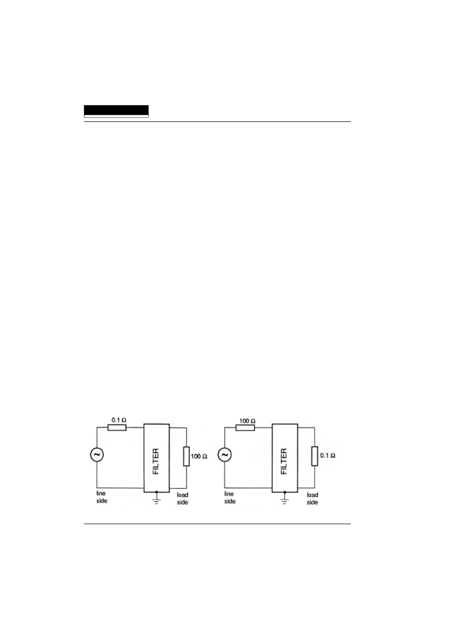
One of the alternatives given in CISPR 17 is the so called "Approximate Worst Case
Method".

In this test method the filter insertion loss is measured with 0.1

Ω

and 100

Ω

terminations

on the line and load side, respectively. The measurements are then repeated with the
terminating impedances reversed.

Fig. 1 "Approximate Worst Case" test diagram

SCHAFFNER

3

Although this test method is not the same as measuring a filter in a real equipment
installation, the normalized results can be used with relative accuracy to predict the
performance of the filter in a real situation. Another advantage is that it is a well defined
standard measuring method from CISPR. This test yields accurate and repeatable
results.

The power line filter industry must publish data on its products using recognised,
standardized and accepted test methods. If, as generally accepted, the 50

Ω

method

cannot be used to predict the performance of a filter in real equipment, the CISPR 17
"Approximate Worst Case" method is the only such standardized test to meet this
requirement.

3

How to use 0.1

Ω / 100Ω data

SCHAFFNER has conducted tests on many different interference sources in real
equipment with and without a filter. A statistical analysis of the results of noise
measurements with and without the filter gives the "Effective Attenuation" of that filter.
Unfortunately, a filter customer is rarely able to make such complex measurements and
must normally rely on predictions from published data.

When this "Effective Attenuation" data is compared to attenuation curves taken using
the 50

Ω

/50

Ω

and the 0.1

Ω

/100

Ω

methods, the latter is clearly seen to more nearly

portray the real performance of the filter.

The 50

Ω

/50

Ω

attenuation curve will consistently show higher levels of performance

than actually achieved, sometimes by significant amounts. The 0.1

Ω

/100

Ω

attenuation

is normally slightly less than the real "Effective Attenuation", although often by only
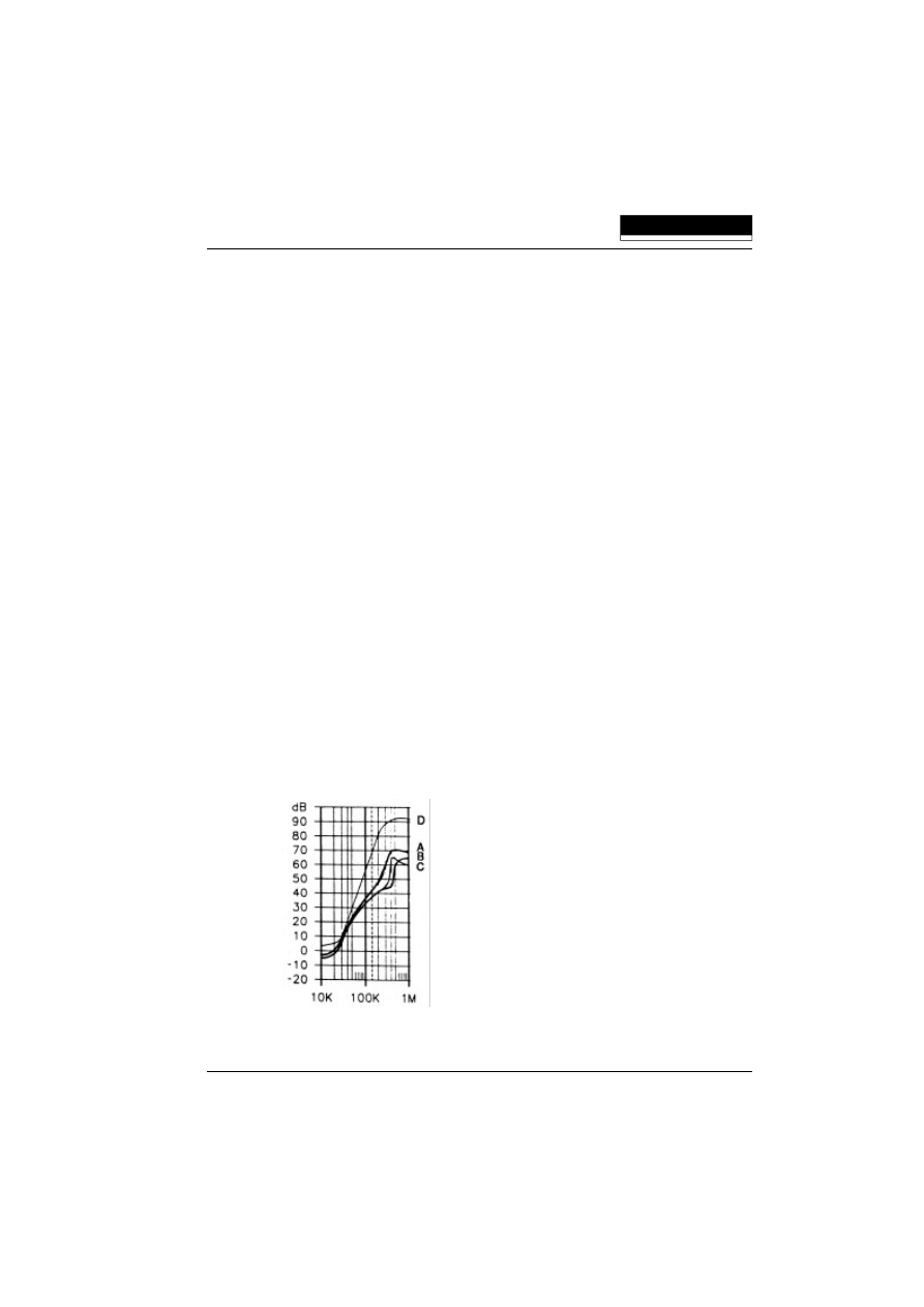
a few dB. Fig. 2 below shows the results for a SCHAFFNER FN 9675-3 line filter.

Curve A
Effective system attenuation

Curve B
0.1

Ω

/100

Ω

attenuation measurement

Curve C
100

Ω

/0.1

Ω

attenuation measurement

Curve D
50

Ω

/50

Ω

attenuation measurement

Fig. 2 FN 9675-3 differential mode data

SCHAFFNER

4

In Fig. 2 the data cover the lower frequency range up to 1MHz. The data presented for
the 50

Ω

/50

Ω

and 0.1

Ω

/100

Ω

methods are those measured in the differential or

"symmetrical" mode. In this frequency range the "Effective Attenuation" as measured
corresponds closely to the symmetrical attenuation curve.

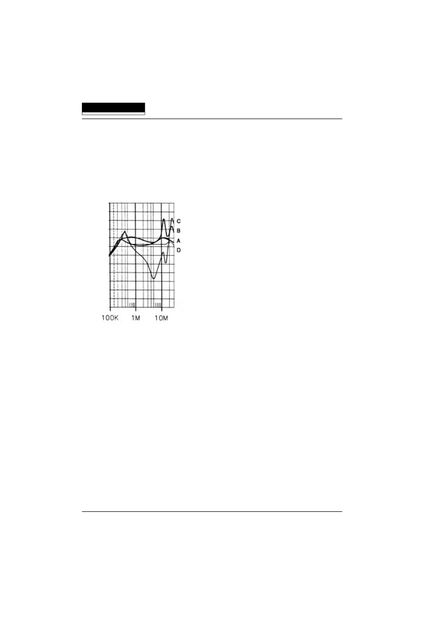
Above 1MHz, the common mode or "asymmetrical" mode attenuation is found to be
more important. In some cases common mode attenuation data is also useful at lower
frequencies.

Curve A
Effective system attenuation

Curve B
0.1

Ω

/100

Ω

attenuation measurement

Curve C
100

Ω

/0.1

Ω

attenuation measurement

Curve D
50

Ω

/50

Ω

attenuation measurement

Fig. 3 FN 9675-3 common mode data

Fig. 3 shows that in this higher frequency range the "Effective Attenuation" corresponds
closely to the common mode or "asymmetrical" curve. Of course, in an actual analysis
of a real customer's product, if it is possible to determine if the system under test has
a low or a high input impedance, a choice can be made between the 0.1

Ω

/100

Ω

curve

and the 100

Ω

/0.1

Ω

curve for even better correllation.

Obviously, at frequencies above a few MHz, normal EMC practices are required to
insure optimum filter performance. This includes a reduction of all coupling paths
across the filter. The proper application of bonding, grounding, cable routing and filter
positioning techniques will optimize filter performance.

Fig. 2 shows the differential mode with a negative insertion loss, that is an insertion
gain! This happens relatively often in practice. It would be unwise to try to use such
a filter in an equipment with a discrete interference frequency falling within this region,
but only 0.1

Ω

/100

Ω

attenuation data will help a designer spot this problem beforehand.

In the common mode data of Fig. 3 the 0.1

Ω

/100

Ω

curve is very different from the 100

Ω

/

0.1

Ω

curve. This kind of difference can also exist in the differential mode, depending

on the actual configuration of the filter.

SCHAFFNER

5

The common mode curve C shows a dip in the insertion loss at 6MHz. A similar
resonance was seen during testing in our lab when a filter was mounted in the
equipment "the wrong way", with the Y caps on the line side. This may explain why Y
caps are usually placed on the load side of a filter. But the 0.1

Ω

/100

Ω

curves allow you

to see that a potential problem exists that you would not have seen with 50

Ω

data.

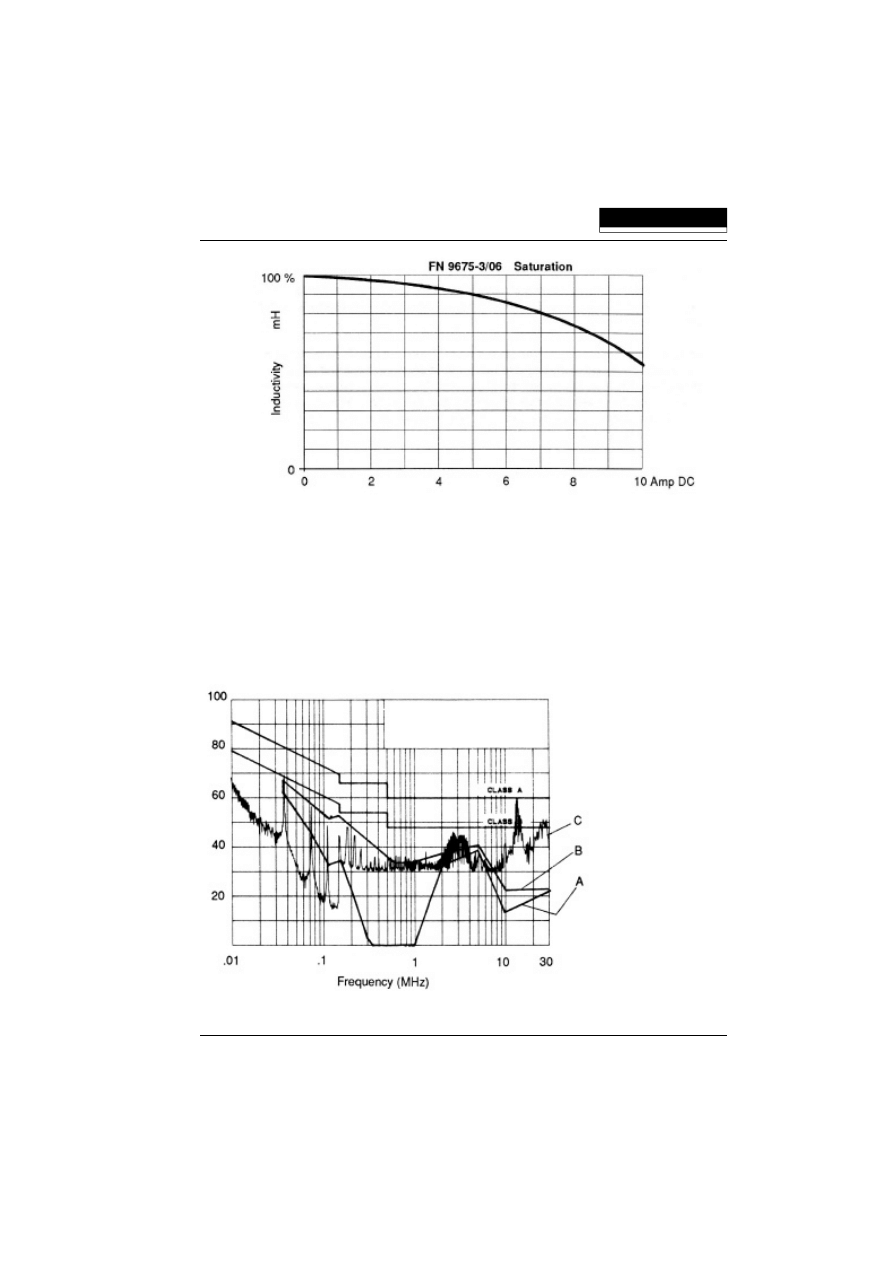
4

Saturation current

The 0.1

Ω

/100

Ω

curves shown above are taken without load. The change in inductance

with load current is shown separately. This is another simple and repeatable test.

We recommend that the line current wave shape of the equipment under test be
measured using an oscilloscope and current probe before the filter is installed. The
most important measurement is that of the peak current the filter must sustain.

Relating this peak current to the saturation curve of the filter will show what percentage
of the inductance remains at that current. If there is little change in the inductance at
that peak current, you can use the 0.1

Ω

/100

Ω

curves as they are.

If the inductance falls by up to 50%, then you need to allow for a variation of up to 6dB
in the attenuation given in the 0.1

Ω

/100

Ω

curves. We recommend that you consider

another filter if the inductance falls by more than 50%.

Fig. 4 Saturation curve

Filters from SCHAFFNER are designed for stable inductance over the normal ranges
of peak to RMS current ratios found in today's capacitor input power supply circuits.

SCHAFFNER

6

5

An example

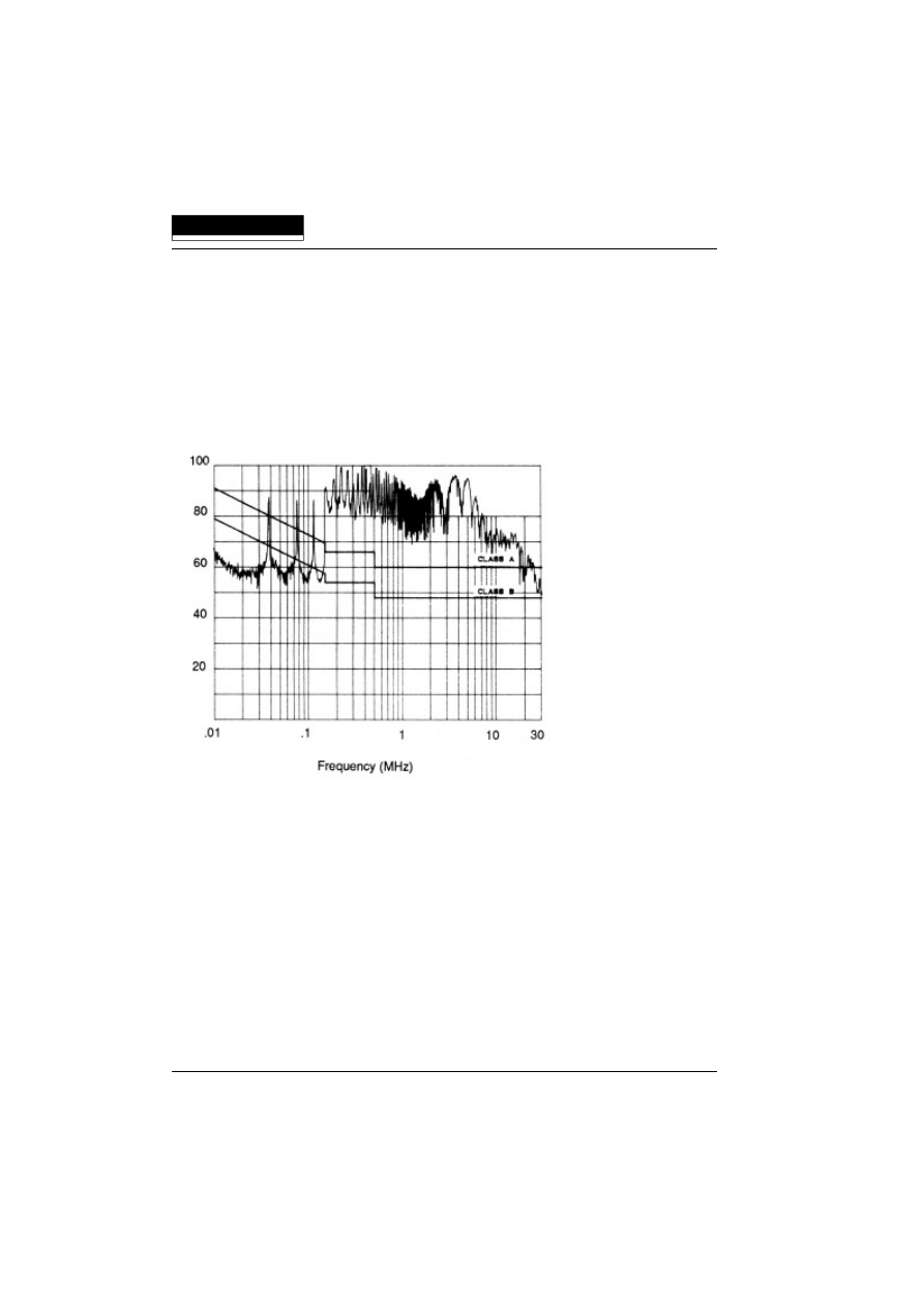
Fig. 5 shows an EMI test curve of the noise output of a typical switched-mode power
supply (SMPS). The noise limits of the VDE specification are also shown.

Using an oscilloscope, the line current was measured to have a peak value of 3.5A,
which compares to the 1.1A measured with an RMS-reading meter. This peak to RMS
ratio (or "Crest Factor") of 3.2:1 is typical for a SMPS, and much higher than the 1.4:1
ratio obtained on a resistive load. Inrush current (on startup) was greater than 15A.

Fig. 5 Noise output of a typical SMPS

In this example we would like to use the FN 9675-3-06, a high performace filter rated
for a maximum RMS line current of 0.3A. The saturation curves for this filter is shown
in Fig. 6. At the peak current of 3.5A there is still more than 95% of the inductance
present. The 0.1

Ω

/100

Ω

curve for this filter is shown in Fig. 2 and Fig. 3.

SCHAFFNER

7

Fig. 6 Saturation curve for a FN 9675-3-06

Using the symmetrical attenuation (differential mode) data for less than 1MHz and the
asymmetrical attenuation (common mode) data for above 1MHz, a prediction of the
noise output of the equipment with the filter can be made.

The result is shown in Fig. 7, together with an actual noise test taken with the filter in
the equipment. In the region below 10MHz the prediction corresponds almost exactly
to the actual results.

Fig. 7 Noise level prediction vs. results

Curve

A

Noise level prediction with 50

Ω

curves

Curve

B

Noise level prediction with 0.1

Ω

/100

Ω

curves

Curve

C

Real system noise level after filtering

SCHAFFNER

8

In general, the actual system noise after filtering is usually found to be below the system
noise level prediction using the 0.1

Ω

/100

Ω

method. At frequencies above 10MHz,

coupling effects can bypass the filter and give an unrealistic shape to the attenuation
curves.

Also shown is a system prediction based on 50

Ω

test curves. At low frequencies, which

is a very critical region in this application, these show a deviation of up to 20dB from
the actual results. Had we based the filter selection on 50

Ω

curves, a smaller, cheaper

and ineffective filter would have appeared sufficient. This would have lead to time
wasted on the unnecessary evaluation of the "wrong" filter, or to a system design that
failed qualification testing.

Corporate Headquarters

Schaffner EMV AG
Nordstrasse 11
CH-4542 Luterbach/Switzerland
Phone [phone]
Fax

[phone]

Subsidiary companies

China

Finland

Schaffner Beijing Liaison Office

Schaffner Electro Ferrum Oy

Phone [phone]

Phone [phone]

Fax

[phone]

Fax

[phone]

France

Germany

Schaffner EMC S.A.S.

Schaffner EMV GmbH

Phone [phone]

Phone [phone]

Fax

[phone]

Fax

[phone]

Italy

Japan

Schaffner EMC S.r.l.

Schaffner EMC K.K.

Phone [phone]

Phone [phone]

Fax

[phone]

Fax

[phone]

Singapore

Sweden

Schaffner EMC Pte. Ltd.

Schaffner EMC AB

Phone [phone]

Phone [phone]

Fax

[phone]

Fax

[phone]

Switzerland

United Kingdom

Schaffner EMV AG

Schaffner EMC Ltd.

Phone [phone]

Phone [phone]

Fax

[phone]

Fax

[phone]

USA
Schaffner EMC Inc.
Phone [phone]
Fax

[phone]

Albrecht/March 1996

SCHAFFNER