EURACHEM CITAC Wyrażanie niepewności pomiaru analitycznego, wyd 2, 2000

EURACHEM / CITAC Guide CG 4

Quantifying Uncertainty in

Analytical Measurement

Second Edition

QUAM:2000.1

EURACHEM/CITAC Guide*

Quantifying Uncertainty in
Analytical Measurement

Second Edition

Editors

S L R Ellison (LGC, UK)
M Rosslein (EMPA, Switzerland)
A Williams (UK)

Composition of the Working Group

EURACHEM members

A Williams Chairman

S EllisonSecretary

LGC, Teddington, UK

M Berglund

Institute for Reference Materials and
Measurements, Belgium

W Haesselbarth

Bundesanstalt fur Materialforschung und
Prufung, Germany

K Hedegaard

EUROM II

R Kaarls

Netherlands Measurement Institute, The
Netherlands

M Månsson

SP Swedish National Testing and Research
Institute, Sweden

M Rösslein

EMPA St. Gallen, Switzerland

R Stephany

National Institute of Public Health and the
Environment, The Netherlands

A van der Veen

Netherlands Measurement Institute, The
Netherlands

W Wegscheider

University of Mining and Metallurgy, Leoben,
Austria

H van de Wiel

National Institute of Public Health and the
Environment, The Netherlands

R Wood

Food Standards Agency, UK

CITAC Members

Pan Xiu Rong

Director, NRCCRM,. China

M Salit

National Institute of Science and Technology
USA

A Squirrell

NATA, Australia

K Yasuda

Hitachi Ltd, Japan

AOAC Representatives

R Johnson

Agricultural Analytical Services, Texas State
Chemist, USA

Jung-Keun Lee

U.S. F.D.A. Washington

D Mowrey

Eli Lilly & Co., Greenfield, USA

IAEA Representatives

P De Regge

IAEA Vienna

A Fajgelj

IAEA Vienna

EA Representative

D Galsworthy,

UKAS, UK

Acknowledgements

This document has been produced primarily by a joint
EURACHEM/CITAC Working Group with the
composition shown (right). The editors are grateful to
all these individuals and organisations and to others
who have contributed comments, advice and
assistance.

Production of this Guide was in part supported under
contract with the UK Department of Trade and
Industry as part of the National Measurement System
Valid Analytical Measurement (VAM) Programme.

*CITAC Reference
This Guide constitutes CITAC Guide number 4

Quantifying Uncertainty in Analytical Measurement

English edition

Second edition 2000

ISBN 0 948926 15 5

 2000

Quantifying Uncertainty

Contents

QUAM:2000.1

Page i

CONTENTS

FOREWORD TO THE SECOND EDITION

1. SCOPE AND FIELD OF APPLICATION

2. UNCERTAINTY

2.1. D

EFINITION OF UNCERTAINTY

2.2. U

NCERTAINTY SOURCES

2.3. U

NCERTAINTY COMPONENTS

2.4. E

RROR AND UNCERTAINTY

3. ANALYTICAL MEASUREMENT AND UNCERTAINTY

3.1. M

ETHOD VALIDATION

3.2. C

ONDUCT OF EXPERIMENTAL STUDIES OF METHOD PERFORMANCE

3.3. T

RACEABILITY

4. THE PROCESS OF MEASUREMENT UNCERTAINTY ESTIMATION

5. STEP 1. SPECIFICATION OF THE MEASURAND

6. STEP 2. IDENTIFYING UNCERTAINTY SOURCES

7. STEP 3. QUANTIFYING UNCERTAINTY

7.1. I

NTRODUCTION

7.2. U

NCERTAINTY EVALUATION PROCEDURE

7.3. R

ELEVANCE OF PRIOR STUDIES

7.4. E

VALUATING UNCERTAINTY BY QUANTIFICATION OF INDIVIDUAL COMPONENTS

7.5. C

LOSELY MATCHED CERTIFIED REFERENCE MATERIALS

7.6. U

SING PRIOR COLLABORATIVE METHOD DEVELOPMENT AND VALIDATION STUDY DATA

7.7. U

SING IN

HOUSE DEVELOPMENT AND VALIDATION STUDIES

7.8. E

VALUATION OF UNCERTAINTY FOR EMPIRICAL METHODS

7.9. E

VALUATION OF UNCERTAINTY FOR AD

HOC METHODS

7.10. Q

UANTIFICATION OF INDIVIDUAL COMPONENTS

7.11. E

XPERIMENTAL ESTIMATION OF INDIVIDUAL UNCERTAINTY CONTRIBUTIONS

7.12. E

STIMATION BASED ON OTHER RESULTS OR DATA

7.13. M

ODELLING FROM THEORETICAL PRINCIPLES

7.14. E

STIMATION BASED ON JUDGEMENT

7.15. S

IGNIFICANCE OF BIAS

8. STEP 4. CALCULATING THE COMBINED UNCERTAINTY

8.1. S

TANDARD UNCERTAINTIES

8.2. C

OMBINED STANDARD UNCERTAINTY

8.3. E

XPANDED UNCERTAINTY

Quantifying Uncertainty

Contents

QUAM:2000.1

Page ii

9. REPORTING UNCERTAINTY

9.1. G

ENERAL

9.2. I

NFORMATION REQUIRED

9.3. R

EPORTING STANDARD UNCERTAINTY

9.4. R

EPORTING EXPANDED UNCERTAINTY

9.5. N

UMERICAL EXPRESSION OF RESULTS

9.6. C

OMPLIANCE AGAINST LIMITS

APPENDIX A. EXAMPLES

NTRODUCTION

XAMPLE

A1: P

REPARATION OF A

ALIBRATION

TANDARD

XAMPLE

A2: S

TANDARDISING A

ODIUM

YDROXIDE

OLUTION

XAMPLE

A3: A

CID

ASE

ITRATION

XAMPLE

A4: U

NCERTAINTY

STIMATION FROM

-H

OUSE

ALIDATION

TUDIES

ETERMINATION OF

RGANOPHOSPHORUS

ESTICIDES IN

READ

XAMPLE

A5: D

ETERMINATION OF

ADMIUM

ELEASE FROM

ERAMIC

ARE BY

TOMIC

BSORPTION

PECTROMETRY

XAMPLE

A6: T

ETERMINATION OF

RUDE

IBRE IN

NIMAL

EEDING

TUFFS

XAMPLE

A7: D

ETERMINATION OF THE

MOUNT OF

EAD IN

ATER

SING

OUBLE

SOTOPE

ILUTION AND

NDUCTIVELY

OUPLED

LASMA

ASS

PECTROMETRY

APPENDIX B. DEFINITIONS

APPENDIX C. UNCERTAINTIES IN ANALYTICAL PROCESSES

APPENDIX D. ANALYSING UNCERTAINTY SOURCES

100

D.1

NTRODUCTION

100

D.2

RINCIPLES OF APPROACH

100

D.3

AUSE AND EFFECT ANALYSIS

100

D.4

XAMPLE

101

APPENDIX E. USEFUL STATISTICAL PROCEDURES

102

E.1

ISTRIBUTION FUNCTIONS

102

E.2

PREADSHEET METHOD FOR UNCERTAINTY CALCULATION

104

E.3

NCERTAINTIES FROM LINEAR LEAST SQUARES CALIBRATION

106

E.4: D

OCUMENTING UNCERTAINTY DEPENDENT ON ANALYTE LEVEL

108

APPENDIX F. MEASUREMENT UNCERTAINTY AT THE LIMIT OF DETECTION/
LIMIT OF DETERMINATION

112

F1.

NTRODUCTION

112

F2.

BSERVATIONS AND ESTIMATES

112

F3.

NTERPRETED RESULTS AND COMPLIANCE STATEMENTS

113

APPENDIX G. COMMON SOURCES AND VALUES OF UNCERTAINTY

114

APPENDIX H. BIBLIOGRAPHY

120

Quantifying Uncertainty

QUAM:2000.1

Page 1

Foreword to the Second Edition

Many important decisions are based on the results of chemical quantitative analysis; the results are used, for
example, to estimate yields, to check materials against specifications or statutory limits, or to estimate
monetary value. Whenever decisions are based on analytical results, it is important to have some indication
of the quality of the results, that is, the extent to which they can be relied on for the purpose in hand. Users
of the results of chemical analysis, particularly in those areas concerned with international trade, are coming
under increasing pressure to eliminate the replication of effort frequently expended in obtaining them.
Confidence in data obtained outside the user’s own organisation is a prerequisite to meeting this objective.
In some sectors of analytical chemistry it is now a formal (frequently legislative) requirement for
laboratories to introduce quality assurance measures to ensure that they are capable of and are providing
data of the required quality. Such measures include: the use of validated methods of analysis; the use of
defined internal quality control procedures; participation in proficiency testing schemes; accreditation based
on ISO 17025 [H.1], and establishing traceability of the results of the measurements

In analytical chemistry, there has been great emphasis on the precision of results obtained using a specified
method, rather than on their traceability to a defined standard or SI unit. This has led the use of “official
methods” to fulfil legislative and trading requirements. However as there is now a formal requirement to
establish the confidence of results it is essential that a measurement result is traceable to a defined reference
such as a SI unit, reference material or, where applicable, a defined or empirical (sec. 5.2.) method. Internal
quality control procedures, proficiency testing and accreditation can be an aid in establishing evidence of
traceability to a given standard.

As a consequence of these requirements, chemists are, for their part, coming under increasing pressure to
demonstrate the quality of their results, and in particular to demonstrate their fitness for purpose by giving a
measure of the confidence that can be placed on the result. This is expected to include the degree to which a
result would be expected to agree with other results, normally irrespective of the analytical methods used.
One useful measure of this is measurement uncertainty.

Although the concept of measurement uncertainty has been recognised by chemists for many years, it was
the publication in 1993 of the “Guide to the Expression of Uncertainty in Measurement” [H.2] by ISO in
collaboration with BIPM, IEC, IFCC, IUPAC, IUPAP and OIML, which formally established general rules
for evaluating and expressing uncertainty in measurement across a broad spectrum of measurements. This
EURACHEM document shows how the concepts in the ISO Guide may be applied in chemical
measurement. It first introduces the concept of uncertainty and the distinction between uncertainty and
error. This is followed by a description of the steps involved in the evaluation of uncertainty with the
processes illustrated by worked examples in Appendix A.

The evaluation of uncertainty requires the analyst to look closely at all the possible sources of uncertainty.
However, although a detailed study of this kind may require a considerable effort, it is essential that the
effort expended should not be disproportionate. In practice a preliminary study will quickly identify the
most significant sources of uncertainty and, as the examples show, the value obtained for the combined
uncertainty is almost entirely controlled by the major contributions. A good estimate of uncertainty can be
made by concentrating effort on the largest contributions. Further, once evaluated for a given method
applied in a particular laboratory (i.e. a particular measurement procedure), the uncertainty estimate
obtained may be reliably applied to subsequent results obtained by the method in the same laboratory,
provided that this is justified by the relevant quality control data. No further effort should be necessary
unless the procedure itself or the equipment used is changed, in which case the uncertainty estimate would
be reviewed as part of the normal re-validation.

The first edition of the EURACHEM Guide for “Quantifying Uncertainty in Analytical Measurement” [H.3]
was published in 1995 based on the ISO Guide.

Quantifying Uncertainty

Foreword to the Second Edition

QUAM:2000.1

Page 2

This second edition of the EURACHEM Guide has been prepared in the light of practical experience of
uncertainty estimation in chemistry laboratories and the even greater awareness of the need to introduce
formal quality assurance procedures by laboratories. The second edition stresses that the procedures
introduced by a laboratory to estimate its measurement uncertainty should be integrated with existing
quality assurance measures, since these measures frequently provide much of the information required to
evaluate the measurement uncertainty. The guide therefore provides explicitly for the use of validation and
related data in the construction of uncertainty estimates in full compliance with formal ISO Guide
principles. The approach is also consistent with the requirements of ISO 17025:1999 [H.1]

OTE

Worked examples are given in Appendix A. A numbered list of definitions is given at Appendix B. The
convention is adopted of printing defined terms in bold face upon their first occurrence in the text, with a
reference to Appendix B enclosed in square brackets. The definitions are, in the main, taken from the
International vocabulary of basic and general standard terms in Metrology (VIM) [H.4], the Guide [H.2] and
ISO 3534 (Statistics - Vocabulary and symbols) [H.5]. Appendix C shows, in general terms, the overall
structure of a chemical analysis leading to a measurement result. Appendix D describes a general procedure
which can be used to identify uncertainty components and plan further experiments as required; Appendix E
describes some statistical operations used in uncertainty estimation in analytical chemistry. Appendix F
discusses measurement uncertainty near detection limits. Appendix G lists many common uncertainty sources
and methods of estimating the value of the uncertainties. A bibliography is provided at Appendix H.

Quantifying Uncertainty

Scope and Field of Application

QUAM:2000.1

Page 3

1. Scope and Field of Application

1.1.

This Guide gives detailed guidance for the evaluation and expression of uncertainty in quantitative

chemical analysis, based on the approach taken in the ISO “Guide to the Expression of Uncertainty in
Measurement” [H.2]. It is applicable at all levels of accuracy and in all fields - from routine analysis to
basic research and to empirical and rational methods (see section 5.3.). Some common areas in which
chemical measurements are needed, and in which the principles of this Guide may be applied, are:

•

Quality control and quality assurance in manufacturing industries.

•

Testing for regulatory compliance.

•

Testing utilising an agreed method.

•

Calibration of standards and equipment.

•

Measurements associated with the development and certification of reference materials.

•

Research and development.

1.2.

Note that additional guidance will be required in some cases. In particular, reference material value

assignment using consensus methods (including multiple measurement methods) is not covered, and the use
of uncertainty estimates in compliance statements and the expression and use of uncertainty at low levels
may require additional guidance. Uncertainties associated with sampling operations are not explicitly
treated.

1.3.

Since formal quality assurance measures have been introduced by laboratories in a number of sectors

this second EURACHEM Guide is now able to illustrate how data from the following procedures may be
used for the estimation of measurement uncertainty:

•

Evaluation of the effect of the identified sources of uncertainty on the analytical result for a single

method implemented as a defined measurement procedure [B.8] in a single laboratory .

•

Results from defined internal quality control procedures in a single laboratory.

•

Results from collaborative trials used to validate methods of analysis in a number of competent

laboratories.

•

Results from proficiency test schemes used to assess the analytical competency of laboratories.

1.4. It is assumed throughout this Guide that, whether carrying out measurements or assessing the
performance of the measurement procedure, effective quality assurance and control measures are in place to
ensure that the measurement process is stable and in control. Such measures normally include, for example,
appropriately qualified staff, proper maintenance and calibration of equipment and reagents, use of
appropriate reference standards, documented measurement procedures and use of appropriate check
standards and control charts. Reference [H.6] provides further information on analytical QA procedures.

OTE

: This paragraph implies that all analytical methods are assumed in this guide to be implemented via fully

documented procedures. Any general reference to analytical methods accordingly implies the presence of such
a procedure. Strictly, measurement uncertainty can only be applied to the results of such a procedure and not to
a more general method of measurement [B.9].

Quantifying Uncertainty

Uncertainty

QUAM:2000.1

Page 4

2. Uncertainty

2.1. Definition of uncertainty

2.1.1. The definition of the term uncertainty (of
measurement) used in this protocol and taken
from the current version adopted for the
International Vocabulary of Basic and General
Terms in Metrology [H.4] is:

“A parameter associated with the result of a
measurement, that characterises the dispersion of
the values that could reasonably be attributed to
the measurand”

Note

The parameter may be, for example, a
standard deviation [B.23] (or a given
multiple of it), or the width of a confidence
interval.

OTE

2 Uncertainty of measurement comprises, in

general, many components. Some of these
components may be evaluated from the
statistical distribution of the results of series
of measurements and can be characterised by
standard deviations. The other components,
which also can be characterised by standard
deviations, are evaluated from assumed
probability distributions based on experience
or other information. The ISO Guide refers to
these different cases as Type A and Type B
estimations respectively.

2.1.2. In many cases in chemical analysis, the
measurand [B.6] will be the concentration

of an

analyte. However chemical analysis is used to
measure other quantities, e.g. colour, pH, etc.,
and therefore the general term "measurand" will
be used.

2.1.3. The definition of uncertainty given above
focuses on the range of values that the analyst
believes could reasonably be attributed to the
measurand.

2.1.4. In general use, the word uncertainty relates
to the general concept of doubt. In this guide, the

In this guide, the unqualified term “concentration”

applies to any of the particular quantities mass
concentration,

amount concentration, number

concentration or volume concentration unless units
are quoted (e.g. a concentration quoted in mg l

-1

evidently a mass concentration). Note also that many
other quantities used to express composition, such as
mass fraction, substance content and mole fraction,
can be directly related to concentration.

word uncertainty, without adjectives, refers either
to a parameter associated with the definition
above, or to the limited knowledge about a
particular value. Uncertainty of measurement
does not imply doubt about the validity of a
measurement; on the contrary, knowledge of the
uncertainty implies increased confidence in the
validity of a measurement result.

2.2. Uncertainty sources

2.2.1. In practice the uncertainty on the result
may arise from many possible sources, including
examples such as incomplete definition,
sampling, matrix effects and interferences,
environmental conditions, uncertainties of masses
and volumetric equipment, reference values,
approximations and assumptions incorporated in
the measurement method and procedure, and
random variation (a fuller description of
uncertainty sources is given in section 6.7.)

2.3. Uncertainty components

2.3.1. In estimating the overall uncertainty, it may
be necessary to take each source of uncertainty
and treat it separately to obtain the contribution
from that source. Each of the separate
contributions to uncertainty is referred to as an
uncertainty component. When expressed as a
standard deviation, an uncertainty component is
known as a standard uncertainty [B.13]. If
there is correlation between any components then
this has to be taken into account by determining
the covariance. However, it is often possible to
evaluate the combined effect of several
components. This may reduce the overall effort
involved and, where components whose
contribution is evaluated together are correlated,
there may be no additional need to take account
of the correlation.

2.3.2. For a measurement result y, the total
uncertainty, termed combined standard
uncertainty [B.14] and denoted by u

(y), is an

estimated standard deviation equal to the positive
square root of the total variance obtained by
combining all the uncertainty components,
however evaluated, using the law of propagation
of uncertainty (see section 8.).

Quantifying Uncertainty

Uncertainty

QUAM:2000.1

Page 5

2.3.3. For most purposes in analytical chemistry,
an expanded uncertainty [B.15] U, should be
used. The expanded uncertainty provides an
interval within which the value of the measurand
is believed to lie with a higher level of
confidence. U is obtained by multiplying u

(y),

the combined standard uncertainty, by a coverage
factor [B.16] k. The choice of the factor k is
based on the level of confidence desired. For an
approximate level of confidence of 95

, k is 2.

OTE

The coverage factor k should always be stated
so that the combined standard uncertainty of
the measured quantity can be recovered for
use in calculating the combined standard
uncertainty of other measurement results that
may depend on that quantity.

2.4. Error and uncertainty

2.4.1. It is important to distinguish between error
and uncertainty. Error [B.19] is defined as the
difference between an individual result and the
true value [B.3] of the measurand. As such,
error is a single value. In principle, the value of a
known error can be applied as a correction to the
result.

OTE

Error is an idealised concept and errors cannot
be known exactly.

2.4.2. Uncertainty, on the other hand, takes the
form of a range, and, if estimated for an analytical
procedure and defined sample type, may apply to
all determinations so described. In general, the
value of the uncertainty cannot be used to correct
a measurement result.

2.4.3. To illustrate further the difference, the
result of an analysis after correction may by
chance be very close to the value of the
measurand, and hence have a negligible error.
However, the uncertainty may still be very large,
simply because the analyst is very unsure of how
close that result is to the value.

2.4.4. The uncertainty of the result of a
measurement should never be interpreted as
representing the error itself, nor the error
remaining after correction.

2.4.5. An error is regarded as having two
components, namely, a random component and a
systematic component.

2.4.6. Random error [B.20] typically arises from
unpredictable variations of influence quantities.
These random effects give rise to variations in
repeated observations of the measurand. The

random error of an analytical result cannot be
compensated for, but it can usually be reduced by
increasing the number of observations.

OTE

1 The experimental standard deviation of the

arithmetic mean [B.22] or average of a series
of observations is not the random error of the
mean, although it is so referred to in some
publications on uncertainty. It is instead a
measure of the uncertainty of the mean due to
some random effects. The exact value of the
random error in the mean arising from these
effects cannot be known.

2.4.7. Systematic error [B.21] is defined as a
component of error which, in the course of a
number of analyses of the same measurand,
remains constant or varies in a predictable way.
It is independent of the number of measurements
made and cannot therefore be reduced by
increasing the number of analyses under constant
measurement conditions.

2.4.8. Constant systematic errors, such as failing
to make an allowance for a reagent blank in an
assay, or inaccuracies in a multi-point instrument
calibration, are constant for a given level of the
measurement value but may vary with the level of
the measurement value.

2.4.9. Effects which change systematically in
magnitude during a series of analyses, caused, for
example by inadequate control of experimental
conditions, give rise to systematic errors that are
not constant.

EXAMPLES:

1. A gradual increase in the temperature of a set
of samples during a chemical analysis can lead
to progressive changes in the result.

2. Sensors and probes that exhibit ageing effects
over the time-scale of an experiment can also
introduce non-constant systematic errors.

2.4.10. The result of a measurement should be
corrected for all recognised significant systematic
effects.

OTE

Measuring instruments and systems are often
adjusted or calibrated using measurement
standards and reference materials to correct
for systematic effects. The uncertainties
associated with these standards and materials
and the uncertainty in the correction must still
be taken into account.

2.4.11. A further type of error is a spurious error,
or blunder. Errors of this type invalidate a
measurement and typically arise through human
failure or instrument malfunction. Transposing

Quantifying Uncertainty

Uncertainty

QUAM:2000.1

Page 6

digits in a number while recording data, an air
bubble lodged in a spectrophotometer flow-
through cell, or accidental cross-contamination of
test items are common examples of this type of
error.

2.4.12. Measurements for which errors such as
these have been detected should be rejected and
no attempt should be made to incorporate the
errors into any statistical analysis. However,
errors such as digit transposition can be corrected
(exactly), particularly if they occur in the leading
digits.

2.4.13. Spurious errors are not always obvious
and, where a sufficient number of replicate
measurements is available, it is usually
appropriate to apply an outlier test to check for
the presence of suspect members in the data set.
Any positive result obtained from such a test
should be considered with care and, where
possible, referred back to the originator for
confirmation. It is generally not wise to reject a
value on purely statistical grounds.

2.4.14. Uncertainties estimated using this guide
are not intended to allow for the possibility of
spurious errors/blunders.

Quantifying Uncertainty

Analytical Measurement and Uncertainty

QUAM:2000.1

Page 7

3. Analytical Measurement and Uncertainty

3.1. Method validation

3.1.1. In practice, the fitness for purpose of
analytical methods applied for routine testing is
most commonly assessed through method
validation studies [H.7]. Such studies produce
data on overall performance and on individual
influence factors which can be applied to the
estimation of uncertainty associated with the
results of the method in normal use.

3.1.2. Method validation studies rely on the
determination of overall method performance
parameters. These are obtained during method
development and interlaboratory study or
following in-house validation protocols.
Individual sources of error or uncertainty are
typically investigated only when significant
compared to the overall precision measures in
use. The emphasis is primarily on identifying and
removing (rather than correcting for) significant
effects. This leads to a situation in which the
majority of potentially significant influence
factors have been identified, checked for
significance compared to overall precision, and
shown to be negligible. Under these
circumstances, the data available to analysts
consists primarily of overall performance figures,
together with evidence of insignificance of most
effects and some measurements of any remaining
significant effects.

3.1.3. Validation studies for quantitative
analytical methods typically determine some or
all of the following parameters:

Precision. The principal precision measures
include repeatability standard deviation s

reproducibility standard deviation s

, (ISO 3534-

1) and intermediate precision, sometimes denoted
s

, with i denoting the number of factors varied

(ISO 5725-3:1994). The repeatability s

indicates

the variability observed within a laboratory, over
a short time, using a single operator, item of
equipment etc. s

may be estimated within a

laboratory or by inter-laboratory study.
Interlaboratory reproducibility standard deviation
s

for a particular method may only be estimated

directly by interlaboratory study; it shows the
variability obtained when different laboratories
analyse the same sample. Intermediate precision
relates to the variation in results observed when

one or more factors, such as time, equipment and
operator, are varied within a laboratory; different
figures are obtained depending on which factors
are held constant. Intermediate precision
estimates are most commonly determined within
laboratories but may also be determined by
interlaboratory study. The observed precision of
an analytical procedure is an essential component
of overall uncertainty, whether determined by
combination of individual variances or by study
of the complete method in operation.

Bias. The bias of an analytical method is usually
determined by study of relevant reference
materials or by spiking studies. The determination
of overall bias with respect to appropriate
reference values is important in establishing
traceability [B.12] to recognised standards (see
section 3.2). Bias may be expressed as analytical
recovery (value observed divided by value
expected). Bias should be shown to be negligible
or corrected for, but in either case the
uncertainty associated with the determination of
the bias remains an essential component of
overall uncertainty.

Linearity. Linearity is an important property of
methods used to make measurements at a range of
concentrations. The linearity of the response to
pure standards and to realistic samples may be
determined. Linearity is not generally quantified,
but is checked for by inspection or using
significance tests for non-linearity. Significant
non-linearity is usually corrected for by use of
non-linear calibration functions or eliminated by
choice of more restricted operating range. Any
remaining deviations from linearity are normally
sufficiently accounted for by overall precision
estimates covering several concentrations, or
within any uncertainties associated with
calibration (Appendix E.3).

Detection limit. During method validation, the
detection limit is normally determined only to
establish the lower end of the practical operating
range of a method. Though uncertainties near the
detection limit may require careful consideration
and special treatment (Appendix F), the detection
limit, however determined, is not of direct
relevance to uncertainty estimation.

Quantifying Uncertainty

Analytical Measurement and Uncertainty

QUAM:2000.1

Page 8

Robustness or ruggedness. Many method
development or validation protocols require that
sensitivity to particular parameters be
investigated directly. This is usually done by a
preliminary ‘ruggedness test’, in which the effect
of one or more parameter changes is observed. If
significant (compared to the precision of the
ruggedness test) a more detailed study is carried
out to measure the size of the effect, and a
permitted operating interval chosen accordingly.
Ruggedness test data can therefore provide
information on the effect of important parameters.

Selectivity/specificity. Though loosely defined,
both terms relate to the degree to which a method
responds uniquely to the required analyte.
Typical selectivity studies investigate the effects
of likely interferents, usually by adding the
potential interferent to both blank and fortified
samples and observing the response. The results
are normally used to demonstrate that the
practical effects are not significant. However,
since the studies measure changes in response
directly, it is possible to use the data to estimate
the uncertainty associated with potential
interferences, given knowledge of the range of
interferent concentrations.

3.2. Conduct of experimental studies of

method performance

3.2.1. The detailed design and execution of
method validation and method performance
studies is covered extensively elsewhere [H.7]
and will not be repeated here. However, the main
principles as they affect the relevance of a study
applied to uncertainty estimation are pertinent
and are considered below.

3.2.2. Representativeness is essential. That is,
studies should, as far as possible, be conducted to
provide a realistic survey of the number and range
of effects operating during normal use of the
method, as well as covering the concentration
ranges and sample types within the scope of the
method. Where a factor has been representatively
varied during the course of a precision
experiment, for example, the effects of that factor
appear directly in the observed variance and need
no additional study unless further method
optimisation is desirable.

3.2.3. In this context, representative variation
means that an influence parameter must take a
distribution of values appropriate to the
uncertainty in the parameter in question. For
continuous parameters, this may be a permitted
range or stated uncertainty; for discontinuous

factors such as sample matrix, this range
corresponds to the variety of types permitted or
encountered in normal use of the method. Note
that representativeness extends not only to the
range of values, but to their distribution.

3.2.4. In selecting factors for variation, it is
important to ensure that the larger effects are
varied where possible. For example, where day to
day variation (perhaps arising from recalibration
effects) is substantial compared to repeatability,
two determinations on each of five days will
provide a better estimate of intermediate
precision than five determinations on each of two
days. Ten single determinations on separate days
will be better still, subject to sufficient control,
though this will provide no additional information
on within-day repeatability.

3.2.5. It is generally simpler to treat data obtained
from random selection than from systematic
variation. For example, experiments performed at
random times over a sufficient period will usually
include representative ambient temperature
effects, while experiments performed
systematically at 24-hour intervals may be subject
to bias due to regular ambient temperature
variation during the working day. The former
experiment needs only evaluate the overall
standard deviation; in the latter, systematic
variation of ambient temperature is required,
followed by adjustment to allow for the actual
distribution of temperatures. Random variation is,
however, less efficient. A small number of
systematic studies can quickly establish the size
of an effect, whereas it will typically take well
over 30 determinations to establish an uncertainty
contribution to better than about 20% relative
accuracy. Where possible, therefore, it is often
preferable to investigate small numbers of major
effects systematically.

3.2.6. Where factors are known or suspected to
interact, it is important to ensure that the effect of
interaction is accounted for. This may be
achieved either by ensuring random selection
from different levels of interacting parameters, or
by careful systematic design to obtain both
variance and covariance information.

3.2.7. In carrying out studies of overall bias, it is
important that the reference materials and values
are relevant to the materials under routine test.

3.2.8. Any study undertaken to investigate and
test for the significance of an effect should have
sufficient power to detect such effects before they
become practically significant.

Quantifying Uncertainty

Analytical Measurement and Uncertainty

QUAM:2000.1

Page 9

3.3. Traceability

3.3.1. It is important to be able to compare results
from different laboratories, or from the same
laboratory at different times, with confidence.
This is achieved by ensuring that all laboratories
are using the same measurement scale, or the
same ‘reference points’. In many cases this is
achieved by establishing a chain of calibrations
leading to primary national or international
standards, ideally (for long-term consistency) the
Systeme Internationale (SI) units of measurement.
A familiar example is the case of analytical
balances; each balance is calibrated using
reference masses which are themselves checked
(ultimately) against national standards and so on
to the primary reference kilogram. This unbroken
chain of comparisons leading to a known
reference value provides ‘traceability’ to a
common reference point, ensuring that different
operators are using the same units of
measurement. In routine measurement, the
consistency of measurements between one
laboratory (or time) and another is greatly aided
by establishing traceability for all relevant
intermediate measurements used to obtain or
control a measurement result. Traceability is
therefore an important concept in all branches of
measurement.

3.3.2. Traceability is formally defined [H.4] as:

“The property of the result of a measurement
or the value of a standard whereby it can be
related to stated references, usually national
or international standards, through an
unbroken chain of comparisons all having
stated uncertainties.”

The reference to uncertainty arises because the
agreement between laboratories is limited, in part,
by uncertainties incurred in each laboratory’s
traceability chain. Traceability is accordingly
intimately linked to uncertainty. Traceability
provides the means of placing all related
measurements on a consistent measurement scale,
while uncertainty characterises the ‘strength’ of
the links in the chain and the agreement to be
expected between laboratories making similar
measurements.

3.3.3. In general, the uncertainty on a result
which is traceable to a particular reference, will
be the uncertainty on that reference together with
the uncertainty on making the measurement
relative to that reference.

3.3.4. Traceability of the result of the complete
analytical procedure should be established by a
combination of the following procedures:

1. Use of traceable standards to calibrate the

measuring equipment

2. By using, or by comparison to the results of, a

primary method

3. By using a pure substance RM.

4. By using an appropriate matrix Certified

Reference Material (CRM)

5. By using an accepted, closely defined

procedure.

Each procedure is discussed in turn below.

3.3.5. Calibration of measuring equipment

In all cases, the calibration of the measuring
equipment used must be traceable to appropriate
standards. The quantification stage of the
analytical procedure is often calibrated using a
pure substance reference material, whose value is
traceable to the SI. This practice provides
traceability of the results to SI for this part of the
procedure. However, it is also necessary to
establish traceability for the results of operations
prior to the quantification stage, such as
extraction and sample clean up, using additional
procedures.

3.3.6. Measurements using Primary Methods

A primary method is currently described as
follows:

“A primary method of measurement is a
method having the highest metrological
qualities, whose operation is completely
described and understood in terms of SI units
and whose results are accepted without
reference to a standard of the same quantity.”

The result of a primary method is normally
traceable directly to the SI, and is of the smallest
achievable uncertainty with respect to this
reference. Primary methods are normally
implemented only by National Measurement
Institutes and are rarely applied to routine testing
or calibration. Where applicable, traceability to
the results of a primary method is achieved by
direct comparison of measurement results
between the primary method and test or
calibration method.

3.3.7. Measurements using a pure substance
Reference Material (RM).

Traceability can be demonstrated by
measurement of a sample composed of, or

Quantifying Uncertainty

Analytical Measurement and Uncertainty

QUAM:2000.1

Page 10

containing, a known quantity of a pure substance
RM. This may be achieved, for example, by
spiking or by standard additions. However, it is
always necessary to evaluate the difference in
response of the measurement system to the
standard used and the sample under test.
Unfortunately, for many chemical analyses and in
the particular case of spiking or standard
additions, both the correction for the difference in
response and its uncertainty may be large. Thus,
although the traceability of the result to SI units
can in principle be established, in practice, in all
but the most simple cases, the uncertainty on the
result may be unacceptably large or even
unquantifiable. If the uncertainty is
unquantifiable then traceability has not been
established

3.3.8. Measurement on a Certified Reference
Material (CRM)

Traceability may be demonstrated through
comparison of measurement results on a certified
matrix CRM with the certified value(s). This
procedure can reduce the uncertainty compared to
the use of a pure substance RM where there is a
suitable matrix CRM available. If the value of
the CRM is traceable to SI, then these
measurements provide traceability to SI units and
the evaluation of the uncertainty utilising

reference materials is discussed in 7.5. However,
even in this case, the uncertainty on the result
may be unacceptably large or even
unquantifiable, particularly if there is not a good
match between the composition of the sample and
the reference material.

3.3.9.

Measurement using an accepted

procedure.

Adequate comparability can often only be
achieved through use of a closely defined and
generally accepted procedure. The procedure will
normally be defined in terms of input parameters;
for example a specified set of extraction times,
particle sizes etc. The results of applying such a
procedure are considered traceable when the
values of these input parameters are traceable to
stated references in the usual way. The
uncertainty on the results arises both from
uncertainties in the specified input parameters
and from the effects of incomplete specification
and variability in execution (see section 7.8.1.).
Where the results of an alternative method or
procedure are expected to be comparable to the
results of such an accepted procedure, traceability
to the accepted values is achieved by comparing
the results obtained by accepted and alternative
procedures.

Quantifying Uncertainty

The Uncertainty Estimation Process

QUAM:2000.1

Page 11

4. The Process of Measurement Uncertainty Estimation

4.1. Uncertainty estimation is simple in principle.
The following paragraphs summarise the tasks
that need to be performed in order to obtain an
estimate of the uncertainty associated with a
measurement result. Subsequent chapters provide
additional guidance applicable in different
circumstances, particularly relating to the use of
data from method validation studies and the use
of formal uncertainty propagation principles. The
steps involved are:

Step 1. Specify measurand

Write down a clear statement of what is
being measured, including the relationship
between the measurand and the input
quantities (e.g. measured quantities,
constants, calibration standard values etc.)
upon which it depends. Where possible,
include corrections for known systematic
effects. The specification information should
be given in the relevant Standard Operating
Procedure (SOP) or other method
description.

Step 2. Identify uncertainty sources

List the possible sources of uncertainty. This
will include sources that contribute to the
uncertainty on the parameters in the
relationship specified in Step 1, but may
include other sources and must include
sources arising from chemical assumptions.
A general procedure for forming a structured
list is suggested at Appendix D.

Step 3. Quantify uncertainty components

Measure or estimate the size of the
uncertainty component associated with each
potential source of uncertainty identified. It
is often possible to estimate or determine a
single contribution to uncertainty associated
with a number of separate sources. It is also
important to consider whether available data
accounts sufficiently for all sources of
uncertainty, and plan additional experiments
and studies carefully to ensure that all
sources of uncertainty are adequately
accounted for.

Step 4. Calculate combined uncertainty

The information obtained in step 3 will
consist of a number of quantified
contributions to overall uncertainty, whether
associated with individual sources or with
the combined effects of several sources. The
contributions have to be expressed as
standard deviations, and combined according
to the appropriate rules, to give a combined
standard uncertainty. The appropriate
coverage factor should be applied to give an
expanded uncertainty.

Figure 1 shows the process schematically.

4.2. The following chapters provide guidance
on the execution of all the steps listed above and
shows how the procedure may be simplified
depending on the information that is available
about the combined effect of a number of sources.

Quantifying Uncertainty

The Uncertainty Estimation Process

QUAM:2000.1

Page 12

Figure 1: The Uncertainty Estimation Process

Specify

Measurand

Identify

Uncertainty

Sources

Simplify by

grouping sources

covered by

existing data

Quantify

remaining

components

Quantify

grouped

components

Convert

components to

standard deviations

Calculate

combined

standard uncertainty

END

Calculate

Expanded

uncertainty

Review and if

necessary re-evaluate

large components

START

Step 1

Step 2

Step 3

Step 4

Quantifying Uncertainty

Step 1. Specification of the Measurand

QUAM:2000.1

Page 13

5. Step 1. Specification of the Measurand

5.1.

In the context of uncertainty estimation,

“specification of the measurand” requires both a
clear and unambiguous statement of what is being
measured, and a quantitative expression relating
the value of the measurand to the parameters on
which it depends. These parameters may be other
measurands, quantities which are not directly
measured, or constants. It should also be clear
whether a sampling step is included within the
procedure or not. If it is, estimation of
uncertainties associated with the sampling
procedure need to be considered. All of this
information should be in the Standard Operating
Procedure (SOP).

5.2. In analytical measurement, it is particularly
important to distinguish between measurements
intended to produce results which are
independent of the method used, and those which
are not so intended. The latter are often referred
to as empirical methods. The following examples
may clarify the point further.

EXAMPLES:

1. Methods for the determination of the amount
of nickel present in an alloy are normally
expected to yield the same result, in the same
units, usually expressed as a mass or mole
fraction. In principle, any systematic effect due
to method bias or matrix would need to be
corrected for, though it is more usual to ensure
that any such effect is small. Results would not
normally need to quote the particular method
used, except for information. The method is not
empirical.

2. Determinations of “extractable fat” may
differ substantially, depending on the extraction

conditions specified. Since “extractable fat” is
entirely dependent on choice of conditions, the
method used is empirical. It is not meaningful
to consider correction for bias intrinsic to the
method, since the measurand is defined by the
method used. Results are generally reported
with reference to the method, uncorrected for
any bias intrinsic to the method. The method is
considered empirical.

3. In circumstances where variations in the
substrate, or matrix, have large and
unpredictable effects, a procedure is often
developed with the sole aim of achieving
comparability between laboratories measuring
the same material. The procedure may then be
adopted as a local, national or international
standard method on which trading or other
decisions are taken, with no intent to obtain an
absolute measure of the true amount of analyte
present. Corrections for method bias or matrix
effect are ignored by convention (whether or
not they have been minimised in method
development). Results are normally reported
uncorrected for matrix or method bias. The
method is considered to be empirical.

5.3. The distinction between empirical and non-
empirical (sometimes called rational) methods is
important because it affects the estimation of
uncertainty. In examples 2 and 3 above, because
of the conventions employed, uncertainties
associated with some quite large effects are not
relevant in normal use. Due consideration should
accordingly be given to whether the results are
expected to be dependent upon, or independent
of, the method in use and only those effects
relevant to the result as reported should be
included in the uncertainty estimate.

Quantifying Uncertainty

Step 2. Identifying Uncertainty Sources

QUAM:2000.1

Page 14

6. Step 2. Identifying Uncertainty Sources

6.1. A comprehensive list of relevant sources of
uncertainty should be assembled. At this stage, it
is not necessary to be concerned about the
quantification of individual components; the aim
is to be completely clear about what should be
considered. In Step 3, the best way of treating
each source will be considered.

6.2. In forming the required list of uncertainty
sources it is usually convenient to start with the
basic expression used to calculate the measurand
from intermediate values. All the parameters in
this expression may have an uncertainty
associated with their value and are therefore
potential uncertainty sources. In addition there
may be other parameters that do not appear
explicitly in the expression used to calculate the
value of the measurand, but which nevertheless
affect the measurement results, e.g. extraction
time or temperature. These are also potential
sources of uncertainty. All these different sources
should be included. Additional information is
given in Appendix C (Uncertainties in Analytical
Processes).

6.3. The cause and effect diagram described in
Appendix D is a very convenient way of listing
the uncertainty sources, showing how they relate
to each other and indicating their influence on the
uncertainty of the result. It also helps to avoid
double counting of sources. Although the list of
uncertainty sources can be prepared in other
ways, the cause and effect diagram is used in the
following chapters and in all of the examples in
Appendix A. Additional information is given in
Appendix D (Analysing uncertainty sources).

6.4. Once the list of uncertainty sources is
assembled, their effects on the result can, in
principle, be represented by a formal
measurement model, in which each effect is
associated with a parameter or variable in an
equation. The equation then forms a complete
model of the measurement process in terms of all
the individual factors affecting the result. This
function may be very complicated and it may not
be possible to write it down explicitly. Where
possible, however, this should be done, as the
form of the expression will generally determine
the method of combining individual uncertainty
contributions.

6.5. It may additionally be useful to consider a
measurement procedure as a series of discrete
operations (sometimes termed unit operations),
each of which may be assessed separately to
obtain estimates of uncertainty associated with
them. This is a particularly useful approach where
similar measurement procedures share common
unit operations. The separate uncertainties for
each operation then form contributions to the
overall uncertainty.

6.6. In practice, it is more usual in analytical
measurement to consider uncertainties associated
with elements of overall method performance,
such as observable precision and bias measured
with respect to appropriate reference materials.
These contributions generally form the dominant
contributions to the uncertainty estimate, and are
best modelled as separate effects on the result. It
is then necessary to evaluate other possible
contributions only to check their significance,
quantifying only those that are significant.
Further guidance on this approach, which applies
particularly to the use of method validation data,
is given in section 7.2.1.

6.7. Typical sources of uncertainty are

•

Sampling

Where in-house or field sampling form part
of the specified procedure, effects such as
random variations between different samples
and any potential for bias in the sampling
procedure form components of uncertainty
affecting the final result.

•

Storage Conditions

Where test items are stored for any period
prior to analysis, the storage conditions may
affect the results. The duration of storage as
well as conditions during storage should
therefore be considered as uncertainty
sources.

•

Instrument effects

Instrument effects may include, for example,
the limits of accuracy on the calibration of an
analytical balance; a temperature controller
that may maintain a mean temperature which
differs (within specification) from its

Quantifying Uncertainty

Step 2. Identifying Uncertainty Sources

QUAM:2000.1

Page 15

indicated set-point; an auto-analyser that
could be subject to carry-over effects.

•

Reagent purity

The concentration of a volumetric solution
will not be known exactly even if the parent
material has been assayed, since some
uncertainty related to the assaying procedure
remains. Many organic dyestuffs, for
instance, are not 100

pure and can contain

isomers and inorganic salts. The purity of
such substances is usually stated by
manufacturers as being not less than a
specified level. Any assumptions about the
degree of purity will introduce an element of
uncertainty.

•

Assumed stoichiometry

Where an analytical process is assumed to
follow a particular reaction stoichiometry, it
may be necessary to allow for departures
from the expected stoichiometry, or for
incomplete reaction or side reactions.

•

Measurement conditions

For example, volumetric glassware may be
used at an ambient temperature different from
that at which it was calibrated. Gross
temperature effects should be corrected for,
but any uncertainty in the temperature of
liquid and glass should be considered.
Similarly, humidity may be important where
materials are sensitive to possible changes in
humidity.

•

Sample effects

The recovery of an analyte from a complex
matrix, or an instrument response, may be
affected by composition of the matrix.
Analyte speciation may further compound
this effect.

The stability of a sample/analyte may change
during analysis because of a changing
thermal regime or photolytic effect.

When a ‘spike’ is used to estimate recovery,
the recovery of the analyte from the sample
may differ from the recovery of the spike,
introducing an uncertainty which needs to be
evaluated.

•

Computational effects

Selection of the calibration model, e.g. using
a straight line calibration on a curved
response, leads to poorer fit and higher
uncertainty.

Truncation and round off can lead to
inaccuracies in the final result. Since these
are rarely predictable, an uncertainty
allowance may be necessary.

•

Blank Correction

There will be an uncertainty on both the value
and the appropriateness of the blank
correction. This is particularly important in
trace analysis.

•

Operator effects

Possibility of reading a meter or scale
consistently high or low.

Possibility of making a slightly different
interpretation of the method.

•

Random effects

Random effects contribute to the uncertainty
in all determinations. This entry should be
included in the list as a matter of course.

OTE

These sources are not necessarily
independent.

Quantifying Uncertainty

Step 3. Quantifying Uncertainty

QUAM:2000.1

Page 16

7. Step 3. Quantifying Uncertainty

7.1. Introduction

7.1.1. Having identified the uncertainty sources as
explained in Step 2 (Chapter 6), the next step is to
quantify the uncertainty arising from these
sources. This can be done by

•

evaluating the uncertainty arising from each

individual source and then combining them as
described in Chapter 8. Examples A1 to A3
illustrate the use of this procedure.

•

by determining directly the combined

contribution to the uncertainty on the result
from some or all of these sources using
method performance data. Examples A4 to A6
represent applications of this procedure.

In practice, a combination of these is usually
necessary and convenient.

7.1.2. Whichever of these approaches is used,
most of the information needed to evaluate the
uncertainty is likely to be already available from
the results of validation studies, from QA/QC
data and from other experimental work that has
been carried out to check the performance of the
method. However, data may not be available to
evaluate the uncertainty from all of the sources
and it may be necessary to carry out further work
as described in sections 7.10. to 7.14.

7.2. Uncertainty evaluation procedure

7.2.1. The procedure used for estimating the
overall uncertainty depends on the data available
about the method performance. The stages
involved in developing the procedure are

•

Reconcile the information requirements

with the available data

First, the list of uncertainty sources should be
examined to see which sources of uncertainty
are accounted for by the available data,
whether by explicit study of the particular
contribution or by implicit variation within
the course of whole-method experiments.
These sources should be checked against the
list prepared in Step 2 and any remaining
sources should be listed to provide an
auditable record of which contributions to the
uncertainty have been included.

•

Plan to obtain the further data required

For sources of uncertainty not adequately
covered by existing data, either seek
additional information from the literature or
standing data (certificates, equipment
specifications etc.), or plan experiments to
obtain the required additional data.
Additional experiments may take the form of
specific studies of a single contribution to
uncertainty, or the usual method performance
studies conducted to ensure representative
variation of important factors.

7.2.2. It is important to recognise that not all of
the components will make a significant
contribution to the combined uncertainty; indeed,
in practice it is likely that only a small number
will. Unless there is a large number of them,
components that are less than one third of the
largest need not be evaluated in detail. A
preliminary estimate of the contribution of each
component or combination of components to the
uncertainty should be made and those that are not
significant eliminated.

7.2.3. The following sections provide guidance on
the procedures to be adopted, depending on the
data available and on the additional information
required. Section 7.3. presents requirements for
the use of prior experimental study data,
including validation data. Section 7.4. briefly
discusses evaluation of uncertainty solely from
individual sources of uncertainty. This may be
necessary for all, or for very few of the sources
identified, depending on the data available, and is
consequently also considered in later sections.
Sections 7.5. to 7.9. describe the evaluation of
uncertainty in a range of circumstances. Section
7.5. applies when using closely matched
reference materials. Section 7.6. covers the use of
collaborative study data and 7.7. the use of in-
house validation data. 7.8. describes special
considerations for empirical methods and 7.9.
covers ad-hoc methods. Methods for quantifying
individual components of uncertainty, including
experimental studies, documentary and other
data, modelling, and professional judgement are
covered in more detail in sections 7.10. to 7.14.
Section 7.15. covers the treatment of known bias
in uncertainty estimation.

Quantifying Uncertainty

Step 3. Quantifying Uncertainty

QUAM:2000.1

Page 17

7.3. Relevance of prior studies

7.3.1. When uncertainty estimates are based at
least partly on prior studies of method
performance, it is necessary to demonstrate the
validity of applying prior study results. Typically,
this will consist of:

•

Demonstration that a comparable precision to

that obtained previously can be achieved.

•

Demonstration that the use of the bias data

obtained previously is justified, typically
through determination of bias on relevant
reference materials (see, for example, ISO
Guide 33 [H.8]), by appropriate spiking
studies, or by satisfactory performance on
relevant proficiency schemes or other
laboratory intercomparisons.

•

Continued performance within statistical

control as shown by regular QC sample
results and the implementation of effective
analytical quality assurance procedures.

7.3.2. Where the conditions above are met, and
the method is operated within its scope and field
of application, it is normally acceptable to apply
the data from prior studies (including validation
studies) directly to uncertainty estimates in the
laboratory in question.

7.4. Evaluating uncertainty by

quantification of individual
components

7.4.1. In some cases, particularly when little or no
method performance data is available, the most
suitable procedure may be to evaluate each
uncertainty component separately.

7.4.2. The general procedure used in combining
individual components is to prepare a detailed
quantitative model of the experimental procedure
(cf. sections 5. and 6., especially 6.4.), assess the
standard uncertainties associated with the
individual input parameters, and combine them
using the law of propagation of uncertainties as
described in Section 8.

7.4.3. In the interests of clarity, detailed guidance
on the assessment of individual contributions by
experimental and other means is deferred to
sections 7.10. to 7.14. Examples A1 to A3 in
Appendix A provide detailed illustrations of the
procedure. Extensive guidance on the application
of this procedure is also given in the ISO Guide
[H.2].

7.5. Closely matched certified

reference materials

•

7.5.1. Measurements on certified reference

materials are normally carried out as part of
method validation or re-validation, effectively
constituting a calibration of the whole
measurement procedure against a traceable
reference. Because this procedure provides
information on the combined effect of many
of the potential sources of uncertainty, it
provides very good data for the assessment of
uncertainty. Further details are given in
section 7.7.4.

OTE

: ISO Guide 33 [H.8] gives a useful account of

the use of reference materials in checking
method performance.

7.6. Uncertainty estimation using prior

collaborative method development
and validation study data

7.6.1. A collaborative study carried out to
validate a published method, for example
according to the AOAC/IUPAC protocol [H.9] or
ISO 5725 standard [H.10], is a valuable source of
data to support an uncertainty estimate. The data
typically include estimates of reproducibility
standard deviation, s

, for several levels of

response, a linear estimate of the dependence of
s

on level of response, and may include an

estimate of bias based on CRM studies. How this
data can be utilised depends on the factors taken
into account when the study was carried out.
During the ‘reconciliation’ stage indicated above
(section 7.2.), it is necessary to identify any
sources of uncertainty that are not covered by the
collaborative study data. The sources which may
need particular consideration are:

•

Sampling. Collaborative studies rarely include

a sampling step. If the method used in-house
involves sub-sampling, or the measurand (see
Specification) is estimating a bulk property
from a small sample, then the effects of
sampling should be investigated and their
effects included.

•

Pre-treatment. In most studies, samples are

homogenised, and may additionally be
stabilised, before distribution. It may be
necessary to investigate and add the effects of
the particular pre-treatment procedures
applied in-house.

•

Method bias. Method bias is often examined

prior to or during interlaboratory study, where
possible by comparison with reference

Quantifying Uncertainty

Step 3. Quantifying Uncertainty

QUAM:2000.1

Page 18

methods or materials. Where the bias itself,
the uncertainty in the reference values used,
and the precision associated with the bias
check, are all small compared to s

, no

additional allowance need be made for bias
uncertainty. Otherwise, it will be necessary to
make additional allowances.

•

Variation in conditions.

Laboratories participating in a study may tend
towards the means of allowed ranges of
experimental conditions, resulting in an
underestimate of the range of results possible
within the method definition. Where such
effects have been investigated and shown to
be insignificant across their full permitted
range, however, no further allowance is
required.

•

Changes in sample matrix. The uncertainty

arising from matrix compositions or levels of
interferents outside the range covered by the
study will need to be considered.

7.6.2. Each significant source of uncertainty not
covered by the collaborative study data should be
evaluated in the form of a standard uncertainty
and combined with the reproducibility standard
deviation s

in the usual way (section 8.)

7.6.3. For methods operating within their defined
scope, when the reconciliation stage shows that
all the identified sources have been included in
the validation study or when the contributions
from any remaining sources such as those
discussed in section 7.6.1. have been shown to be
negligible, then the reproducibility standard
deviation s

, adjusted for concentration if

necessary, may be used as the combined standard
uncertainty.

7.6.4. The use of this procedure is shown in
example A6 (Appendix A)

7.7. Uncertainty estimation using in-

house development and validation
studies

7.7.1. In-house development and validation
studies consist chiefly of the determination of the
method performance parameters indicated in
section 3.1.3. Uncertainty estimation from these
parameters utilises:

•

The best available estimate of overall

precision.

•

The best available estimate(s) of overall bias

and its uncertainty.

•

Quantification of any uncertainties associated

with effects incompletely accounted for in the
above overall performance studies.

Precision study

7.7.2. The precision should be estimated as far as
possible over an extended time period, and
chosen to allow natural variation of all factors
affecting the result. This can be obtained from

•

The standard deviation of results for a typical

sample analysed several times over a period of
time, using different analysts and equipment
where possible (the results of measurements
on QC check samples can provide this
information).

•

The standard deviation obtained from replicate

analyses performed on each of several
samples.

OTE

: Replicates should be performed at materially
different times to obtain estimates of
intermediate precision; within-batch
replication provides estimates of repeatability
only.

•

From formal multi-factor experimental

designs, analysed by ANOVA to provide
separate variance estimates for each factor.

7.7.3. Note that precision frequently varies
significantly with the level of response. For
example, the observed standard deviation often
increases significantly and systematically with
analyte concentration. In such cases, the
uncertainty estimate should be adjusted to allow
for the precision applicable to the particular
result. Appendix E.4 gives additional guidance on
handling level-dependent contributions to
uncertainty.

Bias study

7.7.4. Overall bias is best estimated by repeated
analysis of a relevant CRM, using the complete
measurement procedure. Where this is done, and
the bias found to be insignificant, the uncertainty
associated with the bias is simply the combination
of the standard uncertainty on the CRM value
with the standard deviation associated with the
bias.

OTE

Bias estimated in this way combines bias in
laboratory performance with any bias intrinsic
to the method in use. Special considerations
may apply where the method in use is
empirical; see section 7.8.1.

•

When the reference material is only

approximately representative of the test

Quantifying Uncertainty

Step 3. Quantifying Uncertainty

QUAM:2000.1

Page 19

materials, additional factors should be
considered, including (as appropriate)
differences in composition and homogeneity;
reference materials are frequently more
homogeneous that test samples. Estimates
based on professional judgement should be
used, if necessary, to assign these
uncertainties (see section 7.14.).

•

Any effects following from different

concentrations of analyte; for example, it is
not uncommon to find that extraction losses
differ between high and low levels of analyte.

7.7.5. Bias for a method under study can also be
determined by comparison of the results with
those of a reference method. If the results show
that the bias is not statistically significant, the
standard uncertainty is that for the reference
method (if applicable; see section 7.8.1.),
combined with the standard uncertainty
associated with the measured difference between
methods. The latter contribution to uncertainty is
given by the standard deviation term used in the
significance test applied to decide whether the
difference is statistically significant, as explained
in the example below.

EXAMPLE

A method (method 1) for determining the
concentration of Selenium is compared with a
reference method (method 2). The results (in
mg kg

-1

) from each method are as follows:

Method 1

5.40

1.47

Method 2

4.76

2.75

The standard deviations are pooled to give a
pooled standard deviation s

205

)

(

)

(

−

and a corresponding value of t:

205

)

(













−

crit

is 2.3 for 8 degrees of freedom, so there is

no significant difference between the means of
the results given by the two methods. However,
the difference (0.64) is compared with a
standard deviation term of 1.4 above. This
value of 1.4 is the standard deviation associated
with the difference, and accordingly represents
the relevant contribution to uncertainty
associated with the measured bias.

7.7.6. Overall bias can also be estimated by the
addition of analyte to a previously studied
material. The same considerations apply as for
the study of reference materials (above). In
addition, the differential behaviour of added
material and material native to the sample should
be considered and due allowance made. Such an
allowance can be made on the basis of:

•

Studies of the distribution of the bias

observed for a range of matrices and levels of
added analyte.

•

Comparison of result observed in a reference

material with the recovery of added analyte in
the same reference material.

•

Judgement on the basis of specific materials

with known extreme behaviour. For example,
oyster tissue, a common marine tissue
reference, is well known for a tendency to co-
precipitate some elements with calcium salts
on digestion, and may provide an estimate of
‘worst case’ recovery on which an uncertainty
estimate can be based (e.g. By treating the
worst case as an extreme of a rectangular or
triangular distribution).

•

Judgement on the basis of prior experience.

7.7.7. Bias may also be estimated by comparison
of the particular method with a value determined
by the method of standard additions, in which
known quantities of the analyte are added to the
test material, and the correct analyte
concentration inferred by extrapolation. The
uncertainty associated with the bias is then
normally dominated by the uncertainties
associated with the extrapolation, combined
(where appropriate) with any significant
contributions from the preparation and addition of
stock solution.

OTE

To be directly relevant, the additions should
be made to the original sample, rather than a
prepared extract.

7.7.8. It is a general requirement of the ISO Guide
that corrections should be applied for all
recognised and significant systematic effects.
Where a correction is applied to allow for a
significant overall bias, the uncertainty associated
with the bias is estimated as paragraph 7.7.5.
described in the case of insignificant bias

7.7.9. Where the bias is significant, but is
nonetheless neglected for practical purposes,
additional action is necessary (see section 7.15.).

Quantifying Uncertainty

Step 3. Quantifying Uncertainty

QUAM:2000.1

Page 20

Additional factors

7.7.10. The effects of any remaining factors
should be estimated separately, either by
experimental variation or by prediction from
established theory. The uncertainty associated
with such factors should be estimated, recorded
and combined with other contributions in the
normal way.

7.7.11. Where the effect of these remaining
factors is demonstrated to be negligible compared
to the precision of the study (i.e. statistically
insignificant), it is recommended that an
uncertainty contribution equal to the standard
deviation associated with the relevant
significance test be associated with that factor.

EXAMPLE

The effect of a permitted 1-hour extraction time
variation is investigated by a t-test on five
determinations each on the same sample, for the
normal extraction time and a time reduced by 1
hour. The means and standard deviations (in
mg l

-1

) were: Standard time: mean 1.8, standard

deviation 0.21; alternate time: mean 1.7,
standard deviation 0.17. A t-test uses the pooled
variance of

037

)

(

)

(

)

(

)

(

−

to obtain

037

)

(













−

This is not significant compared to t

crit

= 2.3.

But note that the difference (0.1) is compared
with a calculated standard deviation term of

)

(

037

=0.12. This value is the

contribution to uncertainty associated with the
effect of permitted variation in extraction time.

7.7.12.

Where an effect is detected and is

statistically significant, but remains sufficiently
small to neglect in practice, the provisions of
section 7.15. apply.

7.8. Evaluation of uncertainty for

empirical methods

7.8.1.An ‘empirical method’ is a method agreed
upon for the purposes of comparative
measurement within a particular field of
application where the measurand
characteristically depends upon the method in
use. The method accordingly defines the
measurand. Examples include methods for

leachable metals in ceramics and dietary fibre in
foodstuffs (see also section 5.2. and example A5)

7.8.2. Where such a method is in use within its
defined field of application, the bias associated
with the method is defined as zero. In such
circumstances, bias estimation need relate only to
the laboratory performance and should not
additionally account for bias intrinsic to the
method. This has the following implications.

7.8.3. Reference material investigations, whether
to demonstrate negligible bias or to measure bias,
should be conducted using reference materials
certified using the particular method, or for which
a value obtained with the particular method is
available for comparison.

7.8.4. Where reference materials so characterised
are unavailable, overall control of bias is
associated with the control of method parameters
affecting the result; typically such factors as
times, temperatures, masses, volumes etc. The
uncertainty associated with these input factors
must accordingly be assessed and either shown to
be negligible or quantified (see example A6).

7.8.5. Empirical methods are normally subjected
to collaborative studies and hence the uncertainty
can be evaluated as described in section 7.6.

7.9. Evaluation of uncertainty for ad-

hoc methods

7.9.1. Ad-hoc methods are methods established to
carry out exploratory studies in the short term, or
for a short run of test materials. Such methods are
typically based on standard or well-established
methods within the laboratory, but are adapted
substantially (for example to study a different
analyte) and will not generally justify formal
validation studies for the particular material in
question.

7.9.2. Since limited effort will be available to
establish the relevant uncertainty contributions, it
is necessary to rely largely on the known
performance of related systems or blocks within
these systems. Uncertainty estimation should
accordingly be based on known performance on a
related system or systems. This performance
information should be supported by any study
necessary to establish the relevance of the
information. The following recommendations
assume that such a related system is available and
has been examined sufficiently to obtain a
reliable uncertainty estimate, or that the method
consists of blocks from other methods and that
the uncertainty in these blocks has been

Quantifying Uncertainty

Step 3. Quantifying Uncertainty

QUAM:2000.1

Page 21

established previously.

7.9.3. As a minimum, it is essential that an
estimate of overall bias and an indication of
precision be available for the method in question.
Bias will ideally be measured against a reference
material, but will in practice more commonly be
assessed from spike recovery. The considerations
of section 7.7.4. then apply, except that spike
recoveries should be compared with those
observed on the related system to establish the
relevance of the prior studies to the ad-hoc
method in question. The overall bias observed for
the ad-hoc method, on the materials under test,
should be comparable to that observed for the
related system, within the requirements of the
study.

7.9.4. A minimum precision experiment consists
of a duplicate analysis. It is, however,
recommended that as many replicates as practical
are performed. The precision should be compared
with that for the related system; the standard
deviation for the ad-hoc method should be
comparable.

OTE

It recommended that the comparison be based
on inspection. Statistical significance tests
(e.g. an F-test) will generally be unreliable
with small numbers of replicates and will tend
to lead to the conclusion that there is ‘no
significant difference’ simply because of the
low power of the test.

7.9.5.

Where the above conditions are met

unequivocally, the uncertainty estimate for the
related system may be applied directly to results
obtained by the ad-hoc method, making any
adjustments appropriate for concentration
dependence and other known factors.

7.10. Quantification of individual

components

7.10.1. It is nearly always necessary to consider
some sources of uncertainty individually. In some
cases, this is only necessary for a small number of
sources; in others, particularly when little or no
method performance data is available, every
source may need separate study (see examples 1,2
and 3 in Appendix A for illustrations). There are
several general methods for establishing
individual uncertainty components:

! Experimental variation of input variables

! From standing data such as measurement and

calibration certificates

! By modelling from theoretical principles

! Using judgement based on experience or

informed by modelling of assumptions

These different methods are discussed briefly
below.

7.11. Experimental estimation of

individual uncertainty
contributions

7.11.1. It is often possible and practical to obtain
estimates of uncertainty contributions from
experimental studies specific to individual
parameters.

7.11.2. The standard uncertainty arising from
random effects

is often measured from

repeatability experiments and is quantified in
terms of the standard deviation of the measured
values. In practice, no more than about fifteen
replicates need normally be considered, unless a
high precision is required.

7.11.3. Other typical experiments include:

•

Study of the effect of a variation of a single

parameter on the result. This is particularly
appropriate in the case of continuous,
controllable parameters, independent of other
effects, such as time or temperature. The rate
of change of the result with the change in the
parameter can be obtained from the
experimental data. This is then combined
directly with the uncertainty in the parameter
to obtain the relevant uncertainty contribution.

OTE

The change in parameter should be sufficient
to change the result substantially compared to
the precision available in the study (e.g. by
five times the standard deviation of replicate
measurements)

•

Robustness studies, systematically examining

the significance of moderate changes in
parameters. This is particularly appropriate for
rapid identification of significant effects, and
commonly used for method optimisation. The
method can be applied in the case of discrete
effects, such as change of matrix, or small
equipment configuration changes, which have
unpredictable effects on the result. Where a
factor is found to be significant, it is normally
necessary to investigate further. Where
insignificant, the associated uncertainty is (at
least for initial estimation) that obtained from
the robustness study.

•

Systematic multifactor experimental designs

intended to estimate factor effects and
interactions. Such studies are particularly

Quantifying Uncertainty

Step 3. Quantifying Uncertainty

QUAM:2000.1

Page 22

useful where a categorical variable is
involved. A categorical variable is one in
which the value of the variable is unrelated to
the size of the effect; laboratory numbers in a
study, analyst names, or sample types are
examples of categorical variables. For
example, the effect of changes in matrix type
(within a stated method scope) could be
estimated from recovery studies carried out in
a replicated multiple-matrix study. An analysis
of variance would then provide within- and
between-matrix components of variance for
observed analytical recovery. The between-
matrix component of variance would provide a
standard uncertainty associated with matrix
variation.

7.12. Estimation based on other results

or data

7.12.1. It is often possible to estimate some of the
standard uncertainties using whatever relevant
information is available about the uncertainty on
the quantity concerned. The following paragraphs
suggest some sources of information.

7.12.2. Proficiency testing (PT) schemes.

laboratory’s results from participation in PT
schemes can be used as a check on the evaluated
uncertainty, since the uncertainty should be
compatible with the spread of results obtained by
that laboratory over a number of proficiency test
rounds. Further, in the special case where

•

the compositions of samples used in the

scheme cover the full range analysed
routinely

•

the assigned values in each round are

traceable to appropriate reference values, and

•

the uncertainty on the assigned value is small

compared to the observed spread of results

then the dispersion of the differences between the
reported values and the assigned values obtained
in repeated rounds provides a basis for a good
estimate of the uncertainty arising from those
parts of the measurement procedure within the
scope of the scheme. For example, for a scheme
operating with similar materials and analyte
levels, the standard deviation of differences
would give the standard uncertainty. Of course,
systematic deviation from traceable assigned
values and any other sources of uncertainty (such
as those noted in section 7.6.1.) must also be
taken into account.

7.12.3. Quality Assurance (QA) data. As noted
previously it is necessary to ensure that the
quality criteria set out in standard operating
procedures are achieved, and that measurements
on QA samples show that the criteria continue to
be met. Where reference materials are used in QA
checks, section 7.5. shows how the data can be
used to evaluate uncertainty. Where any other
stable material is used, the QA data provides an
estimate of intermediate precision (Section
7.7.2.). QA data also forms a continuing check on
the value quoted for the uncertainty. Clearly, the
combined uncertainty arising from random effects
cannot be less than the standard deviation of the
QA measurements.

7.12.4. Suppliers' information. For many sources
of uncertainty, calibration certificates or suppliers
catalogues provide information. For example, the
tolerance of volumetric glassware may be
obtained from the manufacturer’s catalogue or a
calibration certificate relating to a particular item
in advance of its use.

7.13. Modelling from theoretical

principles

7.13.1. In many cases, well-established physical
theory provides good models for effects on the
result. For example, temperature effects on
volumes and densities are well understood. In
such cases, uncertainties can be calculated or
estimated from the form of the relationship using
the uncertainty propagation methods described in
section 8.

7.13.2.

In other circumstances, it may be

necessary to use approximate theoretical models
combined with experimental data. For example,
where an analytical measurement depends on a
timed derivatisation reaction, it may be necessary
to assess uncertainties associated with timing.
This might be done by simple variation of elapsed
time. However, it may be better to establish an
approximate rate model from brief experimental
studies of the derivatisation kinetics near the
concentrations of interest, and assess the
uncertainty from the predicted rate of change at a
given time.

7.14. Estimation based on judgement

7.14.1. The evaluation of uncertainty is neither a
routine task nor a purely mathematical one; it
depends on detailed knowledge of the nature of
the measurand and of the measurement method
and procedure used. The quality and utility of the

Quantifying Uncertainty

Step 3. Quantifying Uncertainty

QUAM:2000.1

Page 23

uncertainty quoted for the result of a
measurement therefore ultimately depends on the
understanding, critical analysis, and integrity of
those who contribute to the assignment of its
value.

7.14.2. Most distributions of data can be
interpreted in the sense that it is less likely to
observe data in the margins of the distribution
than in the centre. The quantification of these
distributions and their associated standard
deviations is done through repeated
measurements.

7.14.3. However, other assessments of intervals
may be required in cases when repeated
measurements cannot be performed or do not
provide a meaningful measure of a particular
uncertainty component.

7.14.4. There are numerous instances in
analytical chemistry when the latter prevails, and
judgement is required. For example:

•

An assessment of recovery and its associated
uncertainty cannot be made for every single
sample. Instead, an assessment is made for
classes of samples (e.g. grouped by type of
matrix), and the results applied to all samples
of similar type. The degree of similarity is
itself an unknown, thus this inference (from
type of matrix to a specific sample) is
associated with an extra element of
uncertainty that has no frequentistic
interpretation.

•

The model of the measurement as defined by
the specification of the analytical procedure
is used for converting the measured quantity
to the value of the measurand (analytical
result). This model is - like all models in
science - subject to uncertainty. It is only
assumed that nature behaves according to the
specific model, but this can never be known
with ultimate certainty.

•

The use of reference materials is highly
encouraged, but there remains uncertainty
regarding not only the true value, but also
regarding the relevance of a particular
reference material for the analysis of a
specific sample. A judgement is required of
the extent to which a proclaimed standard
substance reasonably resembles the nature of
the samples in a particular situation.

•

Another source of uncertainty arises when the
measurand is insufficiently defined by the
procedure. Consider the determination of

"permanganate oxidizable substances" that
are undoubtedly different whether one
analyses ground water or municipal waste
water. Not only factors such as oxidation
temperature, but also chemical effects such as
matrix composition or interference, may
have an influence on this specification.

•

A common practice in analytical chemistry
calls for spiking with a single substance, such
as a close structural analogue or isotopomer,
from which either the recovery of the
respective native substance or even that of a
whole class of compounds is judged. Clearly,
the associated uncertainty is experimentally
assessable provided the analyst is prepared to
study the recovery at all concentration levels
and ratios of measurands to the spike, and all
"relevant" matrices. But frequently this
experimentation is avoided and substituted by
judgements on

•

the concentration dependence of
recoveries of measurand,

•

the concentration dependence of
recoveries of spike,

•

the dependence of recoveries on (sub)type
of matrix,

•

the identity of binding modes of native
and spiked substances.

7.14.5. Judgement of this type is not based on
immediate experimental results, but rather on a
subjective (personal) probability, an expression
which here can be used synonymously with
"degree of belief", "intuitive probability" and
"credibility" [H.11]. It is also assumed that a
degree of belief is not based on a snap judgement,
but on a well considered mature judgement of
probability.

7.14.6. Although it is recognised that subjective

probabilities vary from one person to another, and
even from time to time for a single person, they
are not arbitrary as they are influenced by
common sense, expert knowledge, and by earlier
experiments and observations.

7.14.7. This may appear to be a disadvantage, but
need not lead in practice to worse estimates than
those from repeated measurements. This applies
particularly if the true, real

life, variability in

experimental conditions cannot be simulated and
the resulting variability in data thus does not give
a realistic picture.

7.14.8. A typical problem of this nature arises if
long-term variability needs to be assessed when

Quantifying Uncertainty

Step 3. Quantifying Uncertainty

QUAM:2000.1

Page 24

no collaborative study data are available. A
scientist who dismisses the option of substituting
subjective probability for an actually measured
one (when the latter is not available) is likely to
ignore important contributions to combined
uncertainty, thus being ultimately less objective
than one who relies on subjective probabilities.

7.14.9. For the purpose of estimation of combined
uncertainties two features of degree of belief
estimations are essential:

•

degree of belief is regarded as interval valued

which is to say that a lower and an upper
bound similar to a classical probability
distribution is provided,

•

the same computational rules apply in

combining 'degree of belief' contributions of
uncertainty to a combined uncertainty as for
standard deviations derived by other
methods.

7.15. Significance of bias

7.15.1. It is a general requirement of the ISO
Guide that corrections should be applied for all
recognised and significant systematic effects.

7.15.2. In deciding whether a known bias can
reasonably be neglected, the following approach
is recommended:

i) Estimate the combined uncertainty without

considering the relevant bias.

ii) Compare the bias with the combined

uncertainty.

iii) Where the bias is not significant compared to

the combined uncertainty, the bias may be
neglected.

iv) Where the bias is significant compared to the

combined uncertainty, additional action is
required. Appropriate actions might:

•

Eliminate or correct for the bias, making

due allowance for the uncertainty of the
correction.

•

Report the observed bias and its

uncertainty in addition to the result.

OTE

Where a known bias is uncorrected by

convention, the method should be considered
empirical (see section 7.8).

Quantifying Uncertainty

Step 4. Calculating the Combined Uncertainty

QUAM:2000.1

Page 25

8. Step 4. Calculating the Combined Uncertainty

8.1. Standard uncertainties

8.1.1.

Before combination, all uncertainty

contributions must be expressed as standard
uncertainties, that is, as standard deviations. This
may involve conversion from some other measure
of dispersion. The following rules give some
guidance for converting an uncertainty
component to a standard deviation.

8.1.2.

Where the uncertainty component was

evaluated experimentally from the dispersion of
repeated measurements, it can readily be
expressed as a standard deviation. For the
contribution to uncertainty in single
measurements, the standard uncertainty is simply
the observed standard deviation; for results
subjected to averaging, the standard deviation
of the mean [B.24] is used.

8.1.3. Where an uncertainty estimate is derived
from previous results and data, it may already be
expressed as a standard deviation. However
where a confidence interval is given with a level
of confidence, (in the form ±a at p

) then divide

the value a by the appropriate percentage point of
the Normal distribution for the level of
confidence given to calculate the standard
deviation.

EXAMPLE

A specification states that a balance reading is
within ±0.2 mg with 95

confidence. From

standard tables of percentage points on the
normal distribution, a 95% confidence interval
is calculated using a value of 1.96

. Using this

figure gives a standard uncertainty of (0.2/1.96)

≈

0.1.

8.1.4. If limits of ±a are given without a
confidence level and there is reason to expect that
extreme values are likely, it is normally
appropriate to assume a rectangular distribution,
with a standard deviation of a/

√

3 (see Appendix

E).

EXAMPLE

A 10 ml Grade A volumetric flask is certified to
within ±0.2 ml. The standard uncertainty is
0.2/

√

≈

0.12 ml.

8.1.5.

If limits of ±a are given without a

confidence level, but there is reason to expect that
extreme values are unlikely, it is normally

appropriate to assume a triangular distribution,
with a standard deviation of a/

√

6 (see Appendix

E).

EXAMPLE

A 10 ml Grade A volumetric flask is certified to
within ±0.2 ml, but routine in-house checks
show that extreme values are rare. The standard
uncertainty is 0.2/

√

≈

0.08 ml.

8.1.6. Where an estimate is to be made on the
basis of judgement, it may be possible to estimate
the component directly as a standard deviation. If
this is not possible then an estimate should be
made of the maximum deviation which could
reasonably occur in practice (excluding simple
mistakes). If a smaller value is considered
substantially more likely, this estimate should be
treated as descriptive of a triangular distribution.
If there are no grounds for believing that a small
error is more likely than a large error, the
estimate should be treated as characterising a
rectangular distribution.

8.1.7. Conversion factors for the most commonly
used distribution functions are given in Appendix
E.1.

8.2. Combined standard uncertainty

8.2.1. Following the estimation of individual or
groups of components of uncertainty and
expressing them as standard uncertainties, the
next stage is to calculate the combined standard
uncertainty using one of the procedures described
below.

8.2.2. The general relationship between the
combined standard uncertainty u

(y) of a value y

and the uncertainty of the independent parameters
x

, x

, ...x

on which it depends is

(y(x

,...)) =

∑

)

(

∑

)

(

where y(x

,..) is a function of several

parameters x

..., c

is a sensitivity coefficient

evaluated as c

∂

, the partial differential of y

with respect to x

and u(y,x

) denotes the

uncertainty in y arising from the uncertainty in x

Each variable's contribution u(y,x

) is just the

The ISO Guide uses the shorter form u

(y) instead of

u(y,x

)

Quantifying Uncertainty

Step 4. Calculating the Combined Uncertainty

QUAM:2000.1

Page 26

square of the associated uncertainty expressed as
a standard deviation multiplied by the square of
the relevant sensitivity coefficient. These
sensitivity coefficients describe how the value of
y varies with changes in the parameters x

, x

etc.

OTE

Sensitivity coefficients may also be evaluated
directly by experiment; this is particularly
valuable where no reliable mathematical
description of the relationship exists.

8.2.3. Where variables are not independent, the
relationship is more complex:

∑

≠

⋅

...

)

(

)

(

))

(

where u(x

) is the covariance between x

and x

and c

are the sensitivity coefficients as

described and evaluated in 8.2.2. The covariance
is related to the correlation coefficient r

u(x

) = u(x

)

⋅

u(x

)

⋅

where -1

≤

8.2.4. These general procedures apply whether
the uncertainties are related to single parameters,
grouped parameters or to the method as a whole.
However, when an uncertainty contribution is
associated with the whole procedure, it is usually
expressed as an effect on the final result. In such
cases, or when the uncertainty on a parameter is
expressed directly in terms of its effect on y, the
sensitivity coefficient

∂

is equal to 1.0.

EXAMPLE

A result of 22 mg l

-1

shows a measured standard

deviation of 4.1 mg l

-1

. The standard

uncertainty u(y) associated with precision under
these conditions is 4.1 mg l

-1

. The implicit

model for the measurement, neglecting other
factors for clarity, is

y = (Calculated result) +

where

represents the effect of random

variation under the conditions of measurement.

∂

∂ε

is accordingly 1.0

8.2.5. Except for the case above, when the
sensitivity coefficient is equal to one, and for the
special cases given in Rule 1 and Rule 2 below,
the general procedure, requiring the generation of
partial differentials or the numerical equivalent
must be employed. Appendix E gives details of a
numerical method, suggested by Kragten [H.12],
which makes effective use of spreadsheet
software to provide a combined standard
uncertainty from input standard uncertainties and
a known measurement model. It is recommended

that this method, or another appropriate computer-
based method, be used for all but the simplest
cases.

8.2.6. In some cases, the expressions for
combining uncertainties reduce to much simpler
forms. Two simple rules for combining standard
uncertainties are given here.

Rule 1

For models involving only a sum or difference of
quantities, e.g. y=(p+q+r+...), the combined
standard uncertainty u

(y) is given by

.....

)

(

)

(

..))

(

Rule 2

For models involving only a product or quotient,
e.g. y=(p

...) or y= p / (q

...), the

combined standard uncertainty u

(y) is given by

.....

)

(

)

(

)

(

























where (u(p)/p) etc. are the uncertainties in the
parameters, expressed as relative standard
deviations.

OTE

Subtraction is treated in the same manner as
addition, and division in the same way as
multiplication.

8.2.7. For the purposes of combining uncertainty
components, it is most convenient to break the
original mathematical model down to expressions
which consist solely of operations covered by one
of the rules above. For example, the expression

)

(

)

(

should be broken down to the two elements (o+p)
and (q+r). The interim uncertainties for each of
these can then be calculated using rule 1 above;
these interim uncertainties can then be combined
using rule 2 to give the combined standard
uncertainty.

8.2.8. The following examples illustrate the use of
the above rules:

EXAMPLE 1

y = (p-q+r) The values are p=5

02, q=6

45 and

r=9

04 with standard uncertainties u(p)=0

13,

u(q)=0

05 and u(r)= 0

22.

y = 5.02 - 6.45 + 9.04 = 7.61

)

(

Quantifying Uncertainty

Step 4. Calculating the Combined Uncertainty

QUAM:2000.1

Page 27

EXAMPLE 2

y = (op/qr). The values are o=2.46, p=4.32,
q=6.38 and r=2.99, with standard uncertainties
of u(o)=0.02, u(p)=0.13, u(q)=0.11 and u(r)=
0.07.

y=( 2.46

4.32 ) / (6.38

2.99 ) = 0.56

)

(

















































⇒ u(y) = 0.56

0.043 = 0.024

8.2.9. There are many instances in which the
magnitudes of components of uncertainty vary
with the level of analyte. For example,
uncertainties in recovery may be smaller for high
levels of material, or spectroscopic signals may
vary randomly on a scale approximately
proportional to intensity (constant coefficient of
variation). In such cases, it is important to take
account of the changes in the combined standard
uncertainty with level of analyte. Approaches
include:

•

Restricting the specified procedure or

uncertainty estimate to a small range of
analyte concentrations.

•

Providing an uncertainty estimate in the form

of a relative standard deviation.

•

Explicitly calculating the dependence and

recalculating the uncertainty for a given
result.

Appendix E4 gives additional information on
these approaches.

8.3. Expanded uncertainty

8.3.1. The final stage is to multiply the combined
standard uncertainty by the chosen coverage
factor in order to obtain an expanded uncertainty.
The expanded uncertainty is required to provide
an interval which may be expected to encompass
a large fraction of the distribution of values which
could reasonably be attributed to the measurand.

8.3.2. In choosing a value for the coverage factor
k, a number of issues should be considered. These
include:

•

The level of confidence required

•

Any knowledge of the underlying

distributions

•

Any knowledge of the number of values used

to estimate random effects (see 8.3.3 below).

8.3.3. For most purposes it is recommended that k
is set to 2. However, this value of k may be
insufficient where the combined uncertainty is
based on statistical observations with relatively
few degrees of freedom (less than about six). The
choice of k then depends on the effective number
of degrees of freedom.

8.3.4. Where the combined standard uncertainty
is dominated by a single contribution with fewer
than six degrees of freedom, it is recommended
that k be set equal to the two-tailed value of
Student’s t for the number of degrees of freedom
associated with that contribution, and for the
level of confidence required (normally 95%).
Table 1 (page 28) gives a short list of values for
t.

EXAMPLE:

A combined standard uncertainty for a weighing
operation is formed from contributions
u

cal

=0.01

mg arising from calibration

uncertainty and s

obs

=0.08

mg based on the

standard deviation of five repeated
observations. The combined standard
uncertainty

is equal to

081

. This is clearly

dominated by the repeatability contribution s

obs,

which is based on five observations, giving 5-
1=4 degrees of freedom. k is accordingly based
on Student’s t. The two-tailed value of t for four
degrees of freedom and 95% confidence is,
from tables, 2.8; k is accordingly set to 2.8 and
the expanded uncertainty
U=2.8

0.081=0.23 mg.

8.3.5. The Guide [H.2] gives additional guidance
on choosing k where a small number of
measurements is used to estimate large random
effects, and should be referred to when estimating
degrees of freedom where several contributions
are significant.

8.3.6.

Where the distributions concerned are

normal, a coverage factor of 2 (or chosen
according to paragraphs 8.3.3.-8.3.5. using a level
of confidence of 95%) gives an interval
containing approximately 95% of the distribution
of values. It is not recommended that this interval
is taken to imply a 95% confidence interval
without a knowledge of the distribution
concerned.

Quantifying Uncertainty

Step 4. Calculating the Combined Uncertainty

QUAM:2000.1

Page 28

Table 1: Student’s t for 95% confidence (2-tailed)

Degrees of freedom

νννν

12.7

4.3

3.2

2.8

2.6

2.5

Quantifying Uncertainty

Reporting Uncertainty

QUAM:2000.1

Page 29

9. Reporting Uncertainty

9.1. General

9.1.1. The information necessary to report the
result of a measurement depends on its intended
use. The guiding principles are:

•

present sufficient information to allow the

result to be re-evaluated if new information
or data become available

•

it is preferable to err on the side of providing

too much information rather than too little.

9.1.2. When the details of a measurement,
including how the uncertainty was determined,
depend on references to published
documentation, it is imperative that the
documentation to hand is kept up to date and
consistent with the methods in use.

9.2. Information required

9.2.1. A complete report of a measurement result
should include or refer to documentation
containing,

•

a description of the methods used to

calculate the measurement result and its
uncertainty from the experimental
observations and input data

•

the values and sources of all corrections and

constants used in both the calculation and
the uncertainty analysis

•

a list of all the components of uncertainty

with full documentation on how each was
evaluated

9.2.2. The data and analysis should be presented
in such a way that its important steps can be
readily followed and the calculation of the result
repeated if necessary.

9.2.3. Where a detailed report including
intermediate input values is required, the report
should

•

give the value of each input value, its

standard uncertainty and a description of
how each was obtained

•

give the relationship between the result and

the input values and any partial derivatives,
covariances or correlation coefficients used
to account for correlation effects

•

state the estimated number of degrees of

freedom for the standard uncertainty of each
input value (methods for estimating degrees
of freedom are given in the ISO

Guide

[H.2]).

NOTE: Where the functional relationship is

extremely complex or does not exist
explicitly (for example, it may only exist as a
computer program), the relationship may be
described in general terms or by citation of
appropriate references. In such cases, it must
be clear how the result and its uncertainty
were obtained.

9.2.4. When reporting the results of routine
analysis, it may be sufficient to state only the
value of the expanded uncertainty and the value
of k.

9.3. Reporting standard uncertainty

9.3.1. When uncertainty is expressed as the
combined standard uncertainty uc (that is, as a
single standard deviation), the following form is
recommended:

"(Result): x (units) [with a] standard uncertainty
of uc (units) [where standard uncertainty is as
defined in the International Vocabulary of Basic
and General terms in Metrology, 2nd ed., ISO
1993 and corresponds to one standard
deviation.]"

NOTE

The use of the symbol

is not recommended

when using standard uncertainty as the
symbol is commonly associated with
intervals corresponding to high levels of
confidence.

Terms in parentheses [] may be omitted or
abbreviated as appropriate.

EXAMPLE:

Total nitrogen: 3.52 %w/w

Standard uncertainty: 0.07 %w/w *

*Standard uncertainty corresponds to one
standard deviation.

9.4. Reporting expanded uncertainty

9.4.1. Unless otherwise required, the result x
should be stated together with the expanded
uncertainty U calculated using a coverage factor

Quantifying Uncertainty

Reporting Uncertainty

QUAM:2000.1

Page 30

k=2 (or as described in section 8.3.3.). The
following form is recommended:

"(Result): (x

U) (units)

[where] the reported uncertainty is [an expanded
uncertainty as defined in the International
Vocabulary of Basic and General terms in
metrology, 2nd ed., ISO 1993,] calculated using
a coverage factor of 2, [which gives a level of
confidence of approximately 95%]"

Terms in parentheses [] may be omitted or
abbreviated as appropriate. The coverage factor
should, of course, be adjusted to show the value
actually used.

EXAMPLE:

Total nitrogen: (3.52

0.14) %w/w *

*The reported uncertainty is an expanded
uncertainty calculated using a coverage factor
of 2 which gives a level of confidence of
approximately 95%.

9.5. Numerical expression of results

9.5.1. The numerical values of the result and its
uncertainty should not be given with an
excessive number of digits. Whether expanded
uncertainty U or a standard uncertainty u is
given, it is seldom necessary to give more than
two significant digits for the uncertainty. Results
should be rounded to be consistent with the
uncertainty given.

9.6. Compliance against limits

9.6.1. Regulatory compliance often requires that
a measurand, such as the concentration of a toxic
substance, be shown to be within particular
limits. Measurement uncertainty clearly has
implications for interpretation of analytical
results in this context. In particular:

•

The uncertainty in the analytical result may

need to be taken into account when assessing
compliance.

•

The limits may have been set with some

allowance for measurement uncertainties.

Consideration should be given to both factors in
any assessment. The following paragraphs give
examples of common practice.

9.6.2. Assuming that limits were set with no
allowance for uncertainty, four situations are
apparent for the case of compliance with an
upper limit (see Figure 2):

The result exceeds the limit value plus the
expanded uncertainty.

ii) The result exceeds the limiting value by less

than the expanded uncertainty.

iii) The result is below the limiting value by

less than the expanded uncertainty

iv) The result is less than the limiting value

minus the expanded uncertainty.

Case i) is normally interpreted as demonstrating
clear non-compliance. Case iv) is normally
interpreted as demonstrating compliance. Cases
ii) and iii) will normally require individual
consideration in the light of any agreements with
the user of the data. Analogous arguments apply
in the case of compliance with a lower limit.

9.6.3. Where it is known or believed that limits
have been set with some allowance for
uncertainty, a judgement of compliance can
reasonably be made only with knowledge of that
allowance. An exception arises where
compliance is set against a stated method
operating in defined circumstances. Implicit in
such a requirement is the assumption that the
uncertainty, or at least reproducibility, of the
stated method is small enough to ignore for
practical purposes. In such a case, provided that
appropriate quality control is in place,
compliance is normally reported only on the
value of the particular result. This will normally
be stated in any standard taking this approach.

Quantifying Uncertainty

Reporting Uncertainty

QUAM:2000.1

Page 31

Figure 2: Uncertainty and compliance limits

Upper
Control
Limit

( i )

Result plus
uncertainty

above limit

( iv )

Result minus

uncertainty

below limit

( ii )

Result

above limit

but limit

within

uncertainty

( iii )

Result below

limit but limit

within

uncertainty

Quantifying Uncertainty

Appendix A. Examples

QUAM:2000.1

Page 32

Appendix A. Examples

Introduction

General introduction

These examples illustrate how the techniques for
evaluating uncertainty, described in sections 5-7,
can be applied to some typical chemical analyses.
They all follow the procedure shown in the flow
diagram (Figure 1 on page 12). The uncertainty
sources are identified and set out in a cause and
effect diagram (see appendix D). This helps to
avoid double counting of sources and also assists
in the grouping together of components whose
combined effect can be evaluated. Examples 1-6
illustrate the use of the spreadsheet method of
Appendix E.2 for calculating the combined
uncertainties from the calculated contributions
u(y,x

Each of examples 1-6 has an introductory
summary. This gives an outline of the analytical
method, a table of the uncertainty sources and
their respective contributions, a graphical
comparison of the different contributions, and the
combined uncertainty.

Examples 1-3 illustrate the evaluation of the
uncertainty by the quantification of the
uncertainty arising from each source separately.
Each gives a detailed analysis of the uncertainty
associated with the measurement of volumes
using volumetric glassware and masses from
difference weighings. The detail is for illustrative
purposes, and should not be taken as a general
recommendation as to the level of detail required
or the approach taken. For many analyses, the
uncertainty associated with these operations will
not be significant and such a detailed evaluation
will not be necessary. It would be sufficient to
use typical values for these operations with due
allowance being made for the actual values of the
masses and volumes involved.

Example A1

Example A1 deals with the very simple case of
the preparation of a calibration standard of
cadmium in HNO3 for AAS. Its purpose is to

Section 8.2.2. explains the theory behind the

calculated contributions u(y,x

show how to evaluate the components of
uncertainty arising from the basic operations of
volume measurement and weighing and how
these components are combined to determine the
overall uncertainty.

Example A2

This deals with the preparation of a standardised
solution of sodium hydroxide (NaOH) which is
standardised against the titrimetric standard
potassium hydrogen phthalate (KHP). It includes
the evaluation of uncertainty on simple volume
measurements and weighings, as described in
example A1, but also examines the uncertainty
associated with the titrimetric determination.

Example A3

Example A3 expands on example A2 by
including the titration of an HCl against the
prepared NaOH solution.

Example A4

This illustrates the use of in house validation
data, as described in section 7.7., and shows how
the data can be used to evaluate the uncertainty
arising from combined effect of a number of
sources. It also shows how to evaluate the
uncertainty associated with method bias.

Example A5

This shows how to evaluate the uncertainty on
results obtained using a standard or “empirical”
method to measure the amount of heavy metals
leached from ceramic ware using a defined
procedure, as described in section 7.2.-7.8. Its
purpose is to show how, in the absence of
collaborative trial data or ruggedness testing
results, it is necessary to consider the uncertainty
arising from the range of the parameters (e.g.
temperature, etching time and acid strength)
allowed in the method definition. This process is
considerably simplified when collaborative study
data is available, as is shown in the next example.

Example A6

The sixth example is based on an uncertainty
estimate for a crude (dietary) fibre determination.

Quantifying Uncertainty

Appendix A. Examples

QUAM:2000.1

Page 33

Since the analyte is defined only in terms of the
standard method, the method is empirical. In this
case, collaborative study data, in-house QA
checks and literature study data were available,
permitting the approach described in section 7.6.
The in-house studies verify that the method is
performing as expected on the basis of the
collaborative study. The example shows how the
use of collaborative study data backed up by in-
house method performance checks can
substantially reduce the number of different
contributions required to form an uncertainty
estimate under these circumstances.

Example A7

This

gives a detailed description of the evaluation

of uncertainty on the measurement of the lead
content of a water sample using IDMS. In
addition to identifying the possible sources of
uncertainty and quantifying them by statistical
means the examples shows how it is also
necessary to include the evaluation of
components based on judgement as described in
section 7.14. Use of judgement is a special case
of Type B evaluation as described in the ISO
Guide [H.2].

Quantifying Uncertainty

Example A1: Preparation of a Calibration Standard

QUAM:2000.1

Page 34

Example A1: Preparation of a Calibration Standard

Summary

Goal

A calibration standard is prepared from a high
purity metal (cadmium) with a concentration of
ca.1000 mg l

-1

Measurement procedure

The surface of the high purity metal is cleaned to
remove any metal-oxide contamination.
Afterwards the metal is weighed and then
dissolved in nitric acid in a volumetric flask. The
stages in the procedure are show in the following
flow chart.

Clean metal

surface

Clean metal

surface

Weigh metal

Dissolve and

dilute

Dissolve and

dilute

RESULT

Figure A1. 1: Preparation of cadmium

standard

Measurand

⋅

1000

[mg l

-1

]

where

:concentration of the calibration standard

[mg l

-1

]

1000 :conversion factor from [ml] to [l]

:mass of the high purity metal [mg]

:purity of the metal given as mass fraction

:volume of the liquid of the calibration

standard [ml]

Identification of the uncertainty sources:

The relevant uncertainty sources are shown in the
cause and effect diagram below:

Purity

Repeatability

Calibration

Temperature

c(Cd)

m(tare)

m(gross)

Repeatability

Calibration

Linearity

Sensitivity

Calibration

Linearity

Sensitivity

Readability

Quantification of the uncertainty components

The values and their uncertainties are shown in
the Table below.

Combined Standard Uncertainty

The combined standard uncertainty for the
preparation of a 1002.7 mg l

-1

Cd calibration

standard is 0.9 mg l

-1

The different contributions are shown
diagrammatically in Figure A1.2.

Table A1.1: Values and uncertainties

Description

Value

Standard

uncertainty

Relative standard

uncertainty u(x)/x

Purity of the metal

0.9999

0.000058

Mass of the metal

100.28 mg

0.05 mg

0.0005

Volume of the flask

100.0 ml

0.07 ml

0.0007

concentration of the
calibration standard

1002.7 mg l

-1

0.9 mg l

-1

0.0009

Quantifying Uncertainty

Example A1: Preparation of a Calibration Standard

QUAM:2000.1

Page 35

Figure A1.2: Uncertainty contributions in cadmium standard preparation

u(y,x

) (mg l

-1

)

0.2

0.4

0.6

0.8

c(Cd)

Purity

The values of u(y,x

)=(

∂

).u(x

) are taken from Table A1.3

Quantifying Uncertainty

Example A1: Preparation of a Calibration Standard

QUAM:2000.1

Page 36

Example A1: Preparation of a calibration standard. Detailed discussion

A1.1 Introduction

This first introductory example discusses the
preparation of a calibration standard for atomic
absorption spectroscopy (AAS) from the
corresponding high purity metal (in this example

≈

1000 mg l

-1

Cd in dilute HNO

). Even though

the example does not represent an entire
analytical measurement, the use of calibration
standards is part of nearly every determination,
because modern routine analytical measurements
are relative measurements, which need a
reference standard to provide traceability to the
SI.

A1.2 Step 1: Specification

The goal of this first step is to write down a clear
statement of what is being measured. This
specification includes a description of the
preparation of the calibration standard and the
mathematical relationship between the measurand
and the parameters upon which it depends.

Procedure

The specific information on how to prepare a
calibration standard is normally given in a
Standard Operating Procedure (SOP). The
preparation consists of the following stages

Figure A1.3: Preparation of cadmium

standard

Clean metal

surface

Clean metal

surface

Weigh metal

Dissolve and

dilute

Dissolve and

dilute

RESULT

The separate stages are:

i) The surface of the high purity metal is treated

with an acid mixture to remove any metal-
oxide contamination. The cleaning method is
provided by the manufacturer of the metal and
needs to be carried out to obtain the purity
quoted on the certificate.

ii) The volumetric flask (100 ml) is weighed

without and with the purified metal inside.
The balance used has a resolution of 0.01 mg.

iii) 1 ml of nitric acid (65% m/m) and 3 ml of ion-

free water are added to the flask to dissolve
the cadmium (approximately 100 mg, weighed
accurately). Afterwards the flask is filled with
ion-free water up to the mark and mixed by
inverting the flask at least thirty times.

Calculation:

The measurand in this example is the
concentration of the calibration standard solution,
which depends upon the weighing of the high
purity metal (Cd), its purity and the volume of the
liquid in which it is dissolved. The concentration
is given by

⋅

1000

mg l

-1

where

:concentration of the calibration standard
[mg l

-1

]

1000 :conversion factor from [ml] to [l]

:mass of the high purity metal [mg]

:purity of the metal given as mass fraction

:volume of the liquid of the calibration
standard [ml]

A1.3 Step 2: Identifying and analysing

uncertainty sources

The aim of this second step is to list all the
uncertainty sources for each of the parameters
which affect the value of the measurand.

Quantifying Uncertainty

Example A1: Preparation of a Calibration Standard

QUAM:2000.1

Page 37

Purity

The purity of the metal (Cd) is quoted in the
supplier's certificate as 99.99

0.01%. P is

therefore 0.9999

0.0001. These values depend

on the effectiveness of the surface cleaning of the
high purity metal. If the manufacturer's procedure
is strictly followed, no additional uncertainty due
to the contamination of the surface with metal-
oxide needs to be added to the value given in the
certificate. There is no information available that
100% of the metal dissolves. Therefore one has to
check with a repeated preparation experiment that
this contribution can be neglected.

Mass m

The second stage of the preparation involves
weighing the high purity metal. A 100 ml quantity
of a 1000

-1

cadmium solution is to be

prepared.

The relevant mass of cadmium is determined by a
tared weighing, giving m= 0.10028 g

The manufacturer’s literature identifies three
uncertainty sources for the tared weighing: the
repeatability; the readability (digital resolution)
of the balance scale; and the contribution due to
the uncertainty in the calibration function of the
scale. This calibration function has two potential
uncertainty sources, identified as the sensitivity
of the balance and its linearity. The sensitivity
can be neglected because the mass by difference
is done on the same balance over a very narrow
range.

OTE

Buoyancy correction is not considered
because all weighing results are quoted on the
conventional basis for weighing in air [H.19].
The remaining uncertainties are too small to
consider. Note 1 in Appendix G refers.

Volume V

The volume of the solution contained in the
volumetric flask is subject to three major sources
of uncertainty:

•

The uncertainty in the certified internal

volume of the flask.

•

Variation in filling the flask to the mark.

•

The flask and solution temperatures differing

from the temperature at which the volume of
the flask was calibrated.

The different effects and their influences are
shown as a cause and effect diagram in Figure
A1.4 (see Appendix D for description).

Figure A1.4: Uncertainties in Cd Standard

preparation

Purity

Repeatability

Calibration

Temperature

c(Cd)

m(tare)

m(gross)

Repeatability

Calibration

Linearity

Sensitivity

Calibration

Linearity

Sensitivity

Readability

A1.4 Step 3: Quantifying the uncertainty

components

In step 3 the size of each identified potential
source of uncertainty is either directly measured,
estimated using previous experimental results or
derived from theoretical analysis.

Purity

The purity of the cadmium is given on the
certificate as 0.9999 ±0.0001. Because there is no
additional information about the uncertainty
value, a rectangular distribution is assumed. To
obtain the standard uncertainty u(P) the value of

0.0001 has to be divided by

3 (see Appendix

E1.1)

000058

0001

)

(

Mass m

The uncertainty associated with the mass of the
cadmium is estimated, using the data from the
calibration certificate and the manufacturer’s
recommendations on uncertainty estimation, as
0.05 mg. This estimate takes into account the
three contributions identified earlier (Section
A1.3).

OTE

Detailed calculations for uncertainties in mass
can be very intricate, and it is important to
refer to manufacturer’s literature where mass
uncertainties are dominant. In this example,
the calculations are omitted for clarity.

Quantifying Uncertainty

Example A1: Preparation of a Calibration Standard

QUAM:2000.1

Page 38

Volume V

The volume has three major influences;
calibration, repeatability and temperature effects.

i) Calibration: The manufacturer quotes a

volume for the flask of 100

ml ±0.1

measured at a temperature of 20 °C. The value
of the uncertainty is given without a
confidence level or distribution information,
so an assumption is necessary. Here, the
standard uncertainty is calculated assuming a
triangular distribution.

OTE

: A triangular distribution was chosen,

because in an effective production process,
the nominal value is more likely than
extremes. The resulting distribution is better
represented by a triangular distribution than a
rectangular one.

ii) Repeatability: The uncertainty due to

variations in filling can be estimated from a
repeatability experiment on a typical example
of the flask used. A series of ten fill and weigh
experiments on a typical 100 ml flask gave a
standard deviation of 0.02 ml. This can be
used directly as a standard uncertainty.

iii) Temperature: According to the manufacturer

the flask has been calibrated at a temperature
of 20 °C, whereas the laboratory temperature
varies between the limits of ±4

°C. The

uncertainty from this effect can be calculated
from the estimate of the temperature range and
the coefficient of the volume expansion. The
volume expansion of the liquid is considerably
larger than that of the flask, so only the former
needs to be considered. The coefficient of
volume expansion for water is 2.1

–4

°C

–1

which leads to a volume variation of

084

)

100

(

−

The standard uncertainty is calculated using
the assumption of a rectangular distribution
for the temperature variation i.e.

084

The three contributions are combined to give the
standard uncertainty u(V) of the volume V

)

(

A1.5 Step 4: Calculating the combined

standard uncertainty

is given by

]

[

1000

⋅

The intermediate values, their standard
uncertainties and their relative standard
uncertainties are summarised overleaf (Table
A1.2)

Using those values, the concentration of the
calibration standard is

1002

100

9999

100

1000

−

For this simple multiplicative expression, the
uncertainties associated with each component are
combined as follows.

)

(

)

(

)

(

)

(





































0009

0007

0005

000058

0009

1002

0009

)

(

−

It is preferable to derive the combined standard
uncertainty (

(

)) using the spreadsheet method

given in Appendix E, since this can be utilised
even for complex expressions. The completed
spreadsheet is shown in Table A1.3.

The contributions of the different parameters are
shown in Figure A1.5. The contribution of the
uncertainty on the volume of the flask is the

Table A1.2: Values and Uncertainties

Description

Value

u(x)

u(x)/x

Purity of the
metal

0.9999

0.000058

Mass of the
metal

(mg)

100.28

0.05 mg

0.0005

Volume of
the flask
V (ml)

100.0

0.07 ml

0.0007

Quantifying Uncertainty

Example A1: Preparation of a Calibration Standard

QUAM:2000.1

Page 39

largest and that from the weighing procedure is
similar. The uncertainty on the purity of the
cadmium has virtually no influence on the overall
uncertainty.

The expanded uncertainty

U(c

) is obtained by

multiplying the combined standard uncertainty
with a coverage factor of 2, giving

)

(

−

Table A1.3: Spreadsheet calculation of uncertainty

Value

0.9999

100.28

100.00

Uncertainty

0.000058

0.05

0.07

0.9999

0.999958

0.9999

100.28

100.33

100.28

100.0

100.00

100.07

c(Cd)

1002.69972

1002.75788

1003.19966

1001.99832

u(y,x

)

0.05816

0.49995

-0.70140

u(y)

, u(y,x

)

0.74529

0.00338

0.24995

0.49196

u(c(Cd))

0.9

The values of the parameters are entered in the second row from C2 to E2. Their standard uncertainties are in the row
below (C3-E3). The spreadsheet copies the values from C2-E2 into the second column from B5 to B7. The result
(c(Cd)) using these values is given in B9. The C5 shows the value of P from C2 plus its uncertainty given in C3. The
result of the calculation using the values C5-C7 is given in C9. The columns D and E follow a similar procedure. The
values shown in the row 10 (C10-E10) are the differences of the row (C9-E9) minus the value given in B9. In row 11
(C11-E11) the values of row 10 (C10-E10) are squared and summed to give the value shown in B11. B13 gives the
combined standard uncertainty, which is the square root of B11.

Figure A1.5: Uncertainty contributions in cadmium standard preparation

u(y,x

) (mg l

-1

)

0.2

0.4

0.6

0.8

c(Cd)

Purity

The values of

u(y,x

)=(

∂

u(x

) are taken from Table A1.3

Quantifying Uncertainty

Example A2

QUAM:2000.1

Page 40

Example A2: Standardising a Sodium Hydroxide Solution

Summary

Goal

A solution of sodium hydroxide (NaOH) is
standardised against the titrimetric standard
potassium hydrogen phthalate (KHP).

Measurement procedure

The titrimetric standard (KHP) is dried and
weighed. After the preparation of the NaOH
solution the sample of the titrimetric standard
(KHP) is dissolved and then titrated using the
NaOH solution. The stages in the procedure are
shown in the flow chart Figure A2.1.

Measurand:

]

mol

[

1000

−

⋅

KHP

NaOH

where

NaOH

:concentration of the NaOH solution
[mol l

–1

]

1000

:conversion factor [ml] to [l]

KHP

:mass of the titrimetric standard KHP [g]

KHP

:purity of the titrimetric standard given as
:mass fraction

KHP

:molar mass of KHP [g mol

–1

]

:titration volume of NaOH solution [ml]

Weighing KHP

Preparing NaOH

Titration

RESULT

Figure A2.1: Standardising NaOH

Identification of the uncertainty sources:

The relevant uncertainty sources are shown as a
cause and effect diagram in Figure A2.2.

Quantification of the uncertainty components

The different uncertainty contributions are given
in Table A2.1, and shown diagrammatically in
Figure A2.3. The combined standard uncertainty
for the 0.10214

mol

-1

NaOH solution is

0.00010 mol l

-1

Table A2.1: Values and uncertainties in NaOH standardisation

Description

Value

Standard uncertainty

Relative standard
uncertainty

u(x)/x

rep

Repeatability

1.0

0.0005

KHP

Mass of KHP

0.3888 g

0.00013 g

0.00033

KHP

Purity of KHP

1.0

0.00029

KHP

Molar mass of KHP

204.2212 g mol

-1

0.0038 g mol

-1

0.000019

Volume of NaOH for KHP
titration

18.64 ml

0.013 ml

0.0007

NaOH

NaOH solution

0.10214 mol l

-1

0.00010 mol l

-1

0.00097

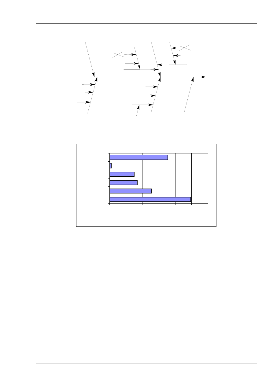
Quantifying Uncertainty

Example A2

QUAM:2000.1

Page 41

Figure A2.2: Cause and effect diagram for titration

c(NaOH)

P(KHP)

M(KHP)

V(T)

calibration

temperature

end-point

bias

m(KHP)

m(gross)

m(tare)

calibration

linearity

sensitivity

calibration

linearity

sensitivity

repeatability

V(T)

end-point

m(KHP)

Figure A2.3: Contributions to Titration uncertainty

u(y,x

) (mmol l

-1

)

0.02

0.04

0.06

0.08

0.1

0.12

c(NaOH)

Repeatability

m(KHP)

P(KHP)

M(KHP)

V(T)

The values of

u(y,x

)=(

∂

u(x

) are taken from Table A2.3

Quantifying Uncertainty

Example A2

QUAM:2000.1

Page 42

Example A2: Standardising a sodium hydroxide solution. Detailed discussion

A2.1 Introduction

This second introductory example discusses an
experiment to determine the concentration of a
solution of sodium hydroxide (NaOH). The
NaOH is titrated against the titrimetric standard
potassium hydrogen phthalate (KHP). It is
assumed that the NaOH concentration is known to
be of the order of 0.1 mol l

–1

. The end-point of the

titration is determined by an automatic titration
system using a combined pH-electrode to measure
the shape of the pH-curve. The functional
composition of the titrimetric standard potassium
hydrogen phthalate (KHP), which is the number
of free protons in relation to the overall number of
molecules, provides traceability of the
concentration of the NaOH solution to the SI
system.

A2.2 Step 1: Specification

The aim of the first step is to describe the
measurement procedure. This description consists
of a listing of the measurement steps and a
mathematical statement of the measurand and the
parameters upon which it depends.

Procedure:

The measurement sequence to standardise the
NaOH solution has the following stages.

Figure A2.4: Standardisation of a solution of

sodium hydroxide

Weighing KHP

Preparing NaOH

Titration

RESULT

The separate stages are:

The primary standard potassium hydrogen
phthalate (KHP) is dried according to the
supplier’s instructions. The instructions are
given in the supplier's catalogue, which also
states the purity of the titrimetric standard
and its uncertainty. A titration volume of
approximately 19 ml of 0.1 mol l

-1

solution of

NaOH entails weighing out an amount as
close as possible to

388

1000

2212

204

The weighing is carried out on a balance with
a last digit of 0.1 mg.

ii) A 0.1 mol l

-1

solution of sodium hydroxide is

prepared. In order to prepare 1 l of solution,
it is necessary to weigh out

≈

4 g NaOH.

However, since the concentration of the
NaOH solution is to be determined by assay
against the primary standard KHP and not by
direct calculation, no information on the
uncertainty sources connected with the
molecular weight or the mass of NaOH taken
is required.

iii) The weighed quantity of the titrimetric

standard KHP is dissolved with

≈

50 ml of

ion-free water and then titrated using the
NaOH solution. An automatic titration
system controls the addition of NaOH and
records the pH-curve. It also determines the
end-point of the titration from the shape of
the recorded curve.

Calculation:

The measurand is the concentration of the NaOH
solution, which depends on the mass of KHP, its
purity, its molecular weight and the volume of
NaOH at the end-point of the titration

]

mol

[

1000

−

⋅

KHP

NaOH

where

NaOH

:concentration of the NaOH solution
[mol l

–1

]

1000

:conversion factor [ml] to [l]

KHP

:mass of the titrimetric standard KHP [g]

Quantifying Uncertainty

Example A2

QUAM:2000.1

Page 43

KHP

:purity of the titrimetric standard given
as mass fraction

KHP

:molar mass of KHP [g mol

–1

]

:titration volume of NaOH solution [ml]

A2.3 Step 2: Identifying and analysing

uncertainty sources

The aim of this step is to identify all major
uncertainty sources and to understand their effect
on the measurand and its uncertainty. This has
been shown to be one of the most difficult step in
evaluating the uncertainty of analytical
measurements, because there is a risk of

neglecting uncertainty sources on the one hand
and an the other of double-counting them. The
use of a cause and effect diagram (Appendix D) is
one possible way to help prevent this happening.
The first step in preparing the diagram is to draw
the four parameters of the equation of the
measurand as the main branches.

Afterwards, each step of the method is considered

and any further influence quantity is added as a
factor to the diagram working outwards from the
main effect. This is carried out for each branch
until effects become sufficiently remote, that is,
until effects on the result are negligible.

Mass m

KHP

Approximately 388 mg of KHP are weighed to
standardise the NaOH solution. The weighing
procedure is a weight by difference. This means
that a branch for the determination of the tare
(

tare

) and another branch for the gross weight

(

gross

) have to be drawn in the cause and effect

diagram. Each of the two weighings is subject to
run to run variability and the uncertainty of the
calibration of the balance. The calibration itself
has two possible uncertainty sources: the
sensitivity and the linearity of the calibration
function. If the weighing is done on the same
scale and over a small range of weight then the
sensitivity contribution can be neglected.

All these uncertainty sources are added into the
cause and effect diagram (see Figure A2.6).

Purity P

KHP

The purity of KHP is quoted in the supplier's
catalogue to be within the limits of 99.95% and
100.05%.

KHP

is therefore 1.0000 ±0.0005. There

is no other uncertainty source if the drying
procedure was performed according to the
suppliers specification.

Molar mass M

KHP

Potassium hydrogen phthalate (KHP) has the

c(NaOH)

m(KHP)

P(KHP)

M(KHP)

V(T)

Figure A2.5: First step in setting up a cause

and effect diagram

c(NaOH)

m(KHP)

P(KHP)

M(KHP)

V(T)

m(gross)

m(tare)

repeatability

calibration

linearity

sensitivity

calibration

linearity

sensitivity

Figure A2.6:Cause and effect diagram with added uncertainty sources

for the weighing procedure

Quantifying Uncertainty

Example A2

QUAM:2000.1

Page 44

empirical formula

The uncertainty in the molar mass of the
compound can be determined by combining the
uncertainty in the atomic weights of its
constituent elements. A table of atomic weights
including uncertainty estimates is published
biennially by IUPAC in the Journal of Pure and
Applied Chemistry. The molar mass can be
calculated directly from these; the cause and
effect diagram (Figure A2.7) omits the individual
atomic masses for clarity

Volume V

The titration is accomplished using a 20 ml piston
burette. The delivered volume of NaOH from the
piston burette is subject to the same three
uncertainty sources as the filling of the volumetric
flask in the previous example. These uncertainty
sources are the repeatability of the delivered
volume, the uncertainty of the calibration of that
volume and the uncertainty resulting from the
difference between the temperature in the
laboratory and that of the calibration of the piston
burette. In addition there is the contribution of the
end-point detection, which has two uncertainty
sources.

1. The repeatability of the end-point detection,

which is independent of the repeatability of
the volume delivery.

2. The possibility of a systematic difference

between the determined end-point and the
equivalence point (bias), due to carbonate

absorption during the titration and inaccuracy
in the mathematical evaluation of the end-
point from the titration curve.

These items are included in the cause and effect
diagram shown in Figure A2.7.

A2.4 Step 3: Quantifying uncertainty

components

In step 3, the uncertainty from each source
identified in step 2 has to be quantified and then
converted to a standard uncertainty.

All

experiments always include at least the
repeatability of the volume delivery of the piston
burette and the repeatability of the weighing
operation. Therefore it is reasonable to combine
all the repeatability contributions into one
contribution for the overall experiment and to use
the values from the method validation to quantify
its size, leading to the revised cause and effect
diagram in Figure A2.8.

The method validation shows a repeatability for
the titration experiment of 0.05%. This value can
be directly used for the calculation of the
combined standard uncertainty.

Mass m

KHP

The relevant weighings are:

container and KHP:

60.5450 g(observed)

container less KHP:

60.1562 g(observed)

KHP

0.3888 g(calculated)

Because of the combined repeatability term
identified above, there is no need to take into
account the weighing repeatability. Any

c(NaOH)

P(KHP)

M(KHP)

V(T)

repeatability

calibration

temperature

end-point

bias

repeatability

m(KHP)

m(gross)

m(tare)

repeatability

calibration

linearity

sensitivity

calibration

linearity

sensitivity

Figure A2.7: Cause and effect diagram (all sources)

Quantifying Uncertainty

Example A2

QUAM:2000.1

Page 45

systematic offset across the scale will also cancel.
The uncertainty therefore arises solely from the
balance linearity uncertainty.

Linearity: The calibration certificate of the

balance quotes ±0.15 mg for the linearity. This
value is the maximum difference between the
actual mass on the pan and the reading of the
scale. The balance manufacture's own
uncertainty evaluation recommends the use of
a rectangular distribution to convert the
linearity contribution to a standard uncertainty.

The balance linearity contribution is
accordingly

This contribution has to be counted twice,
once for the tare and once for the gross weight,
because each is an independent observation
and the linearity effects are not correlated.

This gives for the standard uncertainty

u(m

KHP

) of

the mass

KHP

, a value of

)

(

)

(

)

(

⇒

KHP

OTE

1: Buoyancy correction is not considered

because all weighing results are quoted on the
conventional basis for weighing in air [H.19].
The remaining uncertainties are too small to
consider. Note 1 in Appendix G refers.

OTE

2: There are other difficulties when weighing a

titrimetric standard. A temperature difference
of only 1 °C between the standard and the

balance causes a drift in the same order of
magnitude as the repeatability contribution.
The titrimetric standard has been completely
dried, but the weighing procedure is carried
out at a humidity of around 50 % relative
humidity, so adsorption of some moisture is
expected.

Purity P

KHP

is 1.0000±0.0005. The supplier gives no

further information concerning the uncertainty in
the catalogue. Therefore this uncertainty is taken
as having a rectangular distribution, so the
standard uncertainty

u(P

KHP

) is

00029

0005

Molar mass M

KHP

From the latest IUPAC table, the atomic weights
and listed uncertainties for the constituent
elements of KHP (C

K) are:

Element

Atomic
weight

Quoted
uncertainty

Standard
uncertainty

12.0107

0.0008

0.00046

1.00794

0.00007

0.000040

15.9994

0.0003

0.00017

39.0983

0.0001

0.000058

For each element, the standard uncertainty is
found by treating the IUPAC quoted uncertainty
as forming the bounds of a rectangular
distribution. The corresponding standard
uncertainty is therefore obtained by dividing

those values by 3 .

c(NaOH)

P(KHP)

M(KHP)

V(T)

calibration

temperature

end-point

bias

m(KHP)

m(gross)

m(tare)

calibration

linearity

sensitivity

calibration

linearity

sensitivity

repeatability

V(T)

end-point

m(KHP)

Figure A2.8: Cause and effect diagram (Repeatabilities combined)

Quantifying Uncertainty

Example A2

QUAM:2000.1

Page 46

The separate element contributions to the molar
mass, together with the uncertainty contribution
for each, are:

Calculation Result

Standard
uncertainty

12.0107

96.0856

0.0037

1.00794

5.0397

0.00020

15.9994

63.9976

0.00068

39.0983

0.000058

The uncertainty in each of these values is
calculated by multiplying the standard uncertainty
in the previous table by the number of atoms.

This gives a molar mass for KHP of

mol

2212

204

0983

9976

0397

0856

−

KHP

As this expression is a sum of independent values,
the standard uncertainty u(M

KHP

) is a simple

square root of the sum of the squares of the
contributions:

mol

0038

)

(

000058

00068

0002

0037

)

(

−

⇒

KHP

OTE

Since the element contributions to M

KHP

are

simply the sum of the single atom
contributions, it might be expected from the
general rule for combing uncertainty
contributions that the uncertainty for each
element contribution would be calculated from
the sum of squares of the single atom
contributions, that is, for carbon,

001

00037

)

(

. Recall,

however, that this rule applies only to
independent contributions, that is,
contributions from separate determinations of
the value. In this case, the total is obtained by
multiplying a single value by 8. Notice that the
contributions from different elements are
independent, and will therefore combine in the
usual way.

Volume V

1. Repeatability of the volume delivery: As

before, the repeatability has already been taken
into account via the combined repeatability
term for the experiment.

2. Calibration: The limits of accuracy of the

delivered volume are indicated by the
manufacturer as a ± figure. For a 20 ml piston
burette this number is typically ±0.03

ml.

Assuming a triangular distribution gives a

standard uncertainty of

012

Note: The ISO Guide (F.2.3.3) recommends

adoption of a triangular distribution if
there are reasons to expect values in the
centre of the range being more likely
than those near the bounds. For the
glassware in examples A1 and A2, a
triangular distribution has been assumed
(see the discussion under Volume
uncertainties in example A1).

3. Temperature: The uncertainty due to the lack

of temperature control is calculated in the
same way as in the previous example, but this
time taking a possible temperature variation of
±3 °C (with a 95% confidence). Again using
the coefficient of volume expansion for water
as 2.1

–4

°C

–1

gives a value of

006

−

Thus the standard uncertainty due to
incomplete temperature control is 0.006 ml.

OTE

When dealing with uncertainties arising from
incomplete control of environmental factors
such as temperature, it is essential to take
account of any correlation in the effects on
different intermediate values. In this example,
the dominant effect on the solution
temperature is taken as the differential heating
effects of different solutes, that is, the
solutions are not equilibrated to ambient
temperature. Temperature effects on each
solution concentration at STP are therefore
uncorrelated in this example, and are
consequently treated as independent
uncertainty contributions.

4. Bias of the end-point detection: The titration is

performed under a layer of Argon to exclude
any bias due to the absorption of CO

in the

titration solution. This approach follows the
principle that it is better to prevent any bias
than to correct for it. There are no other
indications that the end-point determined from
the shape of the pH-curve does not correspond
to the equivalence-point, because a strong acid
is titrated with a strong base. Therefore it is

Quantifying Uncertainty

Example A2

QUAM:2000.1

Page 47

assumed that the bias of the end-point
detection and its uncertainty are negligible.

is found to be 18.64 ml and combining the

remaining contributions to the uncertainty u(V

)

of the volume V

gives a value of

013

)

(

006

012

)

(

⇒

A2.5 Step 4: Calculating the combined

standard uncertainty

NaOH

is given by

]

mol

[

1000

−

⋅

KHP

NaOH

The values of the parameters in this equation,
their standard uncertainties and their relative
standard uncertainties are collected in Table A2.2

Using the values given above:

mol

10214

2212

204

3888

1000

−

NaOH

For a multiplicative expression (as above) the
standard uncertainties are used as follows:

)

(

)

(

)

(

)

(

)

(

)

(





























































KHP

NaOH

rep

00097

00070

000019

00029

00033

0005

)

(

⇒

NaOH

(

)

mol

00010

00097

−

⇒

NaOH

Spreadsheet software is used to simplify the
above calculation of the combined standard
uncertainty (see Appendix E.2). The spreadsheet
filled in with the appropriate values is shown as
Table A2.3, which appears with additional
explanation.

It is instructive to examine the relative
contributions of the different parameters. The
contributions can easily be visualised using a
histogram. Figure A2.9 shows the calculated
values |u(y,x

)| from Table A2.3.

The contribution of the uncertainty of the titration
volume V

is by far the largest followed by the

repeatability. The weighing procedure and the
purity of the titrimetric standard show the same
order of magnitude, whereas the uncertainty in the
molar mass is again nearly an order of magnitude
smaller.

Table A2.2: Values and uncertainties for titration

Description

Value x

Standard uncertainty

u(x)

Relative standard

uncertainty u(x)/x

rep

Repeatability

1.0

0.0005

KHP

Weight of KHP

0.3888 g

0.00013 g

0.00033

KHP

Purity of KHP

1.0

0.00029

KHP

Molar mass of KHP

204.2212 g mol

-1

0.0038 g mol

-1

0.000019

Volume of NaOH for KHP
titration

18.64 ml

0.013 ml

0.0007

Figure A2.9: Uncertainty contributions in

NaOH standardisation

u(y,x

) (mmol l

-1

)

0.02

0.04

0.06

0.08

0.1

0.12

c(NaOH)

Repeatability

m(KHP)

P(KHP)

M(KHP)

V(T)

Quantifying Uncertainty

Example A2

QUAM:2000.1

Page 48

A2.6 Step 5: Re-evaluate the significant

components

The contribution of V(T) is the largest one. The
volume of NaOH for titration of KHP (V(T)) itself
is affected by four influence quantities: the
repeatability of the volume delivery, the
calibration of the piston burette, the difference
between the operation and calibration temperature
of the burette and the repeatability of the end-
point detection. Checking the size of each
contribution, the calibration is by far the largest.
Therefore this contribution needs to be
investigated more thoroughly.

The standard uncertainty of the calibration of
V(T) was calculated from the data given by the
manufacturer assuming a triangular distribution.
The influence of the choice of the shape of the
distribution is shown in Table A2.4.

According to the ISO Guide 4.3.9 Note 1:

“For a normal distribution with expectation

and standard deviation

, the interval

±3

encompasses approximately 99.73 percent of
the distribution. Thus, if the upper and lower
bounds a+ and a- define 99.73 percent limits

rather than 100 percent limits, and X

can be

assumed to be approximately normally
distributed rather than there being no specific
knowledge about X

[between the bounds], then

) = a

/9. By comparison, the variance of a

symmetric rectangular distribution of the half-
width a is a

/3 ... and that of a symmetric

triangular distribution of the half-width a is a

... The magnitudes of the variances of the three
distributions are surprisingly similar in view of
the differences in the assumptions upon which
they are based.”

Thus the choice of the distribution function of
this influence quantity has little effect on the
value of the combined standard uncertainty
(u

NaOH

)) and it is adequate to assume that it is

triangular.

Table A2.3: Spreadsheet calculation of titration uncertainty

Rep

m(KHP)

P(KHP)

M(KHP)

V(T)

Value

1.0

0.3888

1.0

204.2212

18.64

Uncertainty 0.0005

0.00013

0.00029

0.0038

0.013

rep

1.0

1.0005

1.0

m(KHP)

0.3888

0.38893

0.3888

P(KHP)

1.0

1.00029

1.0

M(KHP)

204.2212

204.2250

204.2212

V(T)

18.64

18.653

c(NaOH)

0.102136

0.102187

0.102170

0.102166

0.102134

0.102065

u(y,x

)

0.000051

0.000034

0.000030

-0.000002

-0.000071

u(y)

, u(y,x

)

9.72E-9

2.62E-9

1.16E-9

9E-10

4E-12

5.041E-9

u(c(NaOH)) 0.000099

The values of the parameters are given in the second row from C2 to G2. Their standard uncertainties are entered in the
row below (C3-G3). The spreadsheet copies the values from C2-G2 into the second column from B5 to B9. The result
(c(NaOH)) using these values is given in B11. C5 shows the value of the repeatability from C2 plus its uncertainty given
in C3. The result of the calculation using the values C5-C9 is given in C11. The columns D and G follow a similar
procedure. The values shown in the row 12 (C12-G12) are the differences of the row (C11-G11) minus the value given
in B11. In row 13 (C13-G13) the values of row 12 (C12-G12) are squared and summed to give the value shown in B13.
B15 gives the combined standard uncertainty, which is the square root of B13.

Quantifying Uncertainty

Example A2

QUAM:2000.1

Page 49

The expanded uncertainty U(c

NaOH

) is obtained by

multiplying the combined standard uncertainty by
a coverage factor of 2.

mol

0002

00010

)

(

−

NaOH

Thus the concentration of the NaOH solution is
(

0.1021 ±0.0002) mol l

–1

Table A2.4: Effect of different distribution assumptions

Distribution

factor

u(V(T;cal))

(ml)

u(V(T))

(ml)

NaOH

)

Rectangular

0.017

0.019

0.00011 mol l

-1

Triangular

0.012

0.015

0.00009 mol l

-1

Normal

Note 1

0.010

0.013

0.000085 mol l

-1

Note 1: The factor of 9 arises from the factor of 3 in Note 1 of ISO Guide
4.3.9 (see page 48 for details).

Quantifying Uncertainty

Example A3

QUAM:2000.1

Page 50

Example A3: An Acid/Base Titration

Summary

Goal

A solution of hydrochloric acid (HCl) is
standardised against a solution of sodium
hydroxide (NaOH) with known content.

Measurement procedure

A solution of hydrochloric acid (HCl) is titrated
against a solution of sodium hydroxide (NaOH),
which has been standardised against the
titrimetric standard potassium hydrogen phthalate
(KHP), to determine its concentration. The stages
of the procedure are shown in Figure A3.1.

Measurand:

HCl

KHP

HCl

⋅

1000

[mol l

-1

]

where the symbols are as given in Table A3.1 and
the value of 1000 is a conversion factor from ml
to litres.

Identification of the uncertainty sources:

The relevant uncertainty sources are shown in
Figure A3.2.

Quantification of the uncertainty components

The final uncertainty is estimated as
0.00016 mol l

-1

. Table A3.1 summarises the

values and their uncertainties; Figure A3.3 shows
the values diagrammatically.

Figure A3.1: Titration procedure

Weighing KHP

Titrate KHP

with NaOH

Titrate KHP

with NaOH

Take aliquot

of HCl

Take aliquot

of HCl

Titrate HCl
with NaOH

RESULT

Figure A3.2: Cause and Effect diagram for acid-base titration

V(T2)

Calibration

Temperature

m(KHP)

V(T2)

end-point V(T2)

V(T1)

end-point V(T1)

V(HCl)

End point

Temperature

Calibration

Bias

Calibration

sensitivity

linearity

sensitivity

linearity

same balance

m(gross)

c(HCl)

m(KHP)

P(KHP)

M(KHP)

V(HCl)

V(T1)

Bias

End point

Temperature

Calibration

m(tare)

Repeatability

Quantifying Uncertainty

Example A3

QUAM:2000.1

Page 51

Table A3.1: Acid-base Titration values and uncertainties

Description

Value x

Standard

uncertainty u(x)

Relative standard

uncertainty u(x)/x

rep

Repeatability

0.001

KHP

Weight of KHP

0.3888 g

0.00013 g

0.00033

KHP

Purity of KHP

1.0

0.00029

Volume of NaOH for HCl titration

14.89 ml

0.015 ml

0.0010

Volume of NaOH for KHP titration

18.64 ml

0.016 ml

0.00086

KHP

Molar mass of KHP

204.2212 g mol

-1

0.0038 g mol

-1

0.000019

HCl

HCl aliquot for NaOH titration

15 ml

0.011 ml

0.00073

HCl

HCl solution concentration

0.10139 mol l

-1

0.00016 mol l

-1

0.0016

Figure A3.3: Uncertainty contributions in acid-base titration

u(y,x

) (mmol l

-1

)

0.05

0.1

0.15

0.2

c(HCl)

Repeatability

m(KHP)

P(KHP)

V(T2)

V(T1)

M(KHP)

V(HCl)

The values of u(y,x

)=(

∂

).u(x

) are taken from Table A3.3.

Quantifying Uncertainty

Example A3

QUAM:2000.1

Page 52

Example A3: An acid/base titration. Detailed discussion

A3.1 Introduction

This example discusses a sequence of
experiments to determine the concentration of a
solution of hydrochloric acid (HCl). In addition, a
number of special aspects of the titration
technique are highlighted. The HCl is titrated
against solution of sodium hydroxide (NaOH),
which was freshly standardised with potassium
hydrogen phthalate (KHP). As in the previous
example (A2) it is assumed that the HCl
concentration is known to be of the order of
0.1 mol l

–1

and that the end-point of the titration

is determined by an automatic titration system
using the shape of the pH-curve. This evaluation
gives the measurement uncertainty in terms of the
SI units of measurement.

A3.2 Step 1: Specification

A detailed description of the measurement
procedure is given in the first step. It
compromises a listing of the measurement steps
and a mathematical statement of the measurand.

Procedure

The determination of the concentration of the
HCl solution consists of the following stages (See
also Figure A3.4):

The titrimetric standard potassium hydrogen
phthalate (KHP) is dried to ensure the purity
quoted in the supplier's certificate.
Approximately 0.388 g of the dried standard
is then weighed to achieve a titration volume
of 19 ml NaOH.

ii) The KHP titrimetric standard is dissolved

with

≈

50 ml of ion free water and then

titrated using the NaOH solution. A titration
system controls automatically the addition of
NaOH and samples the pH-curve. The end-
point is evaluated from the shape of the
recorded curve.

iii) 15 ml of the HCl solution is transferred by

means of a volumetric pipette. The HCl
solution is diluted with de-ionised water to
give

≈

50 ml solution in the titration vessel.

iv) The same automatic titrator performs the

measurement of HCl solution.

Weighing KHP

Titrate KHP

with NaOH

Titrate KHP

with NaOH

Take aliquot

of HCl

Take aliquot

of HCl

Titrate HCl
with NaOH

RESULT

Figure A3.4: Determination of the

concentration of a HCl solution

Calculation:

The measurand is the concentration of the HCl
solution, c

HCl

. It depends on the mass of KHP, its

purity, its molecular weight, the volumes of
NaOH at the end-point of the two titrations and
the aliquot of HCl.:

]

mol

[

1000

−

⋅

HCl

KHP

HCl

where

HCl

:concentration of the HCl solution
[mol l

-1

]

1000

:conversion factor [ml] to [l]

KHP

:mass of KHP taken [g]

KHP

:purity of KHP given as mass fraction

:volume of NaOH solution to titrate HCl
[ml]

:volume of NaOH solution to titrate KHP
[ml]

KHP

: molar mass of KHP [g mol

–1

]

HCl

:volume of HCl titrated with NaOH
solution [ml]

Quantifying Uncertainty

Example A3

QUAM:2000.1

Page 53

A3.3 Step 2: Identifying and analysing

uncertainty sources

The different uncertainty sources and their
influence on the measurand are best analysed by
visualising them first in a cause and effect
diagram (Figure A3.5).

Because a repeatability estimate is available from
validation studies for the procedure as a whole,
there is no need to consider all the repeatability
contributions individually. They are therefore
grouped into one contribution (shown in the
revised cause and effect diagram in Figure A3.5).

The influences on the parameters V

, V

, m

KHP

and M

KHP

have been discussed extensively in

the previous example, therefore only the new
influence quantities of V

HCl

will be dealt with in

more detail in this section.

Volume V

HCl

15 ml of the investigated HCl solution is to be
transferred by means of a volumetric pipette. The
delivered volume of the HCl from the pipette is
subject to the same three sources of uncertainty as
all the volumetric measuring devices.

1. The variability or repeatability of the delivered

volume

2. The uncertainty in the stated volume of the

pipette

3. The solution temperature differing from the

calibration temperature of the pipette.

A3.4 Step 3: Quantifying uncertainty

components

The goal of this step is to quantify each
uncertainty source analysed in step

2. The

quantification of the branches or rather of the
different components was described in detail in
the previous two examples. Therefore only a
summary for each of the different contributions
will be given.

repeatability

The method validation shows a repeatability for
the determination of 0.1% (as %rsd). This value
can be used directly for the calculation of the
combined standard uncertainty associated with
the different repeatability terms.

Mass m

KHP

Calibration/linearity: The balance manufacturer

quotes ±0.15 mg for the linearity contribution.
This value represents the maximum difference
between the actual mass on the pan and the
reading of the scale. The linearity contribution
is assumed to show a rectangular distribution
and is converted to a standard uncertainty:

087

The contribution for the linearity has to be
accounted for twice, once for the tare and once
for the gross mass, leading to an uncertainty
u(m

KHP

) of

)

(

)

087

(

)

(

⇒

KHP

OTE

1: The contribution is applied twice because no

assumptions are made about the form of the
non-linearity. The non-linearity is accordingly
treated as a systematic effect on each
weighing, which varies randomly in
magnitude across the measurement range.

Figure A3.5: Final cause and effect diagram

V(T2)

Calibration

Temperature

m(KHP)

V(T2)

end-point V(T2)

V(T1)

end-point V(T1)

V(HCl)

End point

Temperature

Calibration

Bias

Calibration

sensitivity

linearity

sensitivity

linearity

same balance

m(gross)

c(HCl)

m(KHP)

P(KHP)

M(KHP)

V(HCl)

V(T1)

Bias

End point

Temperature

Calibration

m(tare)

Repeatability

Quantifying Uncertainty

Example A3

QUAM:2000.1

Page 54

OTE

2: Buoyancy correction is not considered

because all weighing results are quoted on the
conventional basis for weighing in air [H.19].
The remaining uncertainties are too small to
consider. Note 1 in Appendix G refers.

P(KHP)

P(KHP) is given in the supplier's certificate as
100% ±0.05%. The quoted uncertainty is taken as
a rectangular distribution, so the standard
uncertainty u(P

KHP

) is

00029

0005

)

(

KHP

(T2)

i) Calibration: Figure given by the manufacturer

(±0.03 ml) and approximated to a triangular

distribution

012

ii) Temperature: The possible temperature

variation is within the limits of ±4 °C and
approximated to a rectangular distribution

007

−

iii) Bias of the end-point detection: A bias

between the determined end-point and the
equivalence-point due to atmospheric CO

can

be prevented by performing the titration under
Argon. No uncertainty allowance is made.

is found to be 14.89 ml and combining the

two contributions to the uncertainty u(V

) of the

volume V

gives a value of

014

)

(

007

012

)

(

⇒

Volume V

All contributions except the one for the
temperature are the same as for V

i) Calibration:

012

ii) Temperature: The approximate volume for the

titration of 0.3888 g KHP is 19 ml NaOH,
therefore its uncertainty contribution is

009

−

iii) Bias: Negligible

is found to be 18.64 ml with a standard

uncertainty u(V

) of

015

)

(

009

012

)

(

⇒

Molar mass M

KHP

Atomic weights and listed uncertainties (from
current IUPAC tables) for the constituent
elements of KHP (C

K) are:

Element

Atomic

weight

Quoted

uncertainty

Standard

uncertainty

12.0107

0.0008

0.00046

1.00794

0.00007

0.000040

15.9994

0.0003

0.00017

39.0983

0.0001

0.000058

those values by 3 .

The molar mass M

KHP

for KHP and its uncertainty

KHP

)are, respectively:

mol

2212

204

0983

9994

00794

0107

−

KHP

mol

0038

)

(

000058

)

00017

(

)

00004

(

)

00046

(

)

(

−

⇒

KHP

OTE

The single atom contributions are not
independent. The uncertainty for the atom
contribution is therefore calculated by
multiplying the standard uncertainty of the
atomic weight by the number of atoms.

Volume V

HCl

i) Calibration: Uncertainty stated by the

manufacturer for a 15 ml pipette as ±0.02 ml
and approximated with a triangular

distribution:

008

ii) Temperature: The temperature of the

laboratory is within the limits of ±4 °C. Using
a rectangular temperature distribution gives a

standard uncertainty of

−

= 0.007 ml.

Combining these contributions gives

011

)

(

007

008

0037

)

(

⇒

HCl

Quantifying Uncertainty

Example A3

QUAM:2000.1

Page 55

A3.5 Step 4: Calculating the combined

standard uncertainty

HCl

is given by

HCl

KHP

HCl

⋅

1000

OTE

: The repeatability estimate is, in this example,

treated as a relative effect; the complete
model equation is therefore

rep

HCl

KHP

HCl

⋅

1000

All the intermediate values of the two step
experiment and their standard uncertainties are
collected in Table A3.2. Using these values:

mol

10139

2212

204

3888

1000

HCl

The uncertainties associated with each
component are combined accordingly:

0018

001

00073

000019

00080

00094

00029

00031

)

(

)

(

)

(

)

(

)

(

)

(

)

(

)

(









































































rep

HCl

KHP

HCl

mol

00018

0018

)

(

−

⇒

HCl

A spreadsheet method (see Appendix E) can be
used to simplify the above calculation of the

combined standard uncertainty. The spreadsheet
filled in with the appropriate values is shown in
Table A3.3, with an explanation.

The sizes of the different contributions can be
compared using a histogram. Figure A3.6 shows
the values of the contributions |u(y,x

)| from

Table A3.3.

Figure A3.6: Uncertainties in acid-base

titration

u(y,x

) (mmol l

-1

)

0.05

0.1

0.15

0.2

c(HCl)

Repeatability

m(KHP)

P(KHP)

V(T2)

V(T1)

M(KHP)

V(HCl)

The expanded uncertainty U(c

HCl

) is calculated by

multiplying the combined standard uncertainty by
a coverage factor of 2:

-1

mol

0004

00018

)

(

HCl

The concentration of the HCl solution is

(0.1014 ±0.0004) mol l

–1

Table A3.2: Acid-base Titration values and uncertainties (2-step procedure)

Description

Value x

Standard

Uncertainty u(x)

Relative standard

uncertainty u(x)/x

rep

Repeatability

0.001

KHP

Mass of KHP

0.3888 g

0.00012 g

0.00031

KHP

Purity of KHP

1.0

0.00029

Volume of NaOH for HCl titration

14.89 ml

0.014 ml

0.00094

Volume of NaOH for KHP titration

18.64 ml

0.015 ml

0.00080

KHP

Molar mass of KHP

204.2212 g mol

-1

0.0038 g mol

-1

0.000019

HCl

HCl aliquot for NaOH titration

15 ml

0.011 ml

0.00073

Quantifying Uncertainty

Example A3

QUAM:2000.1

Page 56

A3.6 Special aspects of the titration example

Three special aspects of the titration experiment
will be dealt with in this second part of the
example. It is interesting to see what effect
changes in the experimental set up or in the
implementation of the titration would have on the
final result and its combined standard uncertainty.

Influence of a mean room temperature of 25

For routine analysis, analytical chemists rarely
correct for the systematic effect of the
temperature in the laboratory on the volume. This
question considers the uncertainty introduced by
the corrections required.

The volumetric measuring devices are calibrated
at a temperature of 20

C. But rarely does any

analytical laboratory have a temperature
controller to keep the room temperature that
level. For illustration, consider correction for a
mean room temperature of 25

The final analytical result is calculated using the
corrected volumes and not the calibrated volumes
at 20

C. A volume is corrected for the

temperature effect according to

)]

(

[

−

where

:actual volume at the mean temperature T

:volume calibrated at 20

:expansion coefficient of an aqueous

solution [

–1

]

:observed temperature in the laboratory

[

The equation of the measurand has to be
rewritten:

HCl

KHP

HCl

1000

⋅

Table A3.3: Acid-base Titration – spreadsheet calculation of uncertainty

rep

m(KHP)

P(KHP)

V(T2)

V(T1)

M(KHP)

V(HCl)

value

1.0

0.3888

1.0

14.89

18.64

204.2212

uncertainty

0.001

0.00012

0.00029

0.014

0.015

0.0038

0.011

rep

1.0

1.001

1.0

m(KHP) 0.3888

0.3888

0.38892

0.3888

P(KHP)

1.0

1.00029

1.0

V(T2)

14.89

14.904

14.89

V(T1)

18.64

18.655

18.64

10 M(KHP) 204.2212 204.2212

204.2212

204.2250

204.2212

V(HCl)

15.011

c(HCl)

0.101387 0.101489

0.101418

0.101417

0.101482

0.101306

0.101385

0.101313

u(y, x

)

0.000101

0.000031

0.000029

0.000095

-0.000082 -0.0000019 -0.000074

u(y)

u(y, x

)

3.34E-8

1.03E-8

9.79E-10

8.64E-10

9.09E-9

6.65E-9

3.56E-12

5.52E-9

17 u(c(HCl)) 0.00018

The values of the parameters are given in the second row from C2 to I2. Their standard uncertainties are entered in the row
below (C3-I3). The spreadsheet copies the values from C2-I2 into the second column from B5 to B11. The result (c(HCl))
using these values is given in B13. The C5 shows the value of the repeatability from C2 plus its uncertainty given in C3.
The result of the calculation using the values C5-C11 is given in C13. The columns D to I follow a similar procedure. The
values shown in the row 14 (C14-I14) are the differences of the row (C13-H13) minus the value given in B13. In row 15
(C15-I15) the values of row 14 (C14-I14) are squared and summed to give the value shown in B15. B17 gives the combined
standard uncertainty, which is the square root of B15.

Quantifying Uncertainty

Example A3

QUAM:2000.1

Page 57

Including the temperature correction terms gives:













−

⋅

−













⋅

)]

(

[

)]

(

[

)]

(

[

1000

HCl

KHP

HCl

KHP

HCl

This expression can be simplified by assuming
that the mean temperature T and the expansion
coefficient of an aqueous solution

are the same

for all three volumes













−

⋅













⋅

)]

(

[

1000

HCl

KHP

HCl

This gives a slightly different result for the HCl
concentration at 20

mol

10149

)]

(

[

2236

204

3888

1000

−

HCl

The figure is still within the range given by the
combined standard uncertainty of the result at a
mean temperature of 20

C, so the result is not

significantly affected. Nor does the change affect
the evaluation of the combined standard
uncertainty, because a temperature variation of
±4

C at the mean room temperature of 25

C is

still assumed.

Visual end-point detection

A bias is introduced if the indicator
phenolphthalein is used for visual end-point
detection, instead of an automatic titration system
extracting the equivalence-point from the pH
curve. The change of colour from transparent to
red/purple occurs between pH 8.2 and 9.8 leading
to an excess volume, introducing a bias compared
to the end-point detection employing a pH meter.
Investigations have shown that the excess volume
is around 0.05 ml with a standard uncertainty for
the visual detection of the end-point of
approximately 0.03 ml. The bias arising from the
excess volume has to be considered in the
calculation of the final result. The actual volume
for the visual end-point detection is given by

Excess

Ind

;

where

Ind

;

:volume from a visual end-point detection

:volume at the equivalence-point

Excess

:excess volume needed to change the colour

of phenolphthalein

The volume correction quoted above leads to the
following changes in the equation of the
measurand

HCl

Excess

Ind

KHP

Excess

Ind

KHP

HCl

⋅

−

⋅

−

⋅

)

(

)

(

1000

;

The standard uncertainties u(V

) and u(V

) have

to be recalculated using the standard uncertainty
of the visual end-point detection as the
uncertainty component of the repeatability of the
end-point detection.

034

009

012

004

)

(

)

(

;

−

Excess

Ind

033

007

012

004

)

(

)

(

;

−

Excess

Ind

The combined standard uncertainty

mol

0003

)

(

−

HCl

is considerable larger than before.

Triple determination to obtain the final result

The two step experiment is performed three times
to obtain the final result. The triple determination
is expected to reduce the contribution from
repeatability, and hence reduce the overall
uncertainty.

As shown in the first part of this example, all the
run to run variations are combined to one single
component, which represents the overall
experimental repeatability as shown in the in the
cause and effect diagram (Figure A3.5).

The uncertainty components are quantified in the
following way:

Mass m

KHP

Linearity:

087

)

(

⇒

KHP

Purity P

KHP

Purity:

00029

0005

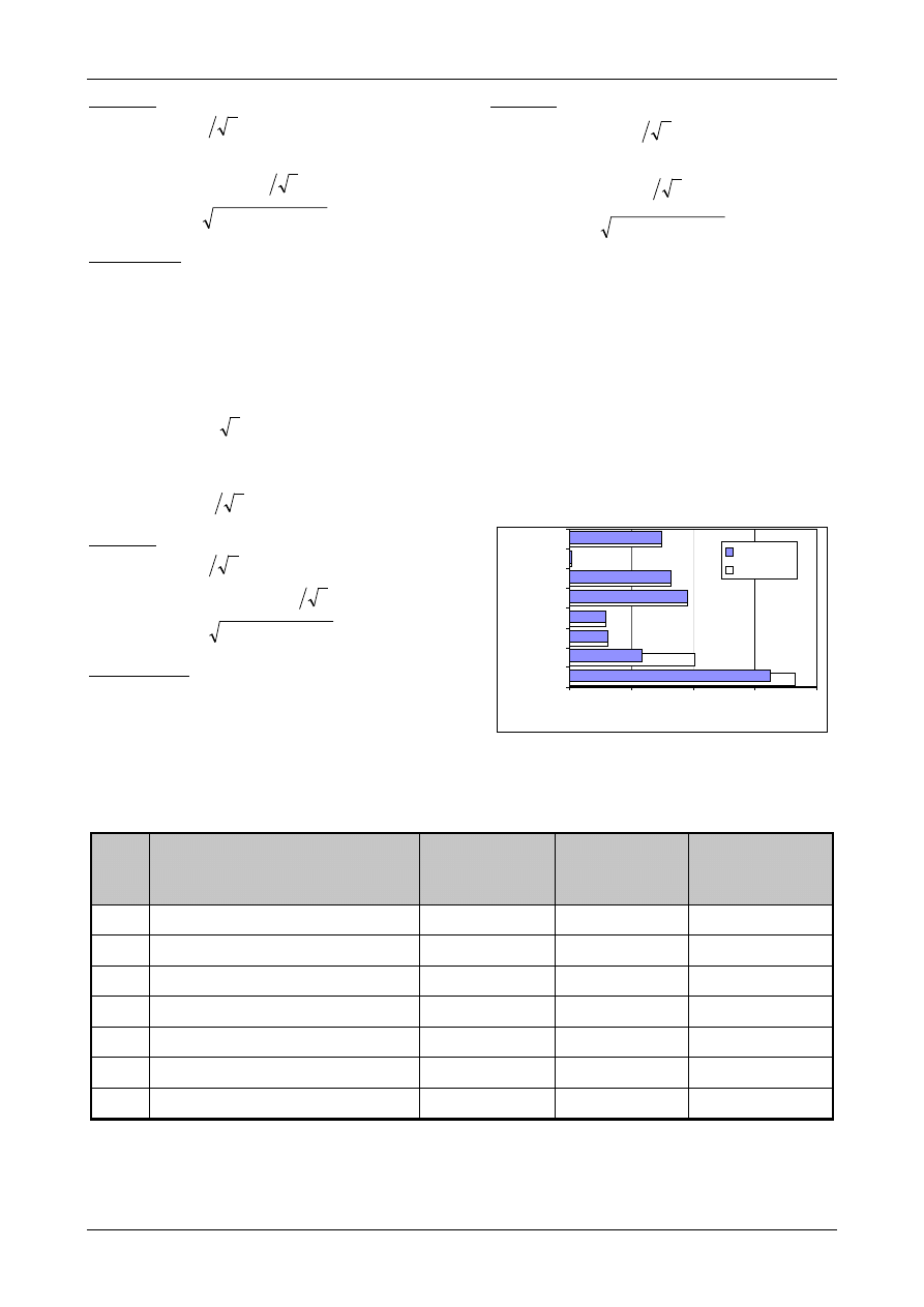
Quantifying Uncertainty

Example A3

QUAM:2000.1

Page 58

Volume V

calibration:

012

temperature:

007

−

( )

014

007

012

⇒

Repeatability

The quality log of the triple determination shows
a mean long term standard deviation of the
experiment of 0.001 (as RSD). It is not
recommended to use the actual standard deviation
obtained from the three determinations because
this value has itself an uncertainty of 52%. The
standard deviation of 0.001 is divided by the

square root of 3 to obtain the standard
uncertainty of the triple determination (three
independent measurements)

00058

001

Rep

(as RSD)

Volume V

HCl

calibration:

008

temperature:

007

−

(

)

007

008

⇒

HCl

Molar mass M

KHP

(

)

mol

0038

−

KHP

Volume V

calibration:

temperature:

009

−

( )

015

009

012

⇒

All the values of the uncertainty components are
summarised in Table A3.4. The combined
standard uncertainty is 0.00016 mol l

–1

, which is a

very modest reduction due to the triple
determination. The comparison of the uncertainty
contributions in the histogram, shown in Figure
A3.7, highlights some of the reasons for that
result. Though the repeatability contribution is
much reduced, the volumetric uncertainty
contributions remain, limiting the improvement.

Figure A3.7: Replicated Acid-base Titration

values and uncertainties

u(y,x

) (mmol l

-1

)

0.05

0.1

0.15

0.2

c(HCl)

Repeatability

m(KHP)

P(KHP)

V(T2)

V(T1)

M(KHP)

V(HCl)

Replicated

Single run

Table A3.4: Replicated Acid-base Titration values and uncertainties

Description

Value x

Standard

Uncertainty

u(x)

Relative Standard

Uncertainty

u(x)/x

Rep

Repeatability of the determination

1.0

0.00058

KHP

Mass of KHP

0.3888 g

0.00013 g

0.00033

KHP

Purity of KHP

1.0

0.00029

Volume of NaOH for HCl titration

14.90 ml

0.014 ml

0.00094

Volume of NaOH for KHP titration

18.65 ml

0.015 ml

0.0008

KHP

Molar mass of KHP

204.2212 g mol

-1

0.0038 g mol

-1

0.000019

HCl

HCl aliquot for NaOH titration

15 ml

0.01 ml

0.00067

Quantifying Uncertainty

Example A4

QUAM:2000.1

Page 59

Example A4: Uncertainty Estimation from In-House Validation Studies.

Determination of Organophosphorus Pesticides in Bread.

Summary

Goal

The amount of an organophosphorus pesticide
residue in bread is determined employing an
extraction and a GC procedure.

Measurement procedure

The stages needed to determine the amount of
organophosphorus pesticide residue are shown in
Figure A4.1

Measurand:

hom

sample

ref

Rec

⋅

mg kg

-1

where

:Level of pesticide in the sample
[mg kg

-1

]

:Peak intensity of the sample extract

ref

:Mass concentration of the reference
standard [

g ml

-1

]

:Final volume of the extract [ml]

ref

:Peak intensity of the reference standard

Rec

:Recovery

sample

:Mass of the investigated sub-sample [g]

hom

:Correction factor for sample
inhomogeneity

Identification of the uncertainty sources:

The relevant uncertainty sources are shown in the
cause and effect diagram in Figure A4.2.

Quantification of the uncertainty components:

Based on in-house validation data, the three major
contributions are listed in Table A4.1 and shown
diagrammatically in Figure A4.3 (values are from
Table A4.5).

Figure A4.1: Organophosphorus pesticides

analysis

RESULT

Homogenise

Extraction

Clean-up

‘Bulk up’

Determination

Prepare

calibration

standard

Prepare

calibration

standard

Calibration

Table A4.1: Uncertainties in pesticide analysis

Description

Value x

Standard

uncertainty u(x)

Relative standard

uncertainty u(x)/x

Comments

Repeatability(1)

1.0

0.27

Based on duplicate tests of
different types of samples

Bias (Rec) (2)

0.9

0.043

0.048

Spiked samples

Other sources (3)

(Homogeneity)

1.0

0.2

Estimation based on model
assumptions

- -

0.34

Relative standard uncertainty

Quantifying Uncertainty

Example A4

QUAM:2000.1

Page 60

Figure A4.2: Uncertainty sources in pesticide analysis

P(op)

I(op)

c(ref)

V(op)

m(sample)

I(ref)

V(op)

Calibration

Temperature

dilution

Calibration

V(ref)

Calibration

Temperature

m(ref)

Calibration

m(ref)

Purity (ref)

I(op)

Calibration

Recovery

m(gross)

I(ref)

Calibration

Linearity

m(tare)

m(sample)

Calibration

Linearity

F(hom)

Repeatability

Linearity

Figure A4.3: Uncertainties in pesticide analysis

u(y,x

) (mg kg

-1

)

0.1

0.2

0.3

0.4

P(op)

R epeatability

Bias

Hom ogeneity

The values of u(y,x

)=(

∂

).u(x

) are taken from Table A4.5

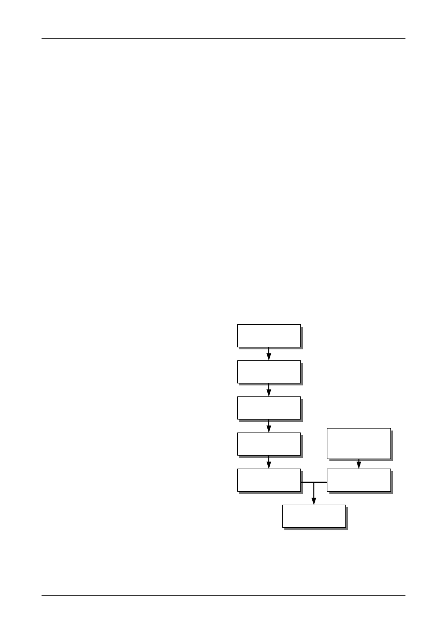
Quantifying Uncertainty

Example A4

QUAM:2000.1

Page 61

Example A4: Determination of organophosphorus pesticides in bread. Detailed

discussion.

A4.1 Introduction

This example illustrates the way in which in-
house validation data can be used to quantify the
measurement uncertainty. The aim of the
measurement is to determine the amount of an
organophosphorus pesticides residue in bread.
The validation scheme and experiments establish
traceability by measurements on spiked samples.
It is assumed the uncertainty due to any difference
in response of the measurement to the spike and
the analyte in the sample is small compared with
the total uncertainty on the result.

A4.2 Step 1: Specification

The specification of the measurand for more
extensive analytical methods is best done by a
comprehensive description of the different stages
of the analytical method and by providing the
equation of the measurand.

Procedure

The measurement procedure is illustrated
schematically in Figure A4.4. The separate stages
are:

i) Homogenisation: The complete sample is

divided into small (approx. 2 cm) fragments,
a random selection is made of about 15 of
these, and the sub-sample homogenised.
Where extreme inhomogeneity is suspected
proportional sampling is used before
blending.

ii) Weighing of sub-sampling for analysis gives

mass m

sample

iii) Extraction: Quantitative extraction of the

analyte with organic solvent, decanting and
drying through a sodium sulphate columns,
and concentration of the extract using a
Kuderna-Danish apparatus.

iv) Liquid-liquid extraction:

v) Acetonitrile/hexane liquid partition, washing

the acetonitrile extract with hexane, drying
the hexane layer through sodium sulphate
column.

vi) Concentration of the washed extract by gas

blown-down of extract to near dryness.

vii) Dilution to standard volume V

(approx.

2 ml) in a 10 ml graduated tube.

viii) Measurement: Injection and GC

measurement of 5

l of sample extract to

give the peak intensity I

ix) Preparation of an approximately 5

g ml

-1

standard (actual mass concentration c

ref

x) GC calibration using the prepared standard

and injection and GC measurement of 5

l of

the standard to give a reference peak
intensity I

ref

Figure A4.4: Organophosphorus pesticides

analysis

RESULT

Homogenise

Extraction

Clean-up

‘Bulk up’

Determination

Prepare

calibration

standard

Prepare

calibration

standard

Calibration

Quantifying Uncertainty

Example A4

QUAM:2000.1

Page 62

Calculation

The mass concentration c

in the final sample is

given by

−

⋅

ref

and the estimate P

of the level of pesticide in the

bulk sample (in mg kg

-1

) is given by

−

⋅

sample

Rec

or, substituting for c

sample

ref

Rec

⋅

where

:Level of pesticide in the sample [mg kg

-1

]

:Peak intensity of the sample extract

ref

:Mass concentration of the reference
standard [

g ml

-1

]

:Final volume of the extract [ml]

ref

:Peak intensity of the reference standard

Rec

:Recovery

sample

:Mass of the investigated sub-sample [g]

Scope

The analytical method is applicable to a small
range of chemically similar pesticides at levels
between 0.01 and 2 mg kg

-1

with different kinds

of bread as matrix.

A4.3 Step 2: Identifying and analysing

uncertainty sources

The identification of all relevant uncertainty
sources for such a complex analytical procedure
is best done by drafting a cause and effect
diagram. The parameters in the equation of the
measurand are represented by the main branches
of the diagram. Further factors are added to the
diagram, considering each step in the analytical
procedure (A4.2), until the contributory factors
become sufficiently remote.

The sample inhomogeneity is not a parameter in
the original equation of the measurand, but it
appears to be a significant effect in the analytical
procedure. A new branch, F(hom), representing
the sample inhomogeneity is accordingly added to
the cause and effect diagram (Figure A4.5).

Finally, the uncertainty branch due to the
inhomogeneity of the sample has to be included in
the calculation of the measurand. To show the
effect of uncertainties arising from that source
clearly, it is useful to write

Figure A4.5: Cause and effect diagram with added main branch for sample inhomogeneity

P(op)

I(op)

c(ref)

V(op)

m(sample)

I(ref)

Precision

Calibration

Temperature

dilution

Precision

Calibration

V(ref)

Precision

Calibration

Temperature

Precision

Calibration

m(ref)

Purity(ref)

Precision

Calibration

Recovery

m(gross)

Precision

Calibration

Precision

Calibration

Linearity

Sensitivity

m(tare)

Precision

Calibration

Linearity

Sensitivity

F(hom)

Linearity

Quantifying Uncertainty

Example A4

QUAM:2000.1

Page 63

]

[

−

⋅

sample

ref

hom

Rec

where F

hom

is a correction factor assumed to be

unity in the original calculation. This makes it
clear that the uncertainties in the correction factor
must be included in the estimation of the overall
uncertainty. The final expression also shows how
the uncertainty will apply.

OTE

Correction factors: This approach is quite
general, and may be very valuable in
highlighting hidden assumptions. In principle,
every measurement has associated with it such
correction factors, which are normally
assumed unity. For example, the uncertainty in
c

can be expressed as a standard uncertainty

for c

, or as the standard uncertainty which

represents the uncertainty in a correction
factor. In the latter case, the value is
identically the uncertainty for c

expressed as

a relative standard deviation.

A4.4 Step 3: Quantifying uncertainty

components

In accordance with section 7.7., the quantification
of the different uncertainty components utilises
data from the in-house development and
validation studies:

•

The best available estimate of the overall run

to run variation of the analytical process.

•

The best possible estimation of the overall

bias (Rec) and its uncertainty.

•

Quantification of any uncertainties associated

with effects incompletely accounted for the
overall performance studies.

Some rearrangement the cause and effect diagram
is useful to make the relationship and coverage of
these input data clearer (Figure A4.6).

OTE

In normal use, samples are run in small
batches, each batch including a calibration set,
a recovery check sample to control bias and
random duplicate to check precision.
Corrective action is taken if these checks show
significant departures from the performance
found during validation. This basic QC fulfils
the main requirements for use of the validation
data in uncertainty estimation for routine
testing.

Having inserted the extra effect ‘Repeatability’
into the cause and effect diagram, the implied
model for calculating P

becomes

−

⋅

Rep

sample

ref

hom

Rec

Eq. A4.1

That is, the repeatability is treated as a
multiplicative factor F

Rep

like the homogeneity.

This form is chosen for convenience in
calculation, as will be seen below.

Figure A4.6: Cause and effect diagram after rearrangement to accommodate the data of the

validation study

P(op)

I(op)

c(ref)

V(op)

m(sample)

I(ref)

V(op)

Calibration

Temperature

dilution

Calibration

V(ref)

Calibration

Temperature

m(ref)

Calibration

m(ref)

Purity (ref)

I(op)

Calibration

Recovery

m(gross)

I(ref)

Calibration

Linearity

m(tare)

m(sample)

Calibration

Linearity

F(hom)

Repeatability

Linearity

Quantifying Uncertainty

Example A4

QUAM:2000.1

Page 64

The evaluation of the different effects is now
considered.

1. Precision study

The overall run to run variation (precision) of the
analytical procedure was performed with a
number of duplicate tests (same homogenised
sample, complete extraction/determination
procedure) for typical organophosphorus
pesticides found in different bread samples. The
results are collected in Table A4.2.

The normalised difference data (the difference
divided by the mean) provides a measure of the
overall run to run variability. To obtain the
estimated relative standard uncertainty for single
determinations, the standard deviation of the
normalised differences is taken and divided by

2 to correct from a standard deviation for

pairwise differences to the standard uncertainty
for the single values. This gives a value for the
standard uncertainty due to run to run variation of
the overall analytical process, including run to run
recovery variation but excluding homogeneity

effects, of

382

OTE

At first sight, it may seem that duplicate tests
provide insufficient degrees of freedom. But it

is not the goal to obtain very accurate numbers
for the precision of the analytical process for
one specific pesticide in one special kind of
bread. It is more important in this study to test
a wide variety of different materials and
sample levels, giving a representative
selection of typical organophosphorus
pesticides. This is done in the most efficient
way by duplicate tests on many materials,
providing (for the repeatability estimate)
approximately one degree of freedom for each
material studied in duplicate.

2. Bias study

The bias of the analytical procedure was
investigated during the in-house validation study
using spiked samples (homogenised samples were
split and one portion spiked). Table A4.3 collects
the results of a long term study of spiked samples
of various types.

The relevant line (marked with grey colour) is the
"bread" entry line, which shows a mean recovery
for forty-two samples of 90%, with a standard
deviation (s) of 28%. The standard uncertainty
was calculated as the standard deviation of the

mean

0432

)

(

Rec

A significance test is used to determine whether
the mean recovery is significantly different from

Table A4.2: Results of duplicate pesticide analysis

Residue

[mg kg

-1

]

[mg kg

-1

]

Mean

[mg kg

-1

]

Difference

D1-D2

Difference/

mean

Malathion

1.30

0.00

0.000

Malathion

1.30

0.90

1.10

0.40

0.364

Malathion

0.57

0.53

0.55

0.04

0.073

Malathion

0.16

0.26

0.21

-0.10

-0.476

Malathion

0.65

0.58

0.62

0.07

0.114

Pirimiphos Methyl

0.04

0.00

0.000

Chlorpyrifos Methyl

0.08

0.09

0.085

-0.01

-0.118

Pirimiphos Methyl

0.02

0.00

0.000

Chlorpyrifos Methyl

0.01

0.02

0.015

-0.01

-0.667

Pirimiphos Methyl

0.02

0.01

0.015

0.01

0.667

Chlorpyrifos Methyl

0.03

0.02

0.025

0.01

0.400

Chlorpyrifos Methyl

0.04

0.06

0.05

-0.02

-0.400

Pirimiphos Methyl

0.07

0.08

0.75

-0.10

-0.133

Chlorpyrifos Methyl

0.01

0.10

0.00

0.000

Pirimiphos Methyl

0.06

0.03

0.045

0.03

0.667

Quantifying Uncertainty

Example A4

QUAM:2000.1

Page 65

1.0. The test statistic t is calculated using the
following equation

(

)

315

0432

)

(

−

Rec

This value is compared with the 2-tailed critical
value t

crit

, for n–1 degrees of freedom at 95%

confidence (where n is the number of results used

to estimate Rec ). If t is greater or equal than the

critical value t

crit

than Rec is significantly

different from 1.

021

;

≅

≥

crit

In this example a correction factor (1/ Rec ) is

being applied and therefore Rec is explicitly
included in the calculation of the result.

3. Other sources of uncertainty

The cause and effect diagram in Figure A4.7
shows which other sources of uncertainty are (1)
adequately covered by the precision data, (2)
covered by the recovery data or (3) have to be
further examined and eventually considered in the
calculation of the measurement uncertainty.

All balances and the important volumetric
measuring devices are under regular control.
Precision and recovery studies take into account

the influence of the calibration of the different
volumetric measuring devices because during the
investigation various volumetric flasks and
pipettes have been used. The extensive variability
studies, which lasted for more than half a year,
also cover influences of the environmental
temperature on the result. This leaves only the
reference material purity, possible nonlinearity in
GC response (represented by the ‘calibration’
terms for I

ref

and I

in the diagram), and the

sample homogeneity as additional components
requiring study.

The purity of the reference standard is given by
the manufacturer as 99.53% ±0.06%. The purity
is potential an additional uncertainty source with

a standard uncertainty of

00035

0006

(Rectangular distribution). But the contribution is
so small (compared, for example, to the precision
estimate) that it is clearly safe to neglect this
contribution.

Linearity of response to the relevant
organophosphorus pesticides within the given
concentration range is established during
validation studies. In addition, with multi-level
studies of the kind indicated in Table A4.2 and
Table A4.3, nonlinearity would contribute to the
observed precision. No additional allowance is

Table A4.3: Results of pesticide recovery studies

Substrate

Residue

Type

Conc.
[mg kg

–1

]

Mean

[%]

Waste Oil

PCB

10.0

Butter

0.65

109

Compound Animal Feed I

0.325

100

Animal & Vegetable Fats I

0.33

102

Brassicas 1987

0.32

104

Bread

0.13

Rusks

0.13

Meat & Bone Feeds

0.325

Maize Gluten Feeds

0.325

Rape Feed I

0.325

Wheat Feed I

0.325

Soya Feed I

0.325

Barley Feed I

0.325

(1) The number of experiments carried out

(2) The mean and sample standard deviation s are given as percentage recoveries.

Quantifying Uncertainty

Example A4

QUAM:2000.1

Page 66

required. The in-house validation study has
proven that this is not the case.

The homogeneity of the bread sub-sample is the
last remaining other uncertainty source. No
literature data were available on the distribution
of trace organic components in bread products,
despite an extensive literature search (at first sight
this is surprising, but most food analysts attempt
homogenisation rather than evaluate
inhomogeneity separately). Nor was it practical to
measure homogeneity directly. The contribution
has therefore been estimated on the basis of the
sampling method used.

To aid the estimation, a number of feasible
pesticide residue distribution scenarios were
considered, and a simple binomial statistical
distribution used to calculate the standard
uncertainty for the total included in the analysed
sample (see section A4.6). The scenarios, and the
calculated relative standard uncertainties in the
amount of pesticide in the final sample, were:

! Scenario (a) Residue distributed on the top

surface only: 0.58.

! Scenario (b) Residue distributed evenly over

the surface only: 0.20.

! Scenario

through the sample, but reduced in
concentration by evaporative loss or
decomposition close to the surface: 0.05-0.10
(depending on the "surface layer" thickness).

Scenario (a) is specifically catered for by
proportional sampling or complete
homogenisation: It would arise in the case of
decorative additions (whole grains) added to one
surface. Scenario (b) is therefore considered the
likely worst case. Scenario (c) is considered the
most probable, but cannot be readily
distinguished from (b). On this basis, the value of
0.20 was chosen.

OTE

For more details on modelling inhomogeneity
see the last section of this example.

A4.5 Step 4: Calculating the combined

standard uncertainty

During the in-house validation study of the
analytical procedure the repeatability, the bias
and all other feasible uncertainty sources had
been thoroughly investigated. Their values and
uncertainties are collected in Table A4.4.

The relative values are combined because the
model (equation A4.1) is entirely multiplicative:

Figure A4.7: Evaluation of other sources of uncertainty

P(op)

I(op)

c(ref)

V(op)

m(sample)

I(ref)

V(op)

Calibration(2)

Temperature(2)

dilution

Calibration(2)

V(ref)

Calibration(2)

Temperature(2)

m(ref)

Calibration (2)

m(ref)

Purity(ref)

I(op)

Calibration(3)

Recovery(2)

m(gross)

I(ref)

Calibration(3)

Calibration(2)

Linearity

m(tare)

m(sample)

Calibration(2)

Linearity

F(hom)(3)

Repeatability(1)

Linearity

(1)

Repeatabilty (F

Rep

in equation A4.1) considered during the variability investigation of the analytical procedure.

(2)

Considered during the bias study of the analytical procedure.

(3)

To be considered during the evaluation of the other sources of uncertainty.

Quantifying Uncertainty

Example A4

QUAM:2000.1

Page 67

⇒

)

(

048

)

(

The spreadsheet for this case (Table A4.5) takes
the form shown in Table A4.5. Note that the
spreadsheet calculates an absolute value
uncertainty (0.377) for a nominal corrected result
of 1.1111, giving a value of 0.373/1.11=0.34.

The relative sizes of the three different
contributions can be compared by employing a
histogram. Figure A4.8 shows the values |u(y,x

taken from Table A4.5.

The repeatability is the largest contribution to the
measurement uncertainty. Since this component is
derived from the overall variability in the method,
further experiments would be needed to show
where improvements could be made. For
example, the uncertainty could be reduced
significantly by homogenising the whole loaf
before taking a sample.

The expanded uncertainty U(P

) is calculated by

multiplying the combined standard uncertainty
with a coverage factor of 2 to give:

)

(

Table A4.4: Uncertainties in pesticide analysis

Description

Value x

Standard

uncertainty u(x)

Relative standard

uncertainty u(x)

Remark

Repeatability(1)

1.0

0.27

Duplicate tests of different
types of samples

Bias (Rec) (2)

0.9

0.043

0.048

Spiked samples

Other sources (3)

(Homogeneity)

1.0

0.2

Estimations founded on model
assumptions

- -

0.34

Relative standard uncertainty

Figure A4.8: Uncertainties in pesticide analysis

u(y,x

) (mg kg

-1

)

0.1

0.2

0.3

0.4

P(op)

R epeatability

Bias

Hom ogeneity

The values of u(y,x

)=(

∂

).u(x

) are taken from Table A4.5

Quantifying Uncertainty

Example A4

QUAM:2000.1

Page 68

A4.6 Special aspect: Modelling inhomogeneity
for organophosphorus pesticide uncertainty

Assuming that all of the material of interest in a
sample can be extracted for analysis irrespective
of its state, the worst case for inhomogeneity is
the situation where some part or parts of a sample
contain all of the substance of interest. A more
general, but closely related, case is that in which
two levels, say L

and L

of the material are

present in different parts of the whole sample.
The effect of such inhomogeneity in the case of
random sub-sampling can be estimated using
binomial statistics. The values required are the
mean

and the standard deviation

of the

amount of material in n equal portions selected
randomly after separation.

These values are given by

(

)

⇒

⋅

(

)

−

⋅

[1]

(

) (

)

−

⋅

−

⋅

[2]

where l

and l

are the amount of substance in

portions from regions in the sample containing
total fraction L

and L

respectively, of the total

amount X, and p

and p

are the probabilities of

selecting portions from those regions (n must be
small compared to the total number of portions
from which the selection is made).

The figures shown above were calculated as
follows, assuming that a typical sample loaf is
approximately 24

cm, using a portion

size of

cm (total of 432 portions) and

assuming 15 such portions are selected at random
and homogenised.

Scenario (a)

The material is confined to a single large face (the
top) of the sample. L

is therefore zero as is l

;

and L

=1. Each portion including part of the top

surface will contain an amount l

of the material.

For the dimensions given, clearly one in six
(2/12) of the portions meets this criterion, p

Table A4.5: Uncertainties in pesticide analysis

Repeatability

Bias

Homogeneity

value

1.0

0.9

1.0

uncertainty

0.27

0.043

0.2

Repeatability

1.0

1.27

1.0

Bias

0.9

0.943

0.9

Homogeneity

1.0

1.2

1.1111

1.4111

1.0604

1.333

u(y, x

)

0.30

-0.0507

0.222

u(y)

, u(y, x

)

0.1420

0.09

0.00257

0.04938

u(P

)

0.377

(0.377/1.111 = 0.34 as a relative standard uncertainty)

The values of the parameters are entered in the second row from C2 to E2. Their standard uncertainties are in the row
below (C3:E3). The spreadsheet copies the values from C2-E2 into the second column from B5 to B7. The result using
these values is given in B9 (=B5

B7/B6, based on equation A4.1). C5 shows the value of the repeatability from C2 plus

its uncertainty given in C3. The result of the calculation using the values C5:C7 is given in C9. The columns D and E
follow a similar procedure. The values shown in the row 10 (C10:E10) are the differences of the row (C9:E9) minus the
value given in B9. In row 11 (C11:E11) the values of row 10 (C10:E10) are squared and summed to give the value
shown in B11. B13 gives the combined standard uncertainty, which is the square root of B11.

Quantifying Uncertainty

Example A4

QUAM:2000.1

Page 69

therefore 1/6, or 0.167, and l

is X/72 (i.e. there

are 72 "top" portions).

This gives

167

)

(

167

−

⇒

⇒ RSD

NOTE: To calculate the level X in the entire sample,

is multiplied back up by 432/15, giving a
mean estimate of X of

432

This result is typical of random sampling; the
expectation value of the mean is exactly the
mean value of the population. For random
sampling, there is thus no contribution to
overall uncertainty other that the run to run
variability, expressed as

or RSD here.

Scenario (b)

The material is distributed evenly over the whole
surface. Following similar arguments and
assuming that all surface portions contain the
same amount l

of material, l

is again zero, and p

is, using the dimensions above, given by

)

(

)

(

)

(

−

i.e. p

is that fraction of sample in the "outer"

cm. Using the same assumptions then

272

NOTE: The change in value from scenario (a)

This gives:

)

(

−

⇒

⇒ RSD

Scenario (c)

The amount of material near the surface is
reduced to zero by evaporative or other loss. This

case can be examined most simply by considering
it as the inverse of scenario (b), with p

=0.37 and

equal to X/160. This gives

)

(

−

⇒

⇒ RSD

However, if the loss extends to a depth less than
the size of the portion removed, as would be
expected, each portion contains some material l

and l

would therefore both be non-zero. Taking

the case where all outer portions contain 50%
"centre" and 50% "outer" parts of the sample

296

⇒

(

)

−

)

(

)

(

−

giving an RSD of

In the current model, this corresponds to a depth
of 1

cm through which material is lost.

Examination of typical bread samples shows crust
thickness typically of 1 cm or less, and taking this
to be the depth to which the material of interest is
lost (crust formation itself inhibits lost below this
depth), it follows that realistic variants on
scenario (c) will give values of

not above

0.09.

NOTE: In this case, the reduction in uncertainty arises

because the inhomogeneity is on a smaller
scale than the portion taken for
homogenisation. In general, this will lead to a
reduced contribution to uncertainty. It follows
that no additional modelling need be done for
cases where larger numbers of small
inclusions (such as grains incorporated in the
bulk of a loaf) contain disproportionate
amounts of the material of interest. Provided
that the probability of such an inclusion being
incorporated into the portions taken for
homogenisation is large enough, the
contribution to uncertainty will not exceed any
already calculated in the scenarios above.

Quantifying Uncertainty

Example A5

QUAM:2000.1

Page 70

Example A5: Determination of Cadmium Release from Ceramic Ware by

Atomic Absorption Spectrometry

Summary

Goal

The amount of released cadmium from ceramic
ware is determined using atomic absorption
spectrometry. The procedure employed is the
empirical method BS 6748.

Measurement procedure

The different stages in determining the amount of
cadmium released from ceramic ware are given in
the flow chart (Figure A5.1).

Measurand:

−

⋅

temp

time

acid

The variables are described in Table A5.1.

Identification of the uncertainty sources:

The relevant uncertainty sources are shown in the
cause and effect diagram at Figure A5.2.

Quantification of the uncertainty sources:

The sizes of the different contributions are given
in Table A5.1 and shown diagrammatically in
Figure A5.2

Figure A5.1: Extractable metal procedure

RESULT

Surface

conditioning

Surface

conditioning

Fill with 4% v/v

acetic acid

Fill with 4% v/v

acetic acid

Leaching

Homogenise

leachate

Homogenise

leachate

AAS

Determination

AAS

Determination

Prepare

calibration

standards

Prepare

calibration

standards

AAS

Calibration

AAS

Calibration

Preparation

Table A5.1: Uncertainties in extractable cadmium determination

Description

Value x

Standard

uncertainty u(x)

Relative standard

uncertainty u(x)/x

Content of cadmium in the extraction
solution

0.26 mg l

-1

0.018 mg l

-1

0.069

Dilution factor (if used)

1.0

Note 1

Volume of the leachate

0.332 l

0.0018 l

0.0054

Surface area of the vessel

2.37 dm

0.06 dm

0.025

acid

Influence of the acid concentration

1.0

0.0008

time

Influence of the duration

1.0

0.001

temp

Influence of temperature

1.0

0.06

Mass of cadmium leached per unit
area

0.036 mg dm

-2

0.0033 mg dm

-2

0.09

Note 1: No dilution was applied in the present example; d is accordingly exactly 1.0

Quantifying Uncertainty

Example A5

QUAM:2000.1

Page 71

Figure A5.2: Uncertainty sources in leachable cadmium determination

Result r

c(0)

V(L)

a(V)

Reading

Calibration

Temperature

1 length

2 length

area

Filling

calibration

curve

f(temperature)

f(time)

f(acid)

Figure A5.3: Uncertainties in leachable Cd determination

u(y,x

) (mg dm

-2

)x1000

c(0)

V(L)

a(V)

f(acid)

f(time)

f(temp)

The values of u(y,x

)=(

∂

).u(x

) are taken from Table A5.4

Quantifying Uncertainty

Example A5

QUAM:2000.1

Page 72

Example A5: Determination of cadmium release from ceramic ware by atomic

absorption spectrometry. Detailed discussion.

A5.1 Introduction

This example demonstrates the uncertainty
evaluation of an empirical method; in this case
(BS 6748), the determination of metal release
from ceramic ware, glassware, glass-ceramic ware
and vitreous enamel ware. The test is used to
determine by atomic absorption spectroscopy
(AAS) the amount of lead or cadmium leached
from the surface of ceramic ware by a 4% (v/v)
aqueous solution of acetic acid. The results
obtained with this analytical method are only
expected to be comparable with other results
obtained by the same method.

A5.2 Step 1: Specification

The complete procedure is given in British
Standard BS 6748:1986 “Limits of metal release
from ceramic ware, glass ware, glass ceramic
ware and vitreous enamel ware” and this forms
the specification for the measurand. Only a
general description is given here (right).

A5.2.1 Apparatus and Reagent specifications

The reagent specifications affecting the
uncertainty study are:

•

A freshly prepared solution of 4% v/v glacial

acetic acid in water, made up by dilution of
40 ml glacial acetic to 1 l.

•

A (1000

1) mg l

-1

standard lead solution in

4% (v/v) acetic acid.

•

A (500

0.5) mg l

-1

standard cadmium

solution in 4% (v/v) acetic acid.

Laboratory glassware is required to be of at least
class B and incapable of releasing detectable
levels of lead or cadmium in 4% acetic acid
during the test procedure. The atomic absorption
spectrophotometer is required to have detection
limits of at most 0.2 mg l

-1

for lead and 0.02 mg l

-1

for cadmium.

A5.2.2 Procedure

The general procedure is illustrated schematically
in Figure A5.4. The specifications affecting the
uncertainty estimation are:

i) The sample is conditioned to (22

Where appropriate (‘category 1’ articles), the
surface area of the article is determined. For
this example, a surface area of 2.37 dm

was

obtained (Table A5.1 and Table A5.3 include
the experimental values for the example).

ii) The conditioned sample is filled with 4% v/v

acid solution at (22

C to within 1 mm

from the overflow point, measured from the
upper rim of the sample, or to within 6 mm
from the extreme edge of a sample with a flat
or sloping rim.

iii) The quantity of 4% v/v acetic acid required or

used is recorded to an accuracy of

2% (in this

example, 332 ml acetic acid was used).

iv) The sample is allowed to stand at (22

for 24

hours (in darkness if cadmium is

determined) with due precaution to prevent
evaporation loss.

v) After standing, the solution is stirred

sufficiently for homogenisation, and a test
portion removed, diluted by a factor d if
necessary, and analysed by AA, using

Figure A5.4: Extractable metal procedure

RESULT

Surface

conditioning

Surface

conditioning

Fill with 4% v/v

acetic acid

Fill with 4% v/v

acetic acid

Leaching

Homogenise

leachate

Homogenise

leachate

AAS

Determination

AAS

Determination

Prepare

calibration

standards

Prepare

calibration

standards

AAS

Calibration

AAS

Calibration

Preparation

Quantifying Uncertainty

Example A5

QUAM:2000.1

Page 73

appropriate wavelengths and, in this example,
a least squares calibration curve.

vi) The result is calculated (see below) and

reported as the amount of lead and/or
cadmium in the total volume of the extracting
solution, expressed in milligrams of lead or
cadmium per square decimetre of surface area
for category 1 articles or milligrams of lead or
cadmium per litre of the volume for category 2
and 3 articles.

OTE

Complete copies of BS 6748:1986 can be
obtained by post from BSI customer services,
389 Chiswick High Road, London W4 4AL
England " +44 (0) 208 996 9001.

A5.3 Step 2: Identity and analysing

uncertainty sources

Step 1 describes an ‘empirical method’. If such a
method is used within its defined field of
application, the bias of the method is defined as
zero. Therefore bias estimation relates to the
laboratory performance and not to the bias
intrinsic to the method. Because no reference
material certified for this standardised method is
available, overall control of bias is related to the
control of method parameters influencing the
result. Such influence quantities are time,
temperature, mass and volumes, etc.

The concentration c

of lead or cadmium in the

acetic acid after dilution is determined by atomic
absorption spectrometry and calculated using

)

(

−

where

:concentration of lead or cadmium in the
extraction solution

[

mg l

-1

]

:absorbance of the metal in the sample
extract

:intercept of the calibration curve

:slope of the calibration curve

For vessels that can be filled, the result r' is then

where d is the dilution factor employed.
Otherwise, the empirical method calls for the
result to be expressed as mass r of lead or
cadmium leached per unit area. r is given by

)

(

⋅

−

⋅

where the additional parameters are

:mass of Cd or Pb leached per unit area

[

mg dm

-2

]

:the volume of the leachate

[

]

:the surface area of the vessel

[

]

:factor by which the sample was diluted

The first part of the above equation of the
measurand is used to draft the basic cause and
effect diagram (Figure A5.5).

Figure A5.5:Initial cause and effect diagram

Result r

c(0)

V(L)

a(V)

Reading

Calibration

Temperature

1 length

2 length

area

Filling

calibration

curve

There is no reference material certified for this
empirical method with which to assess the
laboratory performance. All the feasible influence
quantities, such as temperature, time of the
leaching process and acid concentration therefore
have to be considered. To accommodate the
additional influence quantities the equation is
expanded by the respective correction factors
leading to

temp

time

acid

⋅

These additional factors are also included in the
revised cause and effect diagram (Figure A5.6).
They are shown there as effects on c

OTE

: The latitude in temperature permitted by the

standard is a case of an uncertainty arising as a
result of incomplete specification of the
measurand. Taking the effect of temperature
into account allows estimation of the range of
results which could be reported whilst
complying with the empirical method as well
as is practically possible. Note particularly
that variations in the result caused by different
operating temperatures within the range

Quantifying Uncertainty

Example A5

QUAM:2000.1

Page 74

cannot reasonably described as bias as they
represent results obtained in accordance with
the specification.

A5.4 Step 3: Quantifying uncertainty sources

The aim of this step is to quantify the uncertainty
arising from each of the previously identified
sources. This can be done either by using
experimental data or from well based
assumptions.

Dilution factor d

For the current example, no dilution of the
leaching solution is necessary, therefore no
uncertainty contribution has to be accounted for.

Volume V

Filling: The empirical method requires the vessel
to be filled ‘to within 1 mm from the brim’. For a
typical drinking or kitchen utensil, 1 mm will
represent about 1% of the height of the vessel.
The vessel will therefore be 99.5

0.5% filled

(i.e. V

will be approximately 0.995

0.005 of the

vessel’s volume).

Temperature: The temperature of the acetic acid
has to be 22

2ºC. This temperature range leads

to an uncertainty in the determined volume, due
to a considerable larger volume expansion of the
liquid compared with the vessel. The standard
uncertainty of a volume of 332 ml, assuming a
rectangular temperature distribution, is

332

−

Reading: The volume V

used is to be recorded to

within 2%, in practice, use of a measuring
cylinder allows an inaccuracy of about 1% (i.e.
0.01V

). The standard uncertainty is calculated

assuming a triangular distribution.

Calibration: The volume is calibrated according
to the manufacturer’s specification within the
range of

2.5 ml for a 500 ml measuring cylinder.

The standard uncertainty is obtained assuming a
triangular distribution.

For this example a volume of 332 ml is used and
the four uncertainty components are combined
accordingly

( )

332

)

(

332

005





































Cadmium concentration c

The amount of leached cadmium is calculated
using a manually prepared calibration curve. For
this purpose five calibration standards, with a
concentration 0.1 mg l

-1

, 0.3 mg l

-1

, 0.5 mg l

-1

0.7 mg l

-1

and 0.9 mg l

-1

, were prepared from a

500

0.5 mg l

-1

cadmium reference standard. The

linear least squares fitting procedure used

Figure A5.6:Cause and effect diagram with added hidden assumptions (correction factors)

Result r

c(0)

V(L)

a(V)

Reading

Calibration

Temperature

1 length

2 length

area

Filling

calibration

curve

f(temperature)

f(time)

f(acid)

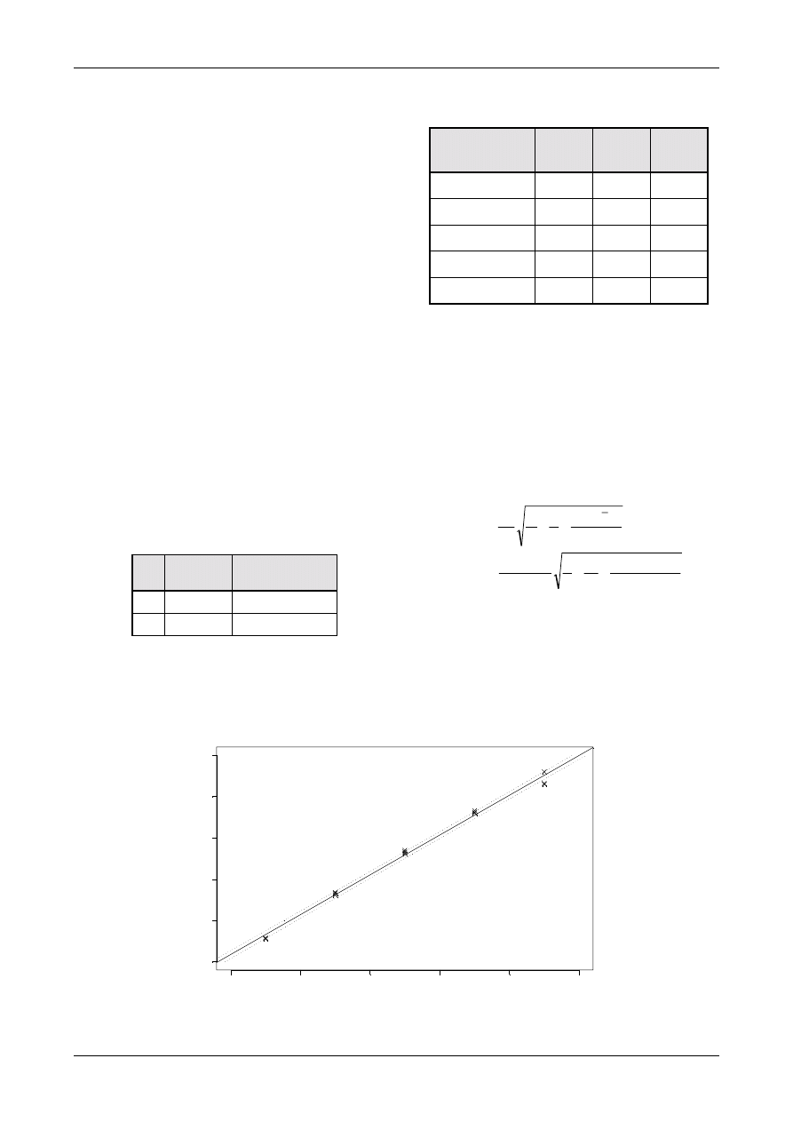
Quantifying Uncertainty

Example A5

QUAM:2000.1

Page 75

assumes that the uncertainties of the values of the
abscissa are considerably smaller than the
uncertainty on the values of the ordinate.
Therefore the usual uncertainty calculation
procedures for c

only reflect the uncertainty in

the absorbance and not the uncertainty of the
calibration standards, nor the inevitable
correlations induced by successive dilution from
the same stock. In this case, however, the
uncertainty of the calibration standards is
sufficiently small to be neglected.

The five calibration standards were measured
three times each, providing the results in Table
A5.2.

The calibration curve is given by

⋅

where

measurement of the absorbance of the i

calibration standard

:concentration of the i

calibration standard

:slope

:intercept

and the results of the linear least square fit are

Value

Standard

deviation

0.2410

0.0050

0.0087

0.0029

with a correlation coefficient r of 0.997. The

fitted line is shown in Figure A5.7. The residual
standard deviation S is 0.005486.

The actual leach solution was measured twice,
leading to a concentration c

of 0.26 mg l

-1

. The

calculation of the uncertainty u(c

) associated

with the linear least square fitting procedure is
described in detail in Appendix E3. Therefore
only a short description of the different
calculation steps is given here.

u(c

) is given by

018

)

(

)

(

241

005486

)

(

)

(

−

⇒

−

with the residual standard deviation S given by

Table A5.2: Calibration results

Concentration

[mg l

-1

]

0.1

0.028

0.029

0.3

0.084

0.083

0.081

0.5

0.135

0.131

0.133

0.7

0.180

0.181

0.183

0.9

0.215

0.230

0.216

Figure A5.7:Linear least square fit and uncertainty interval for duplicate determinations

Concentration of Cadmium [mg/l]

Absor

0.0

0.2

0.4

0.6

0.8

1.0

Quantifying Uncertainty

Example A5

QUAM:2000.1

Page 76

005486

)]

(

[

−

⋅

−

∑

and

)

(

−

∑

where

:slope

:number of measurements to determine c

:number of measurements for the
calibration

:determined cadmium concentration of
the leached solution

:mean value of the different calibration
standards (n number of measurements)

:index for the number of calibration
standards

:index for the number of measurements to
obtain the calibration curve

Area a

Length measurement

: The total surface area of the

sample vessel was calculated, from measured
dimensions, to be 2.37 dm

. Since the item is

approximately cylindrical but not perfectly
regular, measurements are estimated to be within
2 mm at 95% confidence. Typical dimensions are
between 1.0

dm and 2.0

dm leading to an

estimated dimensional measurement uncertainty
of 1 mm (after dividing the 95% figure by 1.96).
Area measurements typically require two length
measurements, height and width respectively (i.e.
1.45 dm and 1.64 dm)

Area

: Since the item has not a perfect geometric

shape, there is also an uncertainty in any area
calculation; in this example, this is estimated to
contribute an additional 5% at 95% confidence.

The uncertainty contribution of the length
measurement and area itself are combined in the
usual way.

)

(

)

(

⇒













Temperature effect f

temp

A number of studies of the effect of temperature
on metal release from ceramic ware have been
undertaken

(1-5)

. In general, the temperature effect

is substantial and a near-exponential increase in
metal release with temperature is observed until
limiting values are reached. Only one study

has

given an indication of effects in the range of 20-
25

C. From the graphical information presented

the change in metal release with temperature near
25

C is approximately linear, with a gradient of

approximately 5%

-1

. For the

C range

allowed by the empirical method this leads to a
factor f

temp

of 1

0.1. Converting this to a standard

uncertainty gives, assuming a rectangular
distribution:

temp

Time effect f

time

For a relatively slow process such as leaching, the
amount leached will be approximately
proportional to time for small changes in the time.
Krinitz and Franco

found a mean change in

concentration over the last six hours of leaching
of approximately 1.8 mg l

-1

in 86 mg l

-1

, that is,

about 0.3%/h. For a time of (24

0.5)h c

will

therefore need correction by a factor f

time

(0.5

0.003) =1

0.0015. This is a rectangular

distribution leading to the standard uncertainty

001

0015

)

(

≅

time

Acid concentration f

acid

One study of the effect of acid concentration on
lead release showed that changing concentration
from 4 to 5% v/v increased the lead released from
a particular ceramic batch from 92.9 to
101.9 mg l

-1

, i.e. a change in f

acid

097

)

101

(

−

or close to 0.1.

Another study, using a hot leach method, showed
a comparable change (50% change in lead
extracted on a change of from 2 to 6% v/v)

Assuming this effect as approximately linear with
acid concentration gives an estimated change in
f

acid

of approximately 0.1 per % v/v change in acid

concentration. In a separate experiment the
concentration and its standard uncertainty have
been established using titration with a
standardised NaOH titre (3.996%

= 0.008% v/v). Taking the uncertainty of

0.008% v/v on the acid concentration suggests an
uncertainty for f

acid

of 0.008

0.1 = 0.0008. As the

uncertainty on the acid concentration is already
expressed as a standard uncertainty, this value can
be used directly as the uncertainty associated with
f

acid

Quantifying Uncertainty

Example A5

QUAM:2000.1

Page 77

OTE

: In principle, the uncertainty value would need

correcting for the assumption that the single
study above is sufficiently representative of all
ceramics. The present value does, however,
give a reasonable estimate of the magnitude of
the uncertainty.

A5.5 Step 4: Calculating the combined

standard uncertainty

The amount of leached cadmium per unit area,
assuming no dilution, is given by

temp

time

acid

⋅

The intermediate values and their standard
uncertainties are collected in Table A5.3.
Employing those values

036

332

−

In order to calculate the combined standard
uncertainty of a multiplicative expression (as
above) the standard uncertainties of each
component are used as follows:

( )

(

)

(

)

( )

095

001

0008

025

0054

069











































































temp

time

acid

-2

0034

095

)

(

⇒

The simpler spreadsheet approach to calculate the
combined standard uncertainty is shown in Table

A5.4. A description of the method is given in
Appendix E.

The contributions of the different parameters and
influence quantities to the measurement
uncertainty are illustrated in Figure A5.8,
comparing the size of each of the contributions
(C13:H13 in Table A5.4) with the combined
uncertainty (B16).

The expanded uncertainty U(r) is obtained by
applying a coverage factor of 2

= 0.0034

2 = 0.007 mg dm

-2

Thus the amount of released cadmium measured
according to BS 6748:1986

(0.036

0.007) mg dm

-2

where the stated uncertainty is calculated using a
coverage factor of 2.

A5.6 References for Example 5

1. B. Krinitz, V. Franco, J. AOAC

56 869-875

(1973)

2. B. Krinitz, J. AOAC

61, 1124-1129 (1978)

3. J. H. Gould, S. W. Butler, K. W. Boyer, E. A.

Stelle, J. AOAC

66, 610-619 (1983)

4. T. D. Seht, S. Sircar, M. Z. Hasan, Bull.

Environ. Contam. Toxicol.

10, 51-56 (1973)

5. J. H. Gould, S. W. Butler, E. A. Steele, J.

AOAC

66, 1112-1116 (1983)

Table A5.3: Intermediate values and uncertainties for leachable cadmium analysis

Description

Value

Standard uncertainty

(x)

Relative standard

uncertainty u(x)/x

Content of cadmium in the extraction
solution

0.26 mg l

-1

0.018 mg l

-1

0.069

Volume of the leachate

0.332 l

0.0018 l

0.0054

Surface area of the vessel

2.37 dm

0.06 dm

0.025

acid

Influence of the acid concentration

1.0

0.0008

time

Influence of the duration

1.0

0.001

temp

Influence of temperature

1.0

0.06

Quantifying Uncertainty

Example A5

QUAM:2000.1

Page 78

Table A5.4: Spreadsheet calculation of uncertainty for leachable cadmium analysis

acid

time

temp

value

0.26

0.332

2.37

1.0

uncertainty 0.018

0.0018

0.06

0.0008

0.001

0.06

0.26

0.278

0.26

0.332

0.3338

0.332

2.37

2.43

2.37

acid

1.0

1.0008

1.0

time

1.0

1.001

1.0

temp

1.0

1.06

0.036422

0.038943

0.036619

0.035523

0.036451

0.036458

0.038607

u(y,x

)

0.002521

0.000197

-0.000899

0.000029

0.000036

0.002185

u(y)

u(y,x

)

1.199 E-5

6.36 E-6

3.90 E-8

8.09 E-7

8.49 E-10

1.33 E-9

4.78 E-6

(r)

0.0034

The values of the parameters are entered in the second row from C2 to H2, and their standard uncertainties in the row
below (C3:H3). The spreadsheet copies the values from C2:H2 into the second column (B5:B10). The result (r) using
these values is given in B12. C5 shows the value of c

from C2 plus its uncertainty given in C3. The result of the

calculation using the values C5:C10 is given in C12. The columns D and H follow a similar procedure. Row 13
(C13:H13) shows the differences of the row (C12:H12) minus the value given in B12. In row 14 (C14:H14) the values
of row 13 (C13:H13) are squared and summed to give the value shown in B14. B16 gives the combined standard
uncertainty, which is the square root of B14.

Figure A5.8: Uncertainties in leachable Cd determination

u(y,x

) (mg dm

-2

)x1000

c(0)

V(L)

a(V)

f(acid)

f(time)

f(temp)

The values of u(y,x

)=(

∂

).u(x

) are taken from Table A5.4

Quantifying Uncertainty

Example A6

QUAM:2000.1

Page 79

Example A6: The Determination of Crude Fibre in Animal Feeding Stuffs

Summary

Goal

The determination of crude fibre by a regulatory
standard method.

Measurement procedure

The measurement procedure is a standardised
procedure involving the general steps outlined in
Figure A6.1. These are repeated for a blank
sample to obtain a blank correction.

Measurand

The fibre content as a percentage of the sample by
weight, C

fibre

, is given by:

fibre

(

)

100

−

Where:

is the mass (g) of the sample.

(Approximately 1 g)

is the loss of mass (g) after ashing during

the determination;

is the loss of mass (g) after ashing during

the blank test.

Identification of uncertainty sources

A full cause and effect diagram is provided as
Figure A6.9.

Quantification of uncertainty components

Laboratory experiments showed that the method
was performing in house in a manner that fully
justified adoption of collaborative study

reproducibility data. No other contributions were
significant in general. At low levels it was
necessary to add an allowance for the specific
drying procedure used. Typical resulting
uncertainty estimates are tabulated below (as
standard uncertainties) (Table A6.1).

Figure A6.1: Fibre determination.

Alkaline digestion

Dry and

weigh residue

Dry and

weigh residue

Ash and weigh

residue

Ash and weigh

residue

RESULT

Acid digestion

Grind and

weigh sample

Grind and

weigh sample

Table A6.1: Combined standard uncertainties

Fibre content

(%w/w)

Standard uncertainty

fibre

) (%w/w)

Relative Standard uncertainty

fibre

) / C

fibre

2.5

0 29

0 115

0 31

0.12

0.4

0.08

0.6

0.06

Quantifying Uncertainty

Example A6

QUAM:2000.1

Page 80

Example A6:The determination of crude fibre in animal feeding stuffs.

Detailed discussion

A6.1 Introduction

Crude fibre is defined in the method scope as the
amount of fat-free organic substances which are
insoluble in acid and alkaline media. The
procedure is standardised and its results used
directly. Changes in the procedure change the
measurand; this is accordingly an example of an
empirical method.

Collaborative trial data (repeatability and
reproducibility) were available for this statutory
method. The precision experiments described
were planned as part of the in-house evaluation of
the method performance. There is no suitable
reference material (i.e. certified by the same
method) available for this method.

A6.2 Step 1: Specification

Procedure

The procedure, a complex digestion, filtration,
drying, ashing and weighing procedure, which is
also repeated for a blank crucible, is summarised
in Figure A6.2. The aim is to digest most
components, leaving behind all the undigested
material. The organic material is ashed, leaving
an inorganic residue. The difference between the
dry organic/inorganic residue weight and the
ashed residue weight is the “fibre content”. The
main stages are:

Grind the sample to pass through a 1mm
sieve

ii) Weigh 1g of the sample into a weighed

crucible

iii) Add a set of acid digestion reagents at stated

concentrations and volumes. Boil for a
stated, standardised time, filter and wash the
residue.

iv) Add standard alkali digestion reagents and

boil for the required time, filter, wash and
rinse with acetone.

v) Dry to constant weight at a standardised

temperature (“constant weight” is not
defined within the published method; nor are
other drying conditions such as air
circulation or dispersion of the residue).

vi) Record the dry residue weight.

vii) Ash at a stated temperature to “constant

weight” (in practice realised by ashing for a
set time decided after in house studies).

viii) Weigh the ashed residue and calculate the

fibre content by difference, after subtracting
the residue weight found for the blank
crucible.

Measurand

The fibre content as a percentage of the sample by
weight, C

fibre

, is given by:

fibre

(

)

100

−

Where:

is the mass (g) of the sample. Approximately
1 g of sample is taken for analysis.

is the loss of mass (g) after ashing during the
determination.

is the loss of mass (g) after ashing during the
blank test.

A6.3 Step 2: Identifying and analysing

uncertainty sources

A range of sources of uncertainty was identified.
These are shown in the cause and effect diagram
for the method (see Figure A6.9). This diagram
was simplified to remove duplication following
the procedures in Appendix D; this, together with
removal of insignificant components, leads to the
simplified cause and effect diagram in Figure
A6.10.

Since prior collaborative and in-house study data
were available for the method, the use of these
data is closely related to the evaluation of
different contributions to uncertainty and is
accordingly discussed further below.

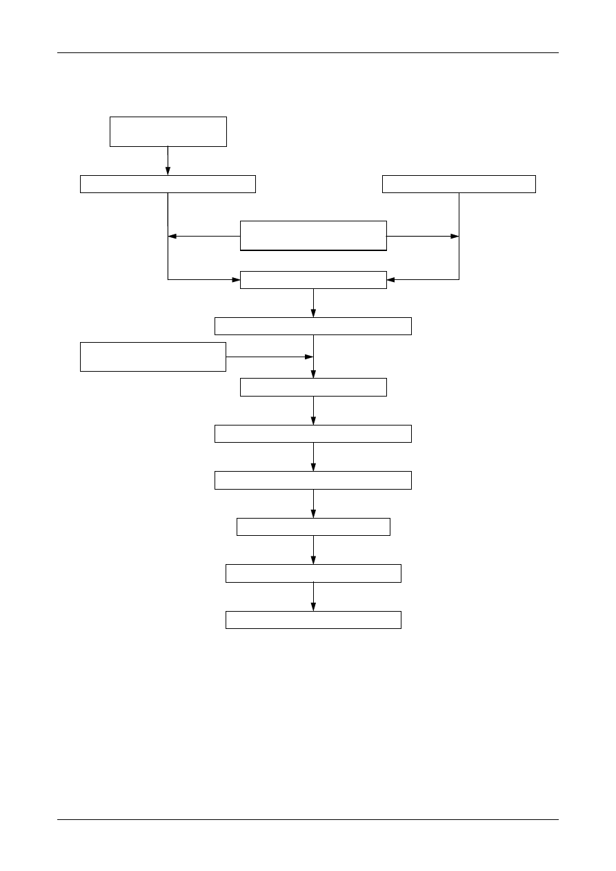
Quantifying Uncertainty

Example A6

QUAM:2000.1

Page 81

A6.4 Step 3: Quantifying uncertainty

components

Collaborative trial results

The method has been the subject of a
collaborative trial. Five different feeding stuffs
representing typical fibre and fat concentrations
were analysed in the trial. Participants in the trial
carried out all stages of the method, including
grinding of the samples. The repeatability and

reproducibility estimates obtained from the trial
are presented in Table A6.2.

As part of the in-house evaluation of the method,
experiments were planned to evaluate the
repeatability (within batch precision) for feeding
stuffs with fibre concentrations similar to those of
the samples analysed in the collaborative trial.
The results are summarised in Table A6.2. Each
estimate of in-house repeatability is based on 5
replicates.

Figure A6.2: Flow diagram illustrating the stages in the regulatory method for the

determination of fibre in animal feeding stuffs

Grind sample to pass

through 1 mm sieve

Weigh 1 g of sample into crucible

Add filter aid, anti-foaming agent

followed by 150 ml boiling H

Add anti-foaming agent followed

by 150 ml boiling KOH

Boil vigorously for 30 mins

Filter and wash with 3x30 ml boiling water

Boil vigorously for 30 mins

Filter and wash with 3x30 ml boiling water

Apply vacuum, wash with 3x25 ml acetone

Dry to constant weight at 130 °C

Ash to constant weight at 475-500 °C

Calculate the % crude fibre content

Weigh crucible for blank test

Quantifying Uncertainty

Example A6

QUAM:2000.1

Page 82

The estimates of repeatability obtained in-house
were comparable to those obtained from the
collaborative trial. This indicates that the method
precision in this particular laboratory is similar to
that of the laboratories which took part in the
collaborative trial. It is therefore acceptable to
use the reproducibility standard deviation from
the collaborative trial in the uncertainty budget
for the method. To complete the uncertainty
budget we need to consider whether there are any
other effects not covered by the collaborative trial
which need to be addressed. The collaborative
trial covered different sample matrices and the
pre-treatment of samples, as the participants were
supplied with samples which required grinding
prior to analysis. The uncertainties associated
with matrix effects and sample pre-treatment do
not therefore require any additional consideration.
Other parameters which affect the result relate to
the extraction and drying conditions used in the
method. These were investigated separately to
ensure the laboratory bias was under control (i.e.,
small compared to the reproducibility standard
deviation). The parameters considered are
discussed below.

Loss of mass on ashing

As there is no appropriate reference material for
this method, in-house bias has to be assessed by
considering the uncertainties associated with
individual stages of the method. Several factors
will contribute to the uncertainty associated with
the loss of mass after ashing:
! acid concentration;

! alkali concentration;
! acid digestion time;
! alkali digestion time;
! drying temperature and time;
! ashing temperature and time.

Reagent concentrations and digestion times

The effects of acid concentration, alkali
concentration, acid digestion time and alkali
digestion time have been studied in previously
published papers. In these studies, the effect of
changes in the parameter on the result of the
analysis was evaluated. For each parameter the
sensitivity coefficient (i.e., the rate of change in
the final result with changes in the parameter) and
the uncertainty in the parameter were calculated.

The uncertainties given in Table A6.3 are small
compared to the reproducibility figures presented
in Table A6.2. For example, the reproducibility
standard deviation for a sample containing
2.3 % w/w fibre is 0.293 % w/w. The uncertainty
associated with variations in the acid digestion
time is estimated as 0.021

w/w (i.e.,

2.3

0.009). We can therefore safely neglect the

uncertainties associated with variations in these
method parameters.

Drying temperature and time

No prior data were available. The method states
that the sample should be dried at 130 °C to
“constant weight”. In this case the sample is dried
for 3 hours at 130 °C and then weighed. It is then
dried for a further hour and re-weighed. Constant

Table A6.2: Summary of results from collaborative trial of the method and in-house

repeatability check

Fibre content (% w/w)

Collaborative trial results

Sample

Mean

Reproducibility

standard

deviation (s

)

Repeatability

standard

deviation (s

)

In-house

repeatability

standard

deviation

0.293

0.198

0.193

12.1

0.563

0.358

0.312

5.4

0.390

0.264

0.259

3.4

0.347

0.232

0.213

10.1

0.575

0.391

0.327

Quantifying Uncertainty

Example A6

QUAM:2000.1

Page 83

weight is defined in this laboratory as a change of
less than 2 mg between successive weighings. In
an in-house study, replicate samples of four
feeding stuffs were dried at 110, 130 and 150 °C
and weighed after 3 and 4 hours drying time. In
the majority of cases, the weight change between
3 and 4 hours was less than 2 mg. This was
therefore taken as the worst case estimate of the
uncertainty in the weight change on drying. The
range ±2 mg describes a rectangular distribution,
which is converted to a standard uncertainty by
dividing by

√

3. The uncertainty in the weight

recorded after drying to constant weight is
therefore 0.00115

g. The method specifies a

sample weight of 1 g. For a 1 g sample, the
uncertainty in drying to constant weight
corresponds to a standard uncertainty of
0.115 % w/w in the fibre content. This source of
uncertainty is independent of the fibre content of
the sample. There will therefore be a fixed
contribution of 0.115 % w/w to the uncertainty
budget for each sample, regardless of the
concentration of fibre in the sample. At all fibre
concentrations, this uncertainty is smaller than the
reproducibility standard deviation, and for all but
the lowest fibre concentrations is less than 1/3 of
the s

value. Again, this source of uncertainty can

usually be neglected. However for low fibre
concentrations, this uncertainty is more than 1/3
of the s

value so an additional term should be

included in the uncertainty budget (see Table
A6.4).

Ashing temperature and time

The method requires the sample to be ashed at
475 to 500 °C for at least 30 mins. A published
study on the effect of ashing conditions involved
determining fibre content at a number of different
ashing temperature/time combinations, ranging
from 450 °C for 30 minutes to 650 °C for 3 hours.
No significant difference was observed between
the fibre contents obtained under the different
conditions. The effect on the final result of small
variations in ashing temperature and time can
therefore be assumed to be negligible.

Loss of mass after blank ashing

No experimental data were available for this
parameter. However, as discussed above, the
effects of variations in this parameter are likely to
be small.

A6.5 Step 4: Calculating the combined

standard uncertainty

This is an example of an empirical method for
which collaborative trial data were available. The
in-house repeatability was evaluated and found to
be comparable to that predicted by the
collaborative trial. It is therefore appropriate to
use the s

values from the collaborative trial. The

discussion presented in Step

3 leads to the

Table A6.3: Uncertainties associated with method parameters

Parameter

Sensitivity

coefficient

Note 1

Uncertainty in

parameter

Uncertainty in final

result as RSD

Note 4

acid concentration

0.23 (mol l

-1

)

-1

0.0013 mol l

-1

Note 2

0.00030

alkali concentration

0.21 (mol l

-1

)

-1

0.0023 mol l

-1

Note 2

0.00048

acid digestion time

0.0031 min

-1

2.89 mins

Note 3

0.0090

alkali digestion time

0.0025 min

-1

2.89 mins

Note 3

0.0072

Note 1.The sensitivity coefficients were estimated by plotting the normalised change in fibre content against

reagent strength or digestion time. Linear regression was then used to calculate the rate of change of the
result of the analysis with changes in the parameter.

Note 2.The standard uncertainties in the concentrations of the acid and alkali solutions were calculated from

estimates of the precision and trueness of the volumetric glassware used in their preparation, temperature
effects etc. See examples A1-A3 for further examples of calculating uncertainties for the concentrations of
solutions.

Note 3.The method specifies a digestion time of 30 minutes. The digestion time is controlled to within ±5

minutes. This is a rectangular distribution which is converted to a standard uncertainty by dividing by

√

Note 4.The uncertainty in the final result, as a relative standard deviation, is calculated by multiplying the

sensitivity coefficient by the uncertainty in the parameter.

Quantifying Uncertainty

Example A6

QUAM:2000.1

Page 84

conclusion that, with the exception of the effect
of drying conditions at low fibre concentrations,
the other sources of uncertainty identified are all
small in comparison to s

. In cases such as this,

the uncertainty estimate can be based on the
reproducibility standard deviation, s

, obtained

from the collaborative trial. For samples with a
fibre content of 2.5 % w/w, an additional term has
been included to take account of the uncertainty
associated with the drying conditions.

Standard uncertainty

Typical standard uncertainties for a range of fibre
concentrations are given in the Table A6.4 below.

Expanded uncertainty

Typical expanded uncertainties are given in Table
A6.5 below. These were calculated using a
coverage factor k of 2, which gives a level of
confidence of approximately 95%.

Table A6.4: Combined standard uncertainties

Fibre content

(% w/w)

Standard uncertainty

fibre

) (%w/w)

Relative standard uncertainty

fibre

) / C

fibre

2.5

0 29

0 115

0 31

0.12

0.4

0.08

0.6

0.06

Table A6.5: Expanded uncertainties

Fibre content

(% w/w)

Expanded uncertainty

U(C

fibre

) (% w/w)

Expanded uncertainty

(% of fibre content)

2.5

0.62

0.8

0.12

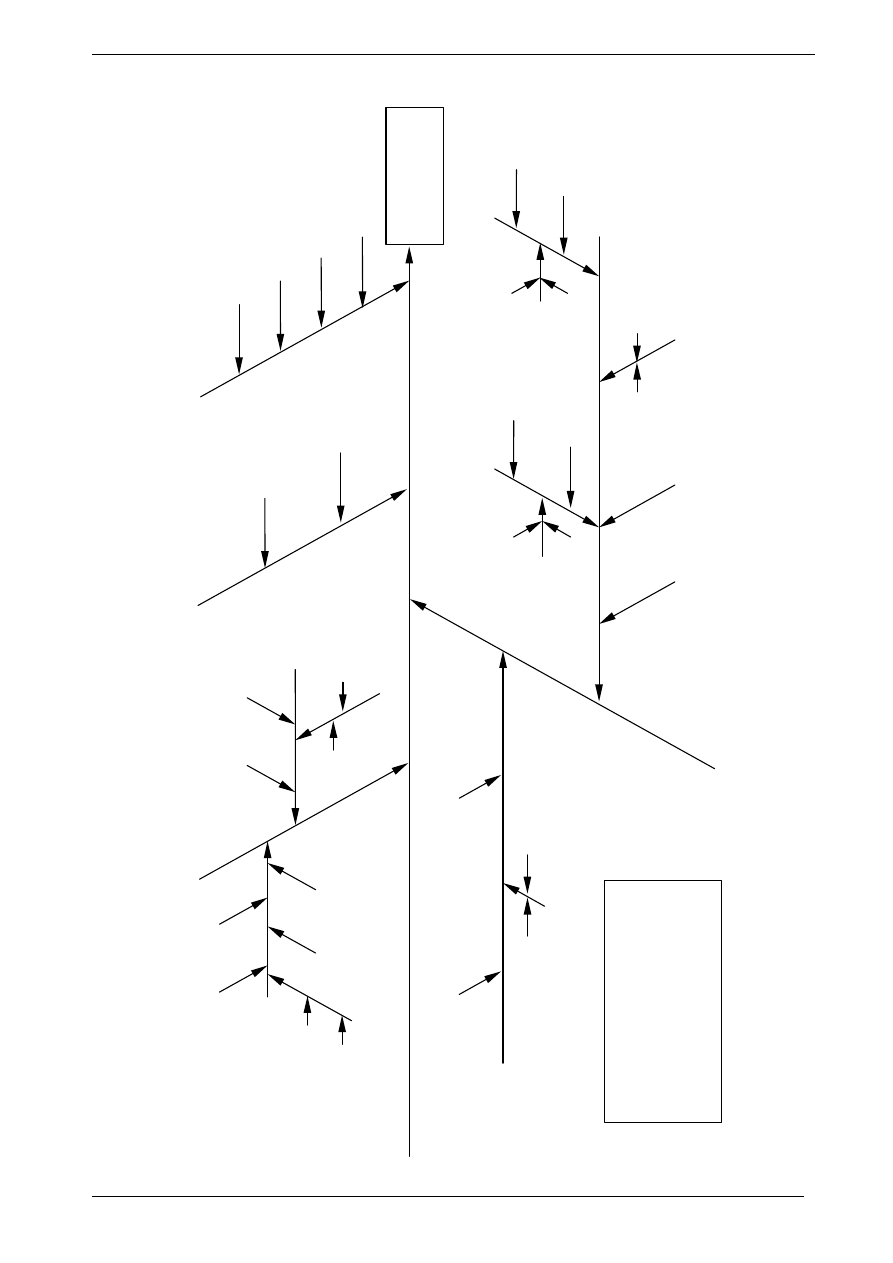
Figure A6.9: Cause and effect diagram for the determination of fibre in animal feeding stuffs

Crude Fibre

(%)

Loss of mass after ashing (b)

Loss of mass after blank ashing (c)

Mass sample (a)

Precision

sample weight precision

weighing precision

weight of crucible

before ashing

drying temp

weight of sample

and crucible

after ashing

ashing temp

ashing time

weighing of crucible

balance linearity

balance calibration

extraction precision

weight of

crucible after

ashing

drying time

balance calibration

balance linearity

ashing temp

ashing time

balance

calibration

balance

linearity

weighing of crucible

acid digest

alkali digest

alkali

volume

alkali conc

digest conditions

boiling rate

extraction time

acid vol

acid conc

digest conditions

boiling rate

extraction time

balance linearity

balance calibration

drying temp

drying time

weighing of crucible

ashing precision

balance calibration

balance linearity

weight of sample

and crucible before

ashing

acid digest*

alkali digest*

*The branches feeding into these “acid

digest” and “alkali digest” branches

have been omitted for clarity. The

same factors affect them as for the

sample (i.e., digest conditions, acid

conc

etc.

QUAM:2000.1

Page 85

Quantifying Uncertainty

Example A6

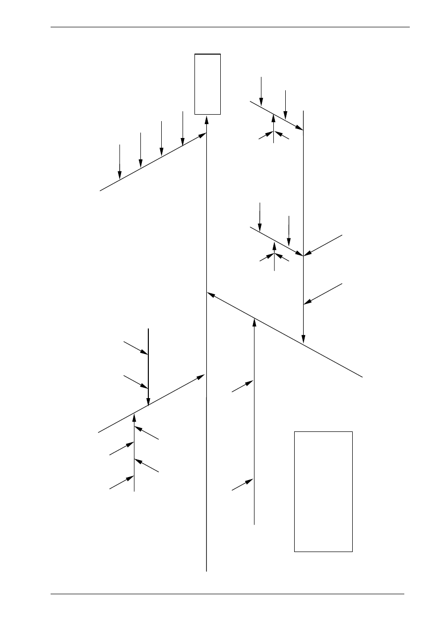
Figure A6.10: Simplified cause and effect diagram

alkali vol

Crude Fibre

(%)

Loss of mass after ashing (b)

Loss of mass after blank ashing (c)

Precision

sample weight precision

weighing precision

weight of crucible

before ashing

drying temp

ashing temp

ashing time

extraction

weight of

crucible after

ashing

drying time

ashing temp

ashing time

acid digest

alkali digest

alkali conc

digest conditions

boiling rate

extraction time

acid vol

acid conc

digest conditions

boiling rate

extraction time

drying temp

drying time

ashing precision

weight of sample and

crucible after ashing

weight of sample

and crucible before

ashing

acid digest*

alkali digest*

*The branches feeding into these “acid

digest” and “alkali digest” branches

have been omitted for clarity. The

same factors affect them as for the

sample (i.e., digest conditions, acid

conc

etc.

QUAM:2000.1

Page 86

Quantifying Uncertainty

Example A6

Quantifying Uncertainty

Example A7

QUAM:2000.1

Page 87

Example A7: Determination of the Amount of Lead in Water Using Double

Isotope Dilution and Inductively Coupled Plasma Mass Spectrometry

A7.1 Introduction

This example illustrates how the uncertainty
concept can be applied to a measurement of the
amount content of lead in a water sample using
Isotope Dilution Mass Spectrometry (IDMS) and
Inductively Coupled Plasma Mass Spectrometry
(ICP-MS).

General introduction to Double IDMS

IDMS is one of the techniques that is recognised
by the Comité consultatif pour la quantité de
matière (CCQM) to have the potential to be a
primary method of measurement, and therefore a
well defined expression which describes how the
measurand is calculated is available. In the
simplest case of isotope dilution using a certified
spike, which is an enriched isotopic reference
material, isotope ratios in the spike, the sample
and a blend b of known masses of sample and
spike are measured. The element amount content
c

in the sample is given by:

(

)

(

)

∑

⋅

−

⋅

−

⋅

(1)

where c

and c

are element amount content in the

sample and the spike respectively (the symbol c is
used here instead of k for amount content

avoid confusion with K-factors and coverage
factors k). m

and m

are mass of sample and spike

respectively. R

, R

and R

are the isotope amount

ratios. The indexes x, y and b represent the
sample, the spike and the blend respectively. One
isotope, usually the most abundant in the sample,
is selected and all isotope amount ratios are
expressed relative to it. A particular pair of
isotopes, the reference isotope and preferably the
most abundant isotope in the spike, is then
selected as monitor ratio, e.g. n(

208

Pb)/n(

206

Pb).

and R

are all the possible isotope amount

ratios in the sample and the spike respectively.
For the reference isotope, this ratio is unity. K

and K

are the correction factors for mass

discrimination, for a particular isotope amount
ratio, in sample, spike and blend respectively. The
K

-factors are measured using a certified isotopic

reference material according to equation (2).

observed

certified

bias

where

;

(2)

where K

is the mass discrimination correction

factor at time 0, K

bias

is a bias factor coming into

effect as soon as the K-factor is applied to correct
a ratio measured at a different time during the
measurement. The K

bias

also includes other

possible sources of bias such as multiplier dead
time correction, matrix effects etc. R

certified

is the

certified isotope amount ratio taken from the
certificate of an isotopic reference material and
R

observed

is the observed value of this isotopic

reference material. In IDMS experiments, using
Inductively Coupled Plasma Mass Spectrometry
(ICP-MS), mass fractionation will vary with time
which requires that all isotope amount ratios in
equation (1) need to be individually corrected for
mass discrimination.

Certified material enriched in a specific isotope is
often unavailable. To overcome this problem,
‘double’ IDMS is frequently used. The procedure
uses a less well characterised, isotopically
enriched spiking material in conjunction with a
certified material (denoted z) of natural isotopic
composition. The certified, natural composition
material acts as the primary assay standard. Two
blends are used; blend b is a blend between
sample and enriched spike, as in equation (1). To
perform double IDMS a second blend, b’ is
prepared from the primary assay standard with
amount content c

, and the enriched material y.

This gives a similar expression to equation (1):

(

)

(

)

∑

⋅

−

⋅

−

⋅

(3)

where c

is the element amount content of the

primary assay standard solution and m

the mass

of the primary assay standard when preparing the
new blend. m’

is the mass of the enriched spike

solution, K’

, R’

, K

and R

are the K-factor and

the ratio for the new blend and the assay standard
respectively. The index z represents the assay

Quantifying Uncertainty

Example A7

QUAM:2000.1

Page 88

standard. Dividing equation (1) with equation (3)
gives

(

)

(

)

(

)

(

)

∑

⋅

−

⋅

−

⋅

−

⋅

−

⋅

(4)

Simplifying this equation and introducing a
procedure blank, c

blank

, we get:

(

)

(

)

blank

−

⋅

−

⋅

−

⋅

−

⋅

−

⋅

∑

(5)

This is the final equation, from which c

has been

eliminated. In this measurement the number index
on the amount ratios, R, represents the following
actual isotope amount ratios:

=n(

208

Pb)/n(

206

Pb)

=n(

206

Pb)/n(

206

Pb)

=n(

207

Pb)/n(

206

Pb)

=n(

204

Pb)/n(

206

Pb)

For reference, the parameters are summarised in
Table A7.1.

A7.2 Step 1: Specification

The general procedure for the measurements is
shown in Table A7.2. The calculations and
measurements involved are described below.

Calculation procedure for the amount content c

For this determination of lead in water, four
blends each of b’, (assay + spike), and b, (sample
+ spike), were prepared. This gives a total of 4
values for c

. One of these determinations will be

described in detail following Table A7.2, steps 1
to 4. The reported value for c

will be the average

of the four replicates.

Table A7.1. Summary of IDMS parameters

Parameter

Description

Parameter

Description

mass of sample in blend b [g]

mass of enriched spike in blend b [g]

mass of enriched spike in blend b’
[g]

mass of primary assay standard in
blend b’ [g]

amount content of the sample x
[mol g

-1

mol g

-1

]

Note 1

amount content of the primary assay
standard z [mol g

-1

mol g

-1

]

Note 1

amount content of the spike y
[mol g

-1

mol g

-1

]

Note 1

blank

observed amount content in procedure
blank [mol g

-1

mol g

-1

]

Note 1

measured ratio of blend b,
n(

208

Pb)/n(

206

Pb)

mass bias correction of R

measured ratio of blend b’,
n(

208

Pb)/n(

206

Pb)

mass bias correction of R’

measured ratio of enriched isotope
to reference isotope in the enriched
spike

mass bias correction of R

all ratios in the primary assay
standard, R

, R

etc.

mass bias correction factors for R

all ratios in the sample

mass bias correction factors for R

measured ratio of enriched isotope
to reference isotope in the sample x

as R

but in the primary assay

standard

Note 1: Units for amount content are always specified in the text.

Quantifying Uncertainty

Example A7

QUAM:2000.1

Page 89

Table A7.2. General procedure

Step

Description

Preparing the primary assay
standard

Preparation of blends: b’ and b

Measurement of isotope ratios

Calculation of the amount
content of Pb in the sample, c

Estimating the uncertainty in c

Calculation of the Molar Mass

Due to natural variations in the isotopic
composition of certain elements, e.g. Pb, the
molar mass, M, for the primary assay standard has
to be determined since this will affect the amount
content c

. Note that this is not the case when c

expressed in mol g

-1

. The molar mass, M(E), for

an element E, is numerically equal to the atomic
weight of element E, A

(E). The atomic weight

can be calculated according to the general
expression:

( )

∑

⋅

)

(

(6)

where the values R

are all true isotope amount

ratios for the element E and M(

E) are the

tabulated nuclide masses.

Note that the isotope amount ratios in equation
(6) have to be absolute ratios, that is, they have to
be corrected for mass discrimination. With the
use of proper indexes, this gives equation (7). For
the calculation, nuclide masses, M(

E), were taken

from literature values

, while Ratios, R

, and K

factors, K

(zi), were measured (see Table A7.8).

These values give

( )

mol

21034

207

)

Assay

(

−

⋅

∑

(7)

Measurement of K-factors and isotope amount
ratios

To correct for mass discrimination, a correction
factor, K, is used as specified in equation (2). The
K

-factor can be calculated using a reference

material certified for isotopic composition. In this
case, the isotopically certified reference material
NIST SRM 981 was used to monitor a possible
change in the K

-factor. The K

-factor is measured

before and after the ratio it will correct. A typical
sample sequence is: 1. (blank), 2. (NIST SRM
981), 3. (blank), 4. (blend 1), 5. (blank), 6. (NIST
SRM 981), 7. (blank), 8. (sample), etc.

The blank measurements are not only used for
blank correction, they are also used for
monitoring the number of counts for the blank.
No new measurement run was started until the
blank count rate was stable and back to a normal
level. Note that sample, blends, spike and assay
standard were diluted to an appropriate amount
content prior to the measurements. The results of
ratio measurements, calculated K

-factors and K

bias

are summarised in Table A7.8.

Preparing the primary assay standard and
calculating the amount content, c

Two primary assay standards were produced,
each from a different piece of metallic lead with a
chemical purity of w=99.999 %. The two pieces
came from the same batch of high purity lead.
The pieces were dissolved in about 10 ml of 1:3
w/w HNO

:water under gentle heating and then

further diluted. Two blends were prepared from
each of these two assay standards. The values
from one of the assays is described hereafter.

0.36544 g lead, m

, was dissolved and diluted in

aqueous HNO

(0.5 mol l

-1

) to a total of

=196.14 g. This solution is named Assay 1. A

more diluted solution was needed and m

=1.0292

g of Assay 1, was diluted in aqueous HNO

(0.5 mol l

-1

) to a total mass of d

=99.931g. This

solution is named Assay 2. The amount content of
Pb in Assay 2, c

, is then calculated according to

equation (8)

(

)

mol

092605

mol

2605

−

⋅

Assay

(8)

Preparation of the blends

The mass fraction of the spike is known to be
roughly 20µg Pb per g solution and the mass
fraction of Pb in the sample is also known to be in
this range. Table A7.3 shows the weighing data
for the two blends used in this example.

Quantifying Uncertainty

Example A7

QUAM:2000.1

Page 90

Measurement of the procedure blank c

Blank

In this case, the procedure blank was measured
using external calibration. A more exhaustive
procedure would be to add an enriched spike to a
blank and process it in the same way as the
samples. In this example, only high purity
reagents were used, which would lead to extreme
ratios in the blends and consequent poor
reliability for the enriched spiking procedure. The
externally calibrated procedure blank was
measured four times, and c

Blank

found to be

4.5

-7

µmol g

-1

, with standard uncertainty

4.0

-7

µmol g

-1

evaluated as type A.

Calculation of the unknown amount content c

Inserting the measured and calculated data (Table
A7.8) into equation (5) gives c

=0.053738

µmol g

-1

. The results from all four replicates are

given in Table A7.4.

A7.3 Steps 2 and 3: Identifying and

quantifying uncertainty sources

Strategy for the uncertainty calculation

If equations (2), (7) and (8) were to be included in
the final IDMS equation (5), the sheer number of
parameters would make the equation almost
impossible to handle. To keep it simpler, K

factors and amount content of the standard assay
solution and their associated uncertainties are
treated separately and then introduced into the
IDMS equation (5). In this case it will not affect
the final combined uncertainty of c

, and it is

advisable to simplify for practical reasons.

For calculating the combined standard
uncertainty, u

), the values from one of the

measurements, as described in A7.2, will be used.
The combined uncertainty of c

will be calculated

using the spreadsheet method described in
Appendix E.

Uncertainty on the K-factors

i) Uncertainty on K

K is calculated according to equation (2) and
using the values of K

as an example gives for

9992

1699

1681

)

(

observed

certified

(9)

To calculate the uncertainty on K

we first look at

the certificate where the certified ratio, 2.1681,
has a stated uncertainty of 0.0008 based on a 95%
confidence interval. To convert an uncertainty
based on a 95% confidence interval to standard
uncertainty we divide by 2. This gives a standard
uncertainty of u(R

certified

)=0.0004. The observed

amount ratio, R

observed

=n(

208

Pb)/n(

206

Pb), has a

standard uncertainty of 0.0025 (as rsd). For the K-
factor, the combined uncertainty can be calculated
as:

(

)

002507

0025

1681

0004

)

(

))

(













(10)

This clearly points out that the uncertainty
contributions from the certified ratios are
negligible. Henceforth, the uncertainties on the
measured ratios, R

observed

, will be used for the

uncertainties on K

Uncertainty on K

bias

This bias factor is introduced to account for
possible deviations in the value of the mass
discrimination factor. As can be seen in the cause
and effect diagram above, and in equation (2),
there is a bias associated with every K-factor. The
values of these biases are in our case not known,
and a value of 0 is applied. An uncertainty is, of

Table A7.3

Blend

b’

Solutions
used

Spike

Sample

Spike

Assay 2

Parameter

m’

Mass (g)

1.1360

1.0440

1.0654

1.1029

Table A7.4

(µmol g

-1

)

Replicate 1 (our example)

0.053738

Replicate 2

0.053621

Replicate 3

0.053610

Replicate 4

0.053822

Average

0.05370

Experimental standard
deviation (s)

0.0001

Quantifying Uncertainty

Example A7

QUAM:2000.1

Page 91

course, associated with every bias and this has to
be taken into consideration when calculating the
final uncertainty. In principle, a bias would be
applied as in equation (11), using an excerpt from
equation (5) and the parameters K

and R

demonstrate this principle.

(

)

(

)

(

bias

⋅

−

⋅

(11)

The values of all biases, K

bias

(yi, xi, zi), are (0

0.001). This estimation is based on a long
experience of lead IDMS measurements. All
K

bias

(yi, xi, zi) parameters are not included in

detail in Table A7.5, Table A7.8 or in equation 5,
but they are used in all uncertainty calculations.

Uncertainty of the weighed masses

In this case, a dedicated mass metrology lab
performed the weighings. The procedure applied
was a bracketing technique using calibrated
weights and a comparator. The bracketing
technique was repeated at least six times for every
sample mass determination. Buoyancy correction
was applied. Stoichiometry and impurity
corrections were not applied in this case. The
uncertainties from the weighing certificates were
treated as standard uncertainties and are given in

Table A7.8.

Uncertainty in the amount content of the Standard
Assay Solution, c

i) Uncertainty in the atomic weight of Pb

First, the combined uncertainty of the molar mass
of the assay solution, Assay 1, will be calculated.
The values in Table A7.5 are known or have been
measured:

According to equation (7), the calculation of the
molar mass takes this form:

)

(

Assay

⋅

(12)

To calculate the combined standard uncertainty of
the molar mass of Pb in the standard assay
solution, the spreadsheet model described in
Appendix E was used. There were eight
measurements of every ratio and K

. This gave a

molar mass M(Pb, Assay 1)=207.2103 g mol

-1

with uncertainty 0.0010 g mol

-1

calculated using

the spreadsheet method.

ii) Calculation of the combined standard
uncertainty in determining c

To calculate the uncertainty on the amount
content of Pb in the standard assay solution, c

the

data from A7.2 and equation (8) are used. The
uncertainties were taken from the weighing
certificates, see A7.3. All parameters used in
equation (8) are given with their uncertainties in
Table A7.6.

The amount content, c

, was calculated using

equation (8). Following Appendix D.5 the
combined standard uncertainty in c

, is calculated

to be u

)=0.000028. This gives

=0.092606 µmol g

-1

with a standard uncertainty

of 0.000028 µmol g

-1

(0.03% as %rsd).

To calculate u

), for replicate 1, the spreadsheet

model was applied (Appendix E). The uncertainty
budget for replicate 1 will be representative for
the measurement. Due to the number of
parameters in equation (5), the spreadsheet will
not be displayed. The value of the parameters and
their uncertainties as well as the combined
uncertainty of c

can be seen in Table A7.8.

Table A7.5

Value

Standard

Uncertainty

Type

Note 1

bias

(zi)

0.001

2.1429

0.0054

(z1)

0.9989

0.0025

(z3)

0.9993

0.0035

(z4)

1.0002

0.0060

0.9147

0.0032

0.05870

0.00035

207.976636

0.000003

205.974449

0.000003

206.975880

0.000003

203.973028

0.000003

Note 1. Type A (statistical evaluation) or Type B (other)

Quantifying Uncertainty

Example A7

QUAM:2000.1

Page 92

A7.4 Step 4: Calculating the combined

standard uncertainty

The average and the experimental standard
deviation of the four replicates are displayed in
Table A7.7. The numbers are taken from Table
A7.4 and Table A7.8.

Table A7.7

Replicate 1

Mean of replicates

1-4

= 0.05374

= 0.05370

µmol g

-1

)= 0.00018

0.00010

Note 1

µmol g

-1

Note 1.This is the experimental standard uncertainty and not
the standard deviation of the mean.

In IDMS, and in many non-routine analyses, a
complete statistical control of the measurement
procedure would require limitless resources and

time. A good way then to check if some source of
uncertainty has been forgotten is to compare the
uncertainties from the type A evaluations with the
experimental standard deviation of the four
replicates. If the experimental standard deviation
is higher than the contributions from the
uncertainty sources evaluated as type A, it could
indicate that the measurement process is not fully
understood. As an approximation, using data from
Table 8, the sum of the type A evaluated
experimental uncertainties can be calculated by
taking 92.2% of the total experimental
uncertainty, which is 0.00041 µmol

-1

. This

value is then clearly higher than the experimental
standard deviation of 0.00010 µmol g

-1

, see Table

A7.7. This indicates that the experimental
standard deviation is covered by the contributions
from the type A evaluated uncertainties and that
no further type A evaluated uncertainty
contribution, due to the preparation of the blends,
needs to be considered. There could however be a
bias associated with the preparations of the
blends. In this example, a possible bias in the
preparation of the blends is judged to be
insignificant in comparison to the major sources
of uncertainty.

The amount content of lead in the water sample is
then:

=(0.05370±0.00036) µmol g

-1

The result is presented with an expanded
uncertainty using a coverage factor of 2.

References for Example 7

1. T. Cvitaš, Metrologia, 1996,

33, 35-39

2 G. Audi and A.H. Wapstra, Nuclear Physics,

A565 (1993)

Table A7.6

Value

Uncertainty

Mass of lead piece, m

(g)

0.36544

0.00005

Total mass first dilution,
d

(g)

196.14

0.03

Aliquot of first dilution,
m

(g)

1.0292

0.0002

Total mass of second
dilution, d

(g)

99.931

0.01

Purity of the metallic
lead piece, w (mass
fraction)

0.99999

0.000005

Molar mass of Pb in the
Assay Material, M
(g mol

-1

)

207.2104

0.0010

Quantifying Uncertainty

Example A7

QUAM:2000.1

Page 93

Table A7.8

parameter uncertainty

evaluation

value

experimental

uncertainty

(Note 1)

contribution

to total u

(%)

final

uncertainty

(Note 2)

contribution

to total

(%)

bias

0.001

Note 3

7.2

0.001

Note 3

37.6

0.092605

0.000028

0.2

0.000028

0.8

(b)

0.9987

0.0025

14.4

0.00088

9.5

(b’)

0.9983

0.0025

18.3

0.00088

11.9

(x1)

0.9992

0.0025

4.3

0.00088

2.8

(x3)

1.0004

0.0035

0.0012

0.6

(x4)

1.001

0.006

0.0021

(y1)

0.9999

0.0025

0.00088

(z1)

0.9989

0.0025

6.6

0.00088

4.3

(z3)

0.9993

0.0035

0.0012

0.6

(z4)

1.0002

0.006

0.0021

1.0440

0.0002

0.1

0.0002

0.3

1.1360

0.0002

0.1

0.0002

0.3

1.0654

0.0002

0.1

0.0002

0.3

1.1029

0.0002

0.1

0.0002

0.3

0.29360

0.00073

14.2

0.00026

Note 4

9.5

R’

0.5050

0.0013

19.3

0.00046

12.7

2.1402

0.0054

4.4

0.0019

2.9

Cons.

0.9142

0.0032

0.0011

0.6

0.05901

0.00035

0.00012

0.00064

0.00004

0.000014

2.1429

0.0054

6.7

0.0019

4.4

Cons.

0.9147

0.0032

0.0011

0.6

0.05870

0.00035

0.00012

Blank

4.5

-7

4.0

-7

2.0

-7

0.05374

0.00041

0.00018

contrib.

92.2

contrib.

= 60.4

contrib.

7.8

contrib.

= 39.6

Notes overleaf

Quantifying Uncertainty

Example A7

QUAM:2000.1

Page 94

Notes to Table A7.8

Note 1. The experimental uncertainty is calculated without taking the number of measurements on each
parameter into account.

Note 2.

In the final uncertainty the number of measurements has been taken into account. In this case all

type A evaluated parameters have been measured 8 times. Their standard uncertainties have been divided by

√

Note 3. This value is for one single K

bias

. The parameter

bias

is used instead of listing all K

bias

(zi,xi,yi),

which all have the same value (0

0.001).

Note 4. R

has been measured 8 times per blend giving a total of 32 observations. When there is no blend to

blend variation, as in this example, all these 32 observations could be accounted for by implementing all
four blend replicates in the model. This can be very time consuming and since, in this case, it does not affect
the uncertainty noticeably, it is not done.

Quantifying Uncertainty

Appendix B - Definitions

QUAM:2000.1

Page 95

Appendix B. Definitions

General

B.1 Accuracy of measurement

The closeness of the agreement between
the result of a measurement and a true
value of the measurand [H.4].

OTE

1 "Accuracy" is a qualitative concept.

OTE

2 The term "precision" should not be

used for "accuracy".

B.2

Precision

The closeness of agreement between
independent test results obtained under
stipulated conditions [H.5].

OTE

1 Precision depends only on the

distribution of random errors and does
not relate to the true value or the
specified value.

OTE

2 The measure of precision is usually

expressed in terms of imprecision and
computed as a standard deviation of the
test results. Less precision is reflected by
a larger standard deviation.

OTE

3 "Independent test results" means

results obtained in a manner not
influenced by any previous result on the
same or similar test object. Quantitative
measures of precision depend critically
on the stipulated conditions.
Repeatability and reproducibility
conditions are particular sets of extreme
stipulated conditions.

B.3

True value

Value consistent with the definition of a
given particular quantity [H.4].

OTE

1 This is a value that would be obtained

by a perfect measurement.

OTE

2 True values are by nature

indeterminate.

OTE

3 The indefinite article "a" rather than

the definite article "the" is used in

conjunction with "true value" because
there may be many values consistent
with the definition of a given particular
quantity.

B.4

Conventional true value

Value attributed to a particular quantity
and accepted, sometimes by convention,
as having an uncertainty appropriate for a
given purpose [H.4].

EXAMPLES

a) At a given location, the value assigned
to the quantity realised by a reference
standard may be taken as a conventional
true value.

b) The CODATA (1986) recommended
value for the Avogadro constant, N

6.0221367

mol

-1

OTE

1 "Conventional true value" is

sometimes called assigned value, best
estimate of the value, conventional value
or reference value.

OTE

2 Frequently, a number of results of

measurements of a quantity is used to
establish a conventional true value.

B.5

Influence quantity

A quantity that is not the measurand but
that affects the result of the measurement
[H.4].

EXAMPLES

1. Temperature of a micrometer used to
measure length;

2. Frequency in the measurement of an
alternating electric potential difference;

Bilirubin concentration in the

measurement of haemoglobin
concentration in human blood plasma.

Quantifying Uncertainty

Appendix B - Definitions

QUAM:2000.1

Page 96

Measurement

B.6

Measurand

Particular quantity subject to
measurement [H.4].

OTE

The specification of a measurand may
require statements about quantities such
as time, temperature and pressure..

B.7

Measurement

Set of operations having the object of
determining a value of a quantity [H.4].

B.8

Measurement procedure

Set of operations, described specifically,
used in the performance of measurements
according to a given method [H.4].

OTE

A measurement procedure is usually

recorded in a document that is sometimes
itself called a "measurement procedure"
(or a measurement method) and is
usually in sufficient detail to enable an
operator to carry out a measurement
without additional information.

B.9

Method of measurement

A logical sequence of operations,
described generically, used in the
performance of measurements [H.4].

OTE

Methods of measurement may be

qualified in various ways such as:

- substitution method

- differential method

- null method

B.10 Result of a measurement

Value attributed to a measurand

obtained by measurement [H.4].

OTE

1 When the term "result of a

measurement" is used, it should be made
clear whether it refers to:

- The indication.

- The uncorrected result.

- The corrected result.

and whether several values are averaged.

OTE

2 A complete statement of the result of a

measurement includes information about
the uncertainty of measurement.

Uncertainty

B.11 Uncertainty (of measurement)

Parameter associated with the result of a
measurement, that characterises the
dispersion of the values that could
reasonably be attributed to the
measurand [H.4]

OTE

1 The parameter may be, for example, a

standard deviation (or a given multiple
of it), or the width of a confidence
interval.

OTE

2 Uncertainty of measurement

comprises, in general, many components.
Some of these components may be
evaluated from the statistical distribution
of the results of a series of measurements
and can be characterised by experimental
standard deviations. The other
components, which can also be
characterised by standard deviations, are
evaluated from assumed probability
distributions based on experience or
other information.

OTE

3 It is understood that the result of the

measurement is the best estimate of the
value of the measurand and that all
components of uncertainty, including
those arising from systematic effects,
such as components associated with
corrections and reference standards,
contribute to the dispersion.

B.12 Traceability

The property of the result of a
measurement or the value of a standard
whereby it can be related to stated
references, usually national or
international standards, through an
unbroken chain of comparisons all
having stated uncertainties [H.4].

B.13 Standard uncertainty

u(x

)

Uncertainty of the result x

of a

measurement expressed as a standard
deviation [H.2].

B.14 Combined standard uncertainty

(y)

Standard uncertainty of the result y of a
measurement when the result is obtained
from the values of a number of other
quantities, equal to the positive square
root of a sum of terms, the terms being

Quantifying Uncertainty

Appendix B - Definitions

QUAM:2000.1

Page 97

the variances or covariances of these
other quantities weighted according to
how the measurement result varies with
these quantities [H.2].

B.15 Expanded uncertainty

Quantity defining an interval about the
result of a measurement that may be
expected to encompass a large fraction of
the distribution of values that could
reasonably be attributed to the
measurand [H.2].

OTE

1 The fraction may be regarded as the

coverage probability or level of
confidence of the interval.

OTE

2 To associate a specific level of

confidence with the interval defined by
the expanded uncertainty requires
explicit or implicit assumptions
regarding the probability distribution
characterised by the measurement result
and its combined standard uncertainty.
The level of confidence that may be
attributed to this interval can be known
only to the extent to which such
assumptions can be justified.

OTE

3 An

expanded

uncertainty

U is

calculated from a combined standard
uncertainty u

and a coverage factor k

using

U = k

B.16 Coverage factor

Numerical factor used as a multiplier of
the combined standard uncertainty in
order to obtain an expanded uncertainty
[H.2].

OTE

A coverage factor is typically in the

range 2 to 3.

B.17 Type A evaluation (of uncertainty)

Method of evaluation of uncertainty by
the statistical analysis of series of
observations [H.2].

B.18 Type B evaluation (of uncertainty)

Method of evaluation of uncertainty by
means other than the statistical analysis
of series of observations [H.2]

Error

B.19 Error (of measurement)

The result of a measurement minus a true
value of the measurand [H.4].

OTE

1 Since a true value cannot be

determined, in practice a conventional
true value is used.

B.20 Random error

Result of a measurement minus the mean
that would result from an infinite number
of measurements of the same measurand
carried out under repeatability conditions
[H.4].

OTE

1 Random error is equal to error minus

systematic error.

OTE

2 Because only a finite number of

measurements can be made, it is possible
to determine only an estimate of random
error.

B.21 Systematic error

Mean that would result from an infinite
number of measurements of the same
measurand carried out under repeatability
conditions minus a true value of the
measurand [H.4].

OTE

Systematic error is equal to error

minus random error.

OTE

2: Like true value, systematic error and

its causes cannot be known.

Statistical terms

B.22 Arithmetic mean

Arithmetic mean value of a sample of n
results.

∑

B.23 Sample Standard Deviation

An estimate of the population standard
deviation

from a sample of n results.

)

(

−

∑

Quantifying Uncertainty

Appendix B - Definitions

QUAM:2000.1

Page 98

B.24 Standard deviation of the mean

The standard deviation of the mean x of

n values taken from a population is given
by

The terms "standard error" and "standard
error of the mean" have also been used to
describe the same quantity.

B.25 Relative Standard Deviation (RSD)

RSD

An estimate of the standard deviation of
a population from a sample of n results
divided by the mean of that sample.
Often known as coefficient of variation
(CV). Also frequently stated as a
percentage.

RSD

Quantifying Uncertainty

Appendix C – Uncertainties in Analytical Processes

QUAM:2000.1

Page 99

Appendix C. Uncertainties in Analytical Processes

C.1 In order to identify the possible sources of
uncertainty in an analytical procedure it is helpful
to break down the analysis into a set of generic
steps:

Sampling

Sample preparation

Presentation of Certified Reference
Materials to the measuring system

Calibration of Instrument

Analysis (data acquisition)

Data processing

Presentation of results

Interpretation of results

C.2 These steps can be further broken down by

contributions to the uncertainty for each. The
following list, though not necessarily
comprehensive, provides guidance on factors
which should be considered.

Sampling

Homogeneity.

Effects of specific sampling strategy (e.g.
random, stratified random, proportional
etc.)

Effects of movement of bulk medium
(particularly density selection)

Physical state of bulk (solid, liquid, gas)

Temperature and pressure effects.

Does sampling process affect
composition? E.g. differential adsorption
in sampling system.

Sample preparation

Homogenisation and/or sub-sampling
effects.

Drying.

Milling.

Dissolution.

Extraction.

Contamination.

Derivatisation (chemical effects)

Dilution errors.

(Pre-)Concentration.

Control of speciation effects.

Presentation of Certified Reference
Materials to the measuring system

Uncertainty for CRM.

CRM match to sample

Calibration of instrument

Instrument calibration errors using a
Certified Reference Material.

Reference material and its uncertainty.

Sample match to calibrant

Instrument precision

Analysis

Carry-over in auto analysers.

Operator effects, e.g. colour blindness,
parallax, other systematic errors.

Interferences from the matrix, reagents or
other analytes.

Reagent purity.

Instrument parameter settings, e.g.
integration parameters

Run-to-run precision

Data Processing

Averaging.

Control of rounding and truncating.

Statistics.

Processing algorithms (model fitting, e.g.
linear least squares).

Presentation of Results

Final result.

Estimate of uncertainty.

Confidence level.

Interpretation of Results

Against limits/bounds.

Regulatory compliance.

Fitness for purpose.

Quantifying Uncertainty

Appendix D – Analysing Uncertainty Sources

QUAM:2000.1

Page 100

Appendix D. Analysing Uncertainty Sources

D.1 Introduction

It is commonly necessary to develop and record a
list of sources of uncertainty relevant to an
analytical method. It is often useful to structure
this process, both to ensure comprehensive
coverage and to avoid over-counting. The
following procedure (based on a previously
published method [H.14]), provides one possible
means of developing a suitable, structured
analysis of uncertainty contributions.

D.2 Principles of approach

D.2.1 The strategy has two stages:

•

Identifying the effects on a result

In practice, the necessary structured analysis
is effected using a cause and effect diagram
(sometimes known as an Ishikawa or
‘fishbone’ diagram) [H.15].

•

Simplifying and resolving duplication

The initial list is refined to simplify
presentation and ensure that effects are not
unnecessarily duplicated.

D.3 Cause and effect analysis

D.3.1 The principles of constructing a cause and
effect diagram are described fully elsewhere. The
procedure employed is as follows:

1. Write the complete equation for the result. The

parameters in the equation form the main
branches of the diagram. It is almost always
necessary to add a main branch representing a
nominal correction for overall bias, usually as
recovery, and this is accordingly
recommended at this stage if appropriate.

2. Consider each step of the method and add any

further factors to the diagram, working
outwards from the main effects. Examples
include environmental and matrix effects.

3. For each branch, add contributory factors until

effects become sufficiently remote, that is,
until effects on the result are negligible.

4. Resolve duplications and re-arrange to clarify

contributions and group related causes. It is

convenient to group precision terms at this
stage on a separate precision branch.

D.3.2 The final stage of the cause and effect
analysis requires further elucidation.
Duplications arise naturally in detailing
contributions separately for every input
parameter. For example, a run-to-run variability
element is always present, at least nominally, for
any influence factor; these effects contribute to
any overall variance observed for the method as
a whole and should not be added in separately if
already so accounted for. Similarly, it is common
to find the same instrument used to weigh
materials, leading to over-counting of its
calibration uncertainties. These considerations
lead to the following additional rules for
refinement of the diagram (though they apply
equally well to any structured list of effects):

•

Cancelling effects: remove both. For

example, in a weight by difference, two
weights are determined, both subject to the
balance ‘zero bias’. The zero bias will cancel
out of the weight by difference, and can be
removed from the branches corresponding to
the separate weighings.

•

Similar effect, same time: combine into a

single input. For example, run-to-run
variation on many inputs can be combined
into an overall run-to-run precision ‘branch’.
Some caution is required; specifically,
variability in operations carried out
individually for every determination can be
combined, whereas variability in operations
carried out on complete batches (such as
instrument calibration) will only be
observable in between-batch measures of
precision.

•

Different instances: re-label. It is common to

find similarly named effects which actually
refer to different instances of similar
measurements. These must be clearly
distinguished before proceeding.

D.3.3 This form of analysis does not lead to
uniquely structured lists. In the present example,
temperature may be seen as either a direct effect
on the density to be measured, or as an effect on
the measured mass of material contained in a

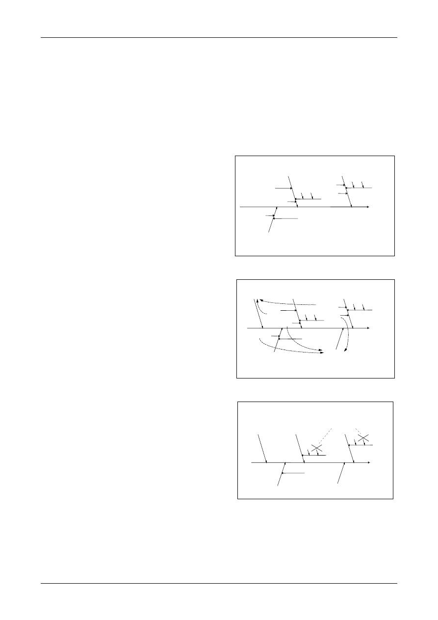
Quantifying Uncertainty

Appendix D – Analysing Uncertainty Sources

QUAM:2000.1

Page 101

density bottle; either could form the initial
structure. In practice this does not affect the
utility of the method. Provided that all significant
effects appear once, somewhere in the list, the
overall methodology remains effective.

D.3.4 Once the cause-and-effect analysis is
complete, it may be appropriate to return to the
original equation for the result and add any new
terms (such as temperature) to the equation.

D.4 Example

D.4.1 The procedure is illustrated by reference to
a simplified direct density measurement.
Consider the case of direct determination of the
density d(EtOH) of ethanol by weighing a known
volume V in a suitable volumetric vessel of tare
weight m

tare

and gross weight including ethanol

gross

. The density is calculated from

d(EtOH)=(m

gross

- m

tare

)/V

For clarity, only three effects will be considered:
Equipment calibration, Temperature, and the
precision of each determination. Figures D1-D3
illustrate the process graphically.

D.4.2 A cause and effect diagram consists of a
hierarchical structure culminating in a single
outcome. For the present purpose, this outcome
is a particular analytical result (‘

d(EtOH)

’ in

Figure D1). The ‘branches’ leading to the
outcome are the contributory effects, which
include both the results of particular intermediate
measurements and other factors, such as
environmental or matrix effects. Each branch
may in turn have further contributory effects.
These ‘effects’ comprise all factors affecting the
result, whether variable or constant; uncertainties
in any of these effects will clearly contribute to
uncertainty in the result.

D.4.3 Figure

D1 shows a possible diagram

obtained directly from application of steps 1-3.
The main branches are the parameters in the
equation, and effects on each are represented by
subsidiary branches. Note that there are two
‘temperature’ effects, three ‘precision’ effects
and three ‘calibration’ effects.

D.4.4 Figure D2

shows

precision

and

temperature effects each grouped together
following the second rule (same effect/time);
temperature may be treated as a single effect on
density, while the individual variations in each
determination contribute to variation observed in
replication of the entire method.

D.4.5 The calibration bias on the two weighings
cancels, and can be removed (Figure D3)
following the first refinement rule (cancellation).

D.4.6

Finally, the remaining ‘calibration’

branches would need to be distinguished as two
(different) contributions owing to possible non-
linearity of balance response, together with the
calibration uncertainty associated with the
volumetric determination.

Figure D1: Initial list

d(EtOH)

m(gross)

m(tare)

Volume

Temperature

Calibration

Precision

Calibration

Lin*. Bias

Precision

*Lin. = Linearity

Figure D2: Combination of similar effects

d(EtOH)

m(gross)

m(tare)

Volume

Temperature

Calibration

Precision

Calibration

Lin. Bias

Precision

Temperature

Figure D3: Cancellation

d(EtOH)

m(gross)

m(tare)

Volume

Calibration

Lin. Bias

Precision

Temperature

Same balance:

bias cancels

Quantifying Uncertainty

Appendix E – Statistical Procedures

QUAM:2000.1

Page 102

Appendix E. Useful Statistical Procedures

E.1 Distribution functions

The following table shows how to calculate a standard uncertainty from the parameters of the two most
important distribution functions, and gives an indication of the circumstances in which each should be used.

EXAMPLE

A chemist estimates a contributory factor as not less than 7 or more than 10, but feels that the value could be
anywhere in between, with no idea of whether any part of the range is more likely than another. This is a
description of a rectangular distribution function with a range 2a=3 (semi range of a=1

5). Using the function

below for a rectangular distribution, an estimate of the standard uncertainty can be calculated. Using the above
range, a=1

5, results in a standard uncertainty of (1.5/

√

3) = 0

87.

Rectangular distribution

Form

Use when:

Uncertainty

2a ( =

a )

1/2a

•

A certificate or other specification gives

limits without specifying a level of
confidence (e.g. 25ml

0.05ml)

•

An estimate is made in the form of a

maximum range (

a) with no knowledge

of the shape of the distribution.

)

(

Triangular distribution

Form

Use when:

Uncertainty

2a ( =

a )

1/a

•

The available information concerning x is

less limited than for a rectangular
distribution. Values close to x are more
likely than near the bounds.

•

An estimate is made in the form of a

maximum range (

a) described by a

symmetric distribution.

)

(

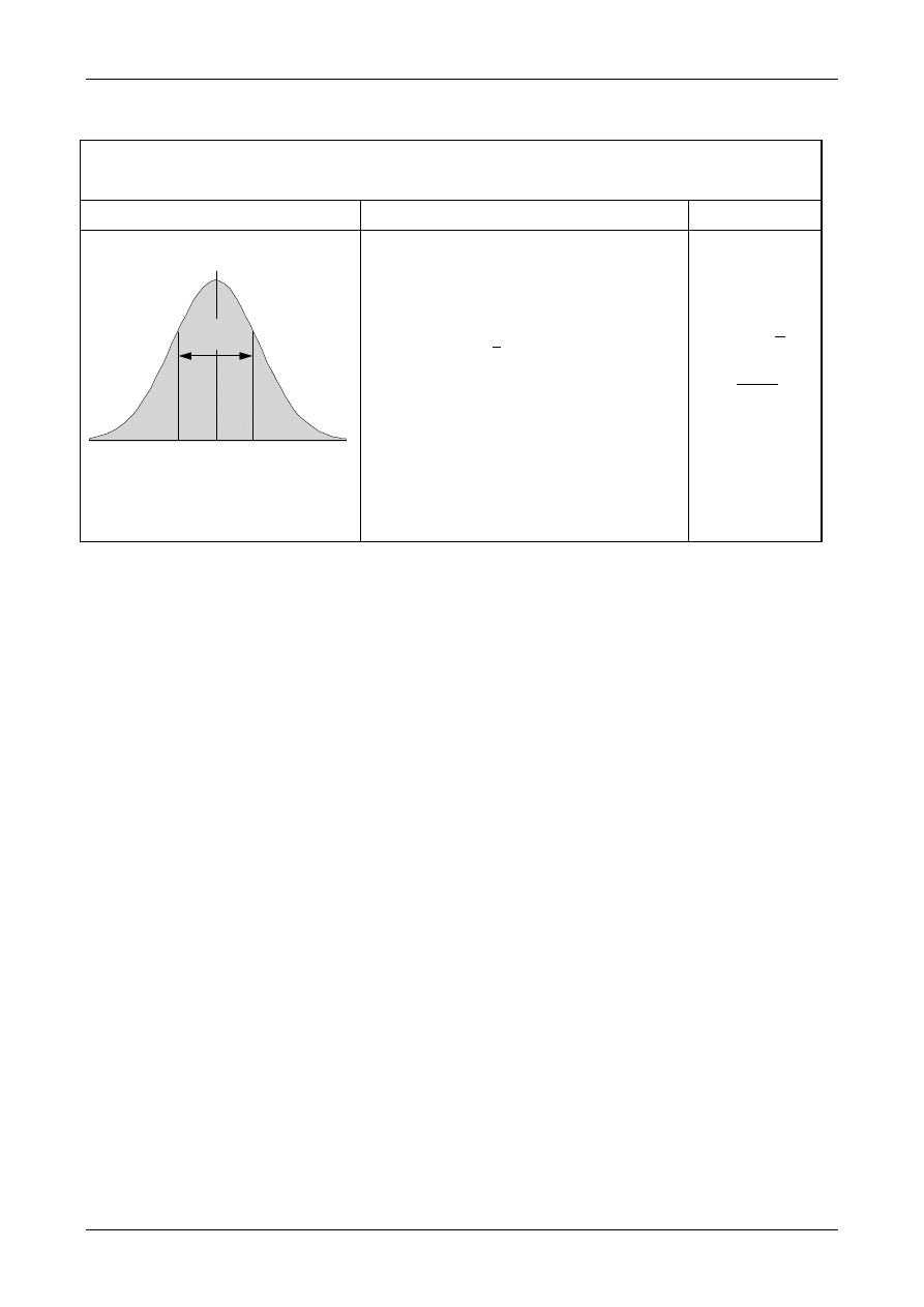
Quantifying Uncertainty

Appendix E – Statistical Procedures

QUAM:2000.1

Page 103

Normal distribution

Form

Use when:

Uncertainty

! An estimate is made from repeated

observations of a randomly varying
process.

u(x) = s

•

An uncertainty is given in the form of a

standard deviation s, a relative standard
deviation

s /

, or a coefficient of

variance CV% without specifying the
distribution.

u(x) = s

u(x)=x

⋅

(

s x

)

u(x)=

⋅

100

•

An uncertainty is given in the form of a

95% (or other) confidence interval

without specifying the distribution.

u(x) = c /2
(for

c at 95%)

u(x) = c/3
(for

c at 99.7%)

Quantifying Uncertainty

Appendix E – Statistical Procedures

QUAM:2000.1

Page 104

E.2 Spreadsheet method for uncertainty calculation

E.2.1 Spreadsheet software can be used to
simplify the calculations shown in Section 8. The
procedure takes advantage of an approximate
numerical method of differentiation, and requires
knowledge only of the calculation used to derive
the final result (including any necessary
correction factors or influences) and of the
numerical values of the parameters and their
uncertainties. The description here follows that of
Kragten [H.12].

E.2.2 In the expression for u(y(x

, x

...x

))

∑















⋅

∂

⋅

∂















⋅

∂

)

(

)

(

provided that either

y(x

...

) is linear in

u(x

) is small compared to

, the partial

differentials (

∂

) can be approximated by:

)

(

)

(

))

(

−

≈

∂

Multiplying by

u(x

) to obtain the uncertainty

u(y,x

) in

y due to the uncertainty in x

gives

u(y,x

)

≈

y(x

,..(x

+u(x

))

..x

)

-y(x

,..x

..x

)

Thus

u(y,x

) is just the difference between the

values of

y calculated for [x

u(x

)] and

respectively.

E.2.3 The assumption of linearity or small values
of

u(x

will not be closely met in all cases.

Nonetheless, the method does provide acceptable
accuracy for practical purposes when considered
against the necessary approximations made in
estimating the values of

u(x

). Reference H.12

discusses the point more fully and suggests
methods of checking the validity of the
assumption.

E.2.4 The basic spreadsheet is set up as follows,
assuming that the result

y is a function of the four

parameters

p, q, r, and s:

i) Enter the values of

p, q, etc. and the formula

for calculating

y in column A of the

spreadsheet. Copy column A across the
following columns once for every variable in

(see Figure E2.1). It is convenient to place the
values of the uncertainties

u(p), u(q) and so on

in row 1 as shown.

ii) Add

u(p) to p in cell B3, u(q) to q in cell C4

etc., as in Figure E2.2. On recalculating the
spreadsheet, cell B8 then becomes

f(p+u(p), q ,r..) (denoted by f (p’, q, r, ..) in
Figures E2.2 and E2.3), cell C8 becomes
f(p, q+u(q), r,..) etc.

iii) In row 9 enter row 8 minus A8 (for example,

cell B9 becomes B8-A8). This gives the values
of

u(y,p) as

u(y,p)=f (p+u(p), q, r ..) - f (p,q,r ..) etc.

iv) To obtain the standard uncertainty on

y, these

individual contributions are squared, added
together and then the square root taken, by
entering

u(y,p)

in row 10 (Figure E2.3) and

putting the square root of their sum in A10.
That is, cell A10 is set to the formula

SQRT(SUM(B10+C10+D10+E10))

which gives the standard uncertainty on

E.2.5 The contents of the cells B10, C10 etc.
show the squared contributions u(y,x

)

u(x

))

of the individual uncertainty components to the
uncertainty on

y and hence it is easy to see which

components are significant.

E.2.6

It is straightforward to allow updated

calculations as individual parameter values
change or uncertainties are refined. In step i)
above, rather than copying column A directly to
columns B-E, copy the values p to s by reference,
that is, cells B3 to E3 all reference A3, B4 to E4
reference A4

etc. The horizontal arrows in Figure

E2.1 show the referencing for row 3. Note that
cells B8 to E8 should still reference the values in
columns B to E respectively, as shown for column
B by the vertical arrows in Figure E2.1. In step ii)
above, add the references to row 1 by reference
(as shown by the arrows in Figure E2.1). For
example, cell B3 becomes A3+B1, cell C4
becomes A4+C1

etc. Changes to either

parameters or uncertainties will then be reflected
immediately in the overall result at A8 and the
combined standard uncertainty at A10.

E.2.7 If any of the variables are correlated, the
necessary additional term is added to the SUM in
A10. For example, if

p and q are correlated, with

a correlation coefficient

r(p,q), then the extra term

r(p,q)

u(y,p)

u(y,q) is added to the calculated

sum before taking the square root. Correlation can
therefore easily be included by adding suitable
extra terms to the spreadsheet.

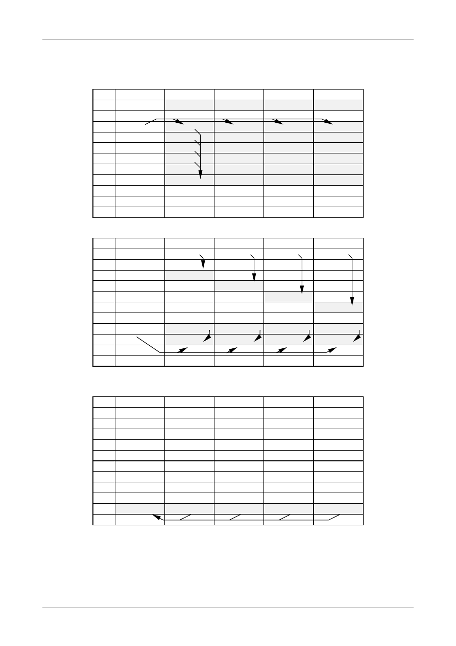
Quantifying Uncertainty

Appendix E – Statistical Procedures

QUAM:2000.1

Page 105

Figure E2.1

u(p)

u(q)

u(r)

u(s)

2
3

7
8

y=f(p,q,..)

9
10
11

Figure E2.2

u(p)

u(q)

u(r)

u(s)

2
3

p+u(p)

q+u(q)

r+u(r)

s+u(s)

7
8

y=f(p,q,..)

y=f(p’,...)

y=f(..q’,..)

y=f(..r’,..)

y=f(..s’,..)

u(y,p)

u(y,q)

u(y,r)

u(y,s)

10
11

Figure E2.3

u(p)

u(q)

u(r)

u(s)

2
3

p+u(p)

q+u(q)

r+u(r)

s+u(s)

7
8

y=f(p,q,..)

y=f(p’,...)

y=f(..q’,..)

y=f(..r’,..)

y=f(..s’,..)

u(y,p)

u(y,q)

u(y,r)

u(y,s)

u(y)

u(y,p)

u(y,q)

u(y,r)

u(y,s)

Quantifying Uncertainty

Appendix E – Statistical Procedures

QUAM:2000.1

Page 106

E.3 Uncertainties from linear least squares calibration

E.3.1 An analytical method or instrument is often
calibrated by observing the responses,

y, to

different levels of the analyte,

x. In most cases

this relationship is taken to be linear viz:

y = b

+ b

Eq.

E3.1

This calibration line is then used to obtain the
concentration

pred

of the analyte from a sample

which produces an observed response

obs

from

pred

= (

obs

–

Eq. E3.2

It is usual to determine the constants

and

weighted or un-weighted least squares regression
on a set of

n pairs of values (x

E.3.2 There are four main sources of uncertainty
to consider in arriving at an uncertainty on the
estimated concentration

pred

•

Random variations in measurement of y,

affecting both the reference responses

and

the measured response

obs

•

Random effects resulting in errors in the

assigned reference values

•

Values of x

and

may be subject to a

constant unknown offset, for example arising
when the values of

x are obtained from serial

dilution of a stock solution

•

The assumption of linearity may not be valid

Of these, the most significant for normal practice
are random variations in

y, and methods of

estimating uncertainty for this source are detailed
here. The remaining sources are also considered
briefly to give an indication of methods available.

E.3.3 The uncertainty u(x

pred

y) in a predicted

value

pred

due to variability in

y can be estimated

in several ways:

From calculated variance and covariance.

If the values of

and

, their variances var(

var(

) and their covariance, covar(

), are

determined by the method of least squares, the
variance on

x, var(x), obtained using the formula

in Chapter 8. and differentiating the normal
equations, is given by

)

var(

)

(

covar

)

var(

)

var(

)

var(

pred

obs

pred

⋅

Eq. E3.3

and the corresponding uncertainty

u(x

pred

y) is

√

var(

pred

From the calibration data.

The above formula for var(

pred

)

can be written in

terms of the set of

n data points, (x

), used to

determine the calibration function:















∑

−

∑

⋅

−

∑

⋅

)

(

)

(

)

(

)

var(

)

var(

pred

obs

pred

Eq. E3.4

where

)

(

)

(

−

∑

, )

(

−

is the

residual for the

point,

n is the number of data

points in the calibration,

the calculated best fit

gradient,

the weight assigned to

and

)

(

pred

−

the difference between

pred

and the

mean

x of the n values x

....

For unweighted data and where var(

obs

) is based

p measurements, equation E3.4 becomes















∑

−

∑

−

⋅

)

(

)

(

)

(

)

var(

pred

Eq. E3.5

This is the formula which is used in example 5

with

(

)

[

]

∑

−

)

(

)

(

From information given by software used to
derive calibration curves.

Some software gives the value of

S, variously

described for example as RMS error or residual
standard error. This can then be used in equation
E3.4 or E3.5. However some software may also
give the standard deviation

s(y

) on a value of y

calculated from the fitted line for some new value
of

x and this can be used to calculate var(x

pred

)

since, for

p=1

(

)

(

)

∑

−

pred

)

(

)

(

)

(

Quantifying Uncertainty

Appendix E – Statistical Procedures

QUAM:2000.1

Page 107

giving, on comparison with equation E3.5,

var(x

pred

) = [ s(y

) /

]

Eq. E3.6

E.3.4 The reference values x

may each have

uncertainties which propagate through to the final
result. In practice, uncertainties in these values
are usually small compared to uncertainties in the
system responses y

, and may be ignored. An

approximate estimate of the uncertainty u(x

pred

, x

)

in a predicted value x

pred

due to uncertainty in a

particular reference value x

u(x

pred

, x

)

≈

u(x

)/n

Eq. E3.7

where n is the number of x

values used in the

calibration. This expression can be used to check
the significance of u(x

pred

, x

E.3.5 The uncertainty arising from the assumption
of a linear relationship between y and x is not
normally large enough to require an additional
estimate. Providing the residuals show that there
is no significant systematic deviation from this
assumed relationship, the uncertainty arising from
this assumption (in addition to that covered by the
resulting increase in y variance) can be taken to
be negligible. If the residuals show a systematic
trend then it may be necessary to include higher

terms in the calibration function. Methods of
calculating var(x) in these cases are given in
standard texts. It is also possible to make a
judgement based on the size of the systematic
trend.

E.3.6 The values of x and y may be subject to a
constant unknown offset (e.g. arising when the
values of x are obtained from serial dilution of a
stock solution which has an uncertainty on its
certified value). If the standard uncertainties on y
and x from these effects are u(y, const) and
u(x,

const), then the uncertainty on the

interpolated value x

pred

is given by:

u(x

pred

)

= u(x, const)

(u(y, const)/b

)

+ var(x)

Eq. E3.8

E.3.7 The four uncertainty components described
in E.3.2 can be calculated using equations
Eq. E3.3 to Eq. E3.8. The overall uncertainty
arising from calculation from a linear calibration
can then be calculated by combining these four
components in the normal way.

Quantifying Uncertainty

Appendix E – Statistical Procedures

QUAM:2000.1

Page 108

E.4: Documenting uncertainty dependent on analyte level

E.4.1 Introduction

E.4.1.1

It is often observed in chemical

measurement that, over a large range of analyte
levels, dominant contributions to the overall
uncertainty vary approximately proportionately to
the level of analyte, that is u(x)

∝

x. In such cases

it is often sensible to quote uncertainties as
relative standard deviations or, for example,
coefficient of variation (%CV).

E.4.1.2 Where the uncertainty is unaffected by
level, for example at low levels, or where a
relatively narrow range of analyte level is
involved, it is generally most sensible to quote an
absolute value for the uncertainty.

E.4.1.3

In some cases, both constant and

proportional effects are important. This section
sets out a general approach to recording
uncertainty information where variation of
uncertainty with analyte level is an issue and
reporting as a simple coefficient of variation is
inadequate.

E.4.2 Basis of approach

E.4.2.1

To allow for both proportionality of

uncertainty and the possibility of an essentially
constant value with level, the following general
expression is used:

)

(

)

(

⋅

[1]

where

u(x) is the combined standard uncertainty in the

result x (that is, the uncertainty expressed
as a standard deviation)

represents a constant contribution to the

overall uncertainty

is a proportionality constant.

The expression is based on the normal method of
combining of two contributions to overall
uncertainty, assuming one contribution (s

) is

constant and one (xs

) proportional to the result.

Figure E.4.1 shows the form of this expression.

OTE

: The approach above is practical only where it

is possible to calculate a large number of
values. Where experimental study is
employed, it will not often be possible to
establish the relevant parabolic relationship. In
such circumstances, an adequate

approximation can be obtained by simple
linear regression through four or more
combined uncertainties obtained at different
analyte concentrations. This procedure is
consistent with that employed in studies of
reproducibility and repeatability according to
ISO 5725:1994. The relevant expression is
then

u x

x s

( )

. '

≈

E.4.2.2 The figure can be divided into
approximate regions (A to C on the figure):

A: The uncertainty is dominated by the term s

and is approximately constant and close to s

B: Both terms contribute significantly; the

resulting uncertainty is significantly higher
than either s

or xs

, and some curvature is

visible.

C: The term xs

dominates; the uncertainty rises

approximately linearly with increasing x and
is close to xs

E.4.2.3 Note that in many experimental cases the
complete form of the curve will not be apparent.
Very often, the whole reporting range of analyte
level permitted by the scope of the method falls
within a single chart region; the result is a number
of special cases dealt with in more detail below.

E.4.3 Documenting level-dependent

uncertainty data

E.4.3.1

In general, uncertainties can be

documented in the form of a value for each of s

and s

. The values can be used to provide an

uncertainty estimate across the scope of the
method. This is particularly valuable when
calculations for well characterised methods are
implemented on computer systems, where the
general form of the equation can be implemented
independently of the values of the parameters
(one of which may be zero - see below). It is
accordingly recommended that, except in the
special cases outlined below or where the
dependence is strong but not linear

, uncertainties

An important example of non-linear dependence is

the effect of instrument noise on absorbance
measurement at high absorbances near the upper limit
of the instrument capability. This is particularly
pronounced where absorbance is calculated from
transmittance (as in infrared spectroscopy). Under
these circumstances, baseline noise causes very large
uncertainties in high absorbance figures, and the

Quantifying Uncertainty

Appendix E – Statistical Procedures

QUAM:2000.1

Page 109

are documented in the form of values for a
constant term represented by s

and a variable

term represented by s

E.4.4. Special cases

E.4.4.1. Uncertainty not dependent on level of
analyte (

dominant)

The uncertainty will generally be effectively
independent of observed analyte concentration
when:

•

The result is close to zero (for example,

within the stated detection limit for the
method). Region A in Figure E.4.1

•

The possible range of results (stated in the

method scope or in a statement of scope for
the uncertainty estimate) is small compared to
the observed level.

Under these circumstances, the value of s

can be

recorded as zero. s

is normally the calculated

standard uncertainty.

E.4.4.2. Uncertainty entirely dependent on
analyte (

dominant)

Where the result is far from zero (for example,
above a ‘limit of determination’) and there is
clear evidence that the uncertainty changes
proportionally with the level of analyte permitted
within the scope of the method, the term xs

dominates (see Region C in Figure E.4.1). Under
these circumstances, and where the method scope
does not include levels of analyte near zero, s

may reasonably be recorded as zero and s

simply the uncertainty expressed as a relative
standard deviation.

E.4.4.3. Intermediate dependence

In intermediate cases, and in particular where the
situation corresponds to region B in Figure E.4.1,
two approaches can be taken:

a) Applying variable dependence

The more general approach is to determine,
record and use both s

and s

. Uncertainty

uncertainty rises much faster than a simple linear
estimate would predict. The usual approach is to
reduce the absorbance, typically by dilution, to bring
the absorbance figures well within the working range;
the linear model used here will then normally be
adequate. Other examples include the ‘sigmoidal’
response of some immunoassay methods.

estimates, when required, can then be produced
on the basis of the reported result. This remains
the recommended approach where practical.

OTE

: See the note to section E.4.2.

b) Applying a fixed approximation

An alternative which may be used in general
testing and where

•

the dependence is not strong (that is,

evidence for proportionality is weak)

•

the range of results expected is moderate

leading in either case to uncertainties which do
not vary by more than about 15% from an
average uncertainty estimate, it will often be
reasonable to calculate and quote a fixed value of
uncertainty for general use, based on the mean
value of results expected. That is,

either

a mean or typical value for x is used to
calculate a fixed uncertainty estimate, and this
is used in place of individually calculated
estimates

a single standard deviation has been obtained,
based on studies of materials covering the full
range of analyte levels permitted (within the
scope of the uncertainty estimate), and there is
little evidence to justify an assumption of
proportionality. This should generally be
treated as a case of zero dependence, and the
relevant standard deviation recorded as s

E.4.5. Determining

and

E.4.5.1. In the special cases in which one term
dominates, it will normally be sufficient to use the
uncertainty as standard deviation or relative
standard deviation respectively as values of s

and

. Where the dependence is less obvious,

however, it may be necessary to determine s

and

indirectly from a series of estimates of

uncertainty at different analyte levels.

E.4.5.2. Given a calculation of combined
uncertainty from the various components, some of
which depend on analyte level while others do
not, it will normally be possible to investigate the
dependence of overall uncertainty on analyte level
by simulation. The procedure is as follows:

Quantifying Uncertainty

Appendix E – Statistical Procedures

QUAM:2000.1

Page 110

Calculate (or obtain experimentally)
uncertainties u(x

) for at least ten levels x

analyte, covering the full range permitted.

2. Plot

u(x

)

against x

3. By linear regression, obtain estimates of m

and c for the line u(x)

= mx

+ c

4. Calculate

and s

from s

√

c, s

√

5. Record

and s

E.4.6. Reporting

E.4.6.1. The approach outlined here permits
estimation of a standard uncertainty for any single
result. In principle, where uncertainty information
is to be reported, it will be in the form of

[result]

[uncertainty]

where the uncertainty as standard deviation is
calculated as above, and if necessary expanded
(usually by a factor of two) to give increased
confidence. Where a number of results are
reported together, however, it may be possible,
and is perfectly acceptable, to give an estimate of
uncertainty applicable to all results reported.

E.4.6.2. Table E.4.1 gives some examples. The
uncertainty figures for a list of different analytes
may usefully be tabulated following similar
principles.

OTE

: Where a ‘detection limit’ or ‘reporting limit’

is used to give results in the form “<x” or
“nd”, it will normally be necessary to quote
the limits used in addition to the uncertainties
applicable to results above reporting limits.

Table E.4.1: Summarising uncertainty for several samples

Situation

Dominant term

Reporting example(s)

Uncertainty essentially constant
across all results

or fixed approximation

(sections E.4.4.1. or E.4.4.3.a)

Standard deviation: expanded
uncertainty; 95% confidence
interval

Uncertainty generally
proportional to level

(see section E.4.4.2.)

relative standard deviation;
coefficient of variance (%CV)

Mixture of proportionality and
lower limiting value for
uncertainty

Intermediate case

(section E.4.4.3.)

quote %CV or rsd together with
lower limit as standard
deviation.

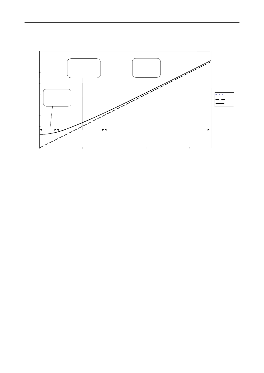
Quantifying Uncertainty

Appendix E – Statistical Procedures

QUAM:2000.1

Page 111

Figure E.4.1: Variation of uncertainty with observed result

0.2

0.4

0.6

0.8

1.2

1.4

1.6

1.8

Result x

Uncertainty u(x)

x.s

u(x)

Uncertainty

approximately

equal to s

Uncertainty
significantly

greater than

either s

or x.s

Uncertainty

approximately
equal to x.s

Quantifying Uncertainty

Appendix F – Detection limits

QUAM:2000.1

Page 112

Appendix F. Measurement Uncertainty at the Limit of Detection/Limit of

Determination

F.1. Introduction

F.1.1.

At low concentrations, an increasing

variety of effects becomes important, including,
for example,

•

the presence of noise or unstable baseline,

•

the contribution of interferences to the (gross)

signal,

•

the influence of any analytical blank used,

and

•

losses during extraction, isolation or clean-up.

Because of such effects, as analyte concentrations
drop, the relative uncertainty associated with the
result tends to increase, first to a substantial
fraction of the result and finally to the point
where the (symmetric) uncertainty interval
includes zero. This region is typically associated
with the practical limit of detection for a given
method.

OTE

: The terminology and conventions associated

with measuring and reporting low levels of
analyte have been widely discussed elsewhere
(See Bibliography [H.16, H.17, H.18] for
examples and definitions). Here, the term
‘limit of detection’ only implies a level at
which detection becomes problematic, and is
not associated with any specific definition.

F.1.2.

It is widely accepted that the most

important use of the ‘limit of detection’ is to show
where method performance becomes insufficient
for acceptable quantitation, so that improvements
can be made. Ideally, therefore, quantitative
measurements should not be made in this region.
Nonetheless, so many materials are important at
very low levels that it is inevitable that
measurements must be made, and results reported,
in this region.

F.1.3.

The ISO Guide on Measurement

Uncertainty [H.2] does not give explicit
instructions for the estimation of uncertainty
when the results are small and the uncertainties
large compared to the results. Indeed, the basic
form of the ‘law of propagation of uncertainties’,
described in chapter 8 of this guide, may cease to
apply accurately in this region; one assumption on
which the calculation is based is that the

uncertainty is small relative to the value of the
measurand. An additional, if philosophical,
difficulty follows from the definition of
uncertainty given by the ISO Guide: though
negative observations are quite possible, and even
common in this region, an implied dispersion
including values below zero cannot be “...
reasonably ascribed to the value of the
measurand” when the measurand is a
concentration, because concentrations themselves
cannot be negative.

F.1.4.

These difficulties do not preclude the

application of the methods outlined in this guide,
but some caution is required in interpretation and
reporting the results of measurement uncertainty
estimation in this region. The purpose of the
present Appendix is to provide limited guidance
to supplement that already available from other
sources.

OTE

: Similar considerations may apply to other

regions; for example, mole or mass fractions
close to 100% may lead to similar difficulties.

F.2. Observations and estimates

F.2.1. A fundamental principle of measurement
science is that results are estimates of true values.
Analytical results, for example, are available
initially in units of the observed signal, e.g. mV,
absorbance units etc. For communication to a
wider audience, particularly to the customers of a
laboratory or to other authorities, the raw data
need to be converted to a chemical quantity, such
as concentration or amount of substance. This
conversion typically requires a calibration
procedure (which may include, for example,
corrections for observed and well characterised
losses). Whatever the conversion, however, the
figure generated remains an observation, or
signal. If the experiment is properly carried out,
this observation remains the ‘best estimate’ of the
value of the measurand.

F.2.2. Observations are not often constrained by
the same fundamental limits that apply to real
concentrations. For example, it is perfectly
sensible to report an ‘observed concentration’,

Quantifying Uncertainty

Appendix F – Detection limits

QUAM:2000.1

Page 113

that is, an estimate, below zero. It is equally
sensible to speak of a dispersion of possible
observations which extends into the same region.
For example, when performing an unbiased
measurement on a sample with no analyte present,
one should see about half of the observations
falling below zero. In other words, reports like

observed concentration = 2.4

8 mg l

-1

observed concentration = -4.2

8 mg l

-1

are not only possible; they should be seen as
valid statements.

F.2.3.

The methods of uncertainty estimation

described in this guide apply well to the
estimation of uncertainties on observations. It
follows that while reporting observations and
their associated uncertainties to an informed
audience, there is no barrier to, or contradiction
in, reporting the best estimate and its associated
uncertainty even where the result implies an
impossible physical situation. Indeed, in some
circumstances (for example, when reporting a
value for an analytical blank which will
subsequently be used to correct other results) it is
absolutely essential to report the observation and
its uncertainty (however large).

F.2.4. This remains true wherever the end use of
the result is in doubt. Since only the observation
and its associated uncertainty can be used directly
(for example, in further calculations, in trend
analysis or for re-interpretation), the uncensored
observation should always be available.

F.2.5. The ideal is accordingly to report valid
observations and their associated uncertainty
regardless of the values.

F.3. Interpreted results and compliance

statements

F.3.1. Despite the foregoing, it must be accepted
that many reports of analysis and statements of
compliance include some interpretation for the
end user’s benefit. Typically, such an
interpretation would include any relevant
inference about the levels of analyte which could
reasonably be present in a material. Such an
interpretation is an inference about the real world,
and consequently would be expected (by the end
user) to conform to real limits. So, too, would any
associated estimate of uncertainty in ‘real’ values.

F.3.2. Under such circumstances, where the end
use is well understood, and where the end user
cannot realistically be informed of the nature of
measurement observations, the general guidance
provided elsewhere (for example in references
H.16, H.17, H.18) on the reporting of low level
results may reasonably apply.

F.3.3. One further caution is, however, pertinent.
Much of the literature on capabilities of detection
relies heavily on the statistics of repeated
observations. It should be clear to readers of the
current guide that observed variation is only
rarely a good guide to the full uncertainty of
results. Just as with results in any other region,
careful consideration should accordingly be given
to all the uncertainties affecting a given result
before reporting the values.

Quantifying Uncertainty

Appendix G – Uncertainty Sources

QUAM:2000.1

Page 114

Appendix G. Common Sources and Values of Uncertainty

The following tables summarise some typical examples of uncertainty components. The
tables give:

•

The particular measurand or experimental procedure (determining mass, volume
etc)

•

The main components and sources of uncertainty in each case

•

A suggested method of determining the uncertainty arising from each source.

•

An example of a typical case

The tables are intended only to summarise the examples and to indicate general methods
of estimating uncertainties in analysis. They are not intended to be comprehensive, nor
should the values given be used directly without independent justification. The values
may, however, help in deciding whether a particular component is significant.

Determination

Uncertainty

Cause

Method of determination

Typical values

Components

Example

Value

Mass

Balance calibration

uncertainty

Limited accuracy in

calibration

Stated on calibration certificate,

converted to standard deviation

4-figure balance

0.5 mg

Linearity

i) Experiment, with range of

certified weights

ii) Manufacturer's specification

ca. 0.5x last

significant digit

Readability

Limited resolution on

display or scale

From last significant digit

0.5x last

significant

digit/

√

Daily drift

Various, including

temperature

Standard deviation of long term

check weighings. Calculate as

RSD if necessary.

ca. 0.5x last

significant

digit.

Run to run variation

Various

Standard deviation of successive

sample or check weighings

ca. 0.5x last

significant

digit.

Density effects

(conventional

basis)

Note

Calibration weight/sample

density mismatch causes a

difference in the effect of

atmospheric buoyancy

Calculated from known or

assumed densities and typical

atmospheric conditions

Steel, Nickel

Aluminium

Organic solids

Water

Hydrocarbons

1 ppm

20 ppm

50-100 ppm

65 ppm

90 ppm

Density effects

(in vacuo

basis)

Note 1

As above.

Calculate atmospheric buoyancy

effect and subtract buoyancy

effect on calibration weight.

100 g water

g Nickel

+0.1g (effect)

<1 mg (effect)

Note 1. For fundamental constants or SI unit definitions, mass determinations by weighing are usually corrected to the weight in vacuum. In most other practical

situations, weight is quoted on a

conventional

basis as defined by OIML [H.18]. The convention is to quote weights at an air density of 1.2

-3

and a sample

density of 8000

-3

, which corresponds to weighing steel at sea level in normal atmospheric conditions. The buoyancy correction to conventional mass is zero

when the sample density is 8000

-3

or the air density is 1.2

-3

. Since the air density is usually very close to the latter value, correction to conventional weight

can normally be neglected. The standard uncertainty values given for density-related effects on a conventional weight basis in the table above are sufficient for

preliminary estimates for weighing on a conventional basis without buoyancy correction at sea level. Mass determined on the conventional basis may, however,

differ from the ‘true mass’ (

vacuo

) by 0.1% or more (see the effects in the bottom line of the table above).

QUAM:2000.1

Page 115

Quantifying Uncertainty

Appendix G – Uncertainty Sources

* Assuming rectangular

distribution

Determination

Uncertainty

Cause

Method of determination

Typical values

Components

Example

Value

Volume (liquid)

Calibration uncertainty

Limited accuracy in

calibration

Stated on manufacturer's

specification, converted to

standard deviation.

For ASTM class A glassware of

volume V, the limit is

approximately V

0.6

/200

ml (Grade A)

0.02 /

√

3 =

0.01 ml*

Temperature

Temperature variation

from the calibration

temperature causes a

difference in the volume

at the standard

temperature.

∆

⋅α

/(2

√

3) gives the relative

standard deviation, where

∆

T is

the possible temperature range

and

the coefficient of volume

expansion of the liquid.

approximately 2 x10

-4

-1

for

water and 1 x 10

-3

-1

for

organic liquids.

100

ml water

0.03 ml for

operating

within 3

C of

the stated

operating

temperature

Run to run variation

Various

Standard deviation of successive

check deliveries (found by

weighing)

25 ml pipette

Replicate

fill/weigh:

0.0092

QUAM:2000.1

Page 116

Quantifying Uncertainty

Appendix G – Uncertainty Sources

Determination

Uncertainty

Cause

Method of determination

Typical values

Components

Example

Value

Reference material

concentration

Purity

Impurities reduce the

amount of reference

material present. Reactive

impurities may interfere

with the measurement.

Stated on manufacturer’s

certificate. Reference certificates

usually give unqualified limits;

these should accordingly be

treated as rectangular

distributions and divided by

√

Note: where the nature of the

impurities is not stated, additional

allowance or checks may need to

be made to establish limits for

interference etc.

Reference

potassium

hydrogen

phthalate

certified as 99.9

0.1%

0.1/

√

3 =

0.06%

Concentration

(certified)

Certified uncertainty in

reference material

concentration.

Stated on manufacturer’s

certificate. Reference certificates

usually give unqualified limits;

these should accordingly be

treated as rectangular

distributions and divided by

√

Cadmium

acetate in 4%

acetic acid.

Certified as

(1000

-1

√

3 = 1.2

-1

(0.0012 as

RSD)*

Concentration (made

up from certified

material)

Combination of

uncertainties in reference

values and intermediate

steps

Combine values for prior steps as

RSD throughout.

Cadmium

acetate after

three dilutions

from 1000 mg

-1

to 0.5

-1

0034.

0017.

0021.

0017.

0012.

as RSD

*Assuming rectangular distribution

QUAM:2000.1

Page 117

Quantifying Uncertainty

Appendix G – Uncertainty Sources

Determination

Uncertainty

Cause

Method of determination

Typical values

Components

Example

Value

Absorbance

Instrument calibration

Note: this component

relates to absorbance

reading versus

reference absorbance,

not to the calibration of

concentration against

absorbance reading

Limited accuracy in

calibration.

Stated on calibration certificate as

limits, converted to standard

deviation

Run to run variation

Various

Standard deviation of replicate

determinations, or QA

performance.

Mean of 7

absorbance

readings with

s=1.63

1.63/

√

7 = 0.62

Sampling

Homogeneity

Sub-sampling from

inhomogeneous material

will not generally

represent the bulk exactly.

Note: random sampling

will generally result in zero

bias. It may be necessary

to check that sampling is

actually random.

i) Standard deviation of separate

sub-sample results (if the

inhomogeneity is large relative to

analytical accuracy).

ii) Standard deviation estimated

from known or assumed

population parameters.

Sampling from

bread of

assumed two-

valued

inhomogeneity

(See Example

A4)

For 15 portions

from 72

contaminated

and 360

uncontaminated

bulk portions:

RSD = 0.58

QUAM:2000.1

Page 118

Quantifying Uncertainty

Appendix G – Uncertainty Sources

Determination

Uncertainty

Cause

Method of determination

Typical values

Components

Example

Value

Extraction recovery

Mean recovery

Extraction is rarely

complete and may add or

include interferents.

Recovery calculated as

percentage recovery from

comparable reference material

or representative spiking.

Uncertainty obtained from

standard deviation of mean of

recovery experiments.

Note: recovery may also be

calculated directly from

previously measured partition

coefficients.

Recovery of

pesticide from

bread; 42

experiments,

mean 90%,

s=28%

(See Example

A4)

28/

√

42= 4.3%

(0.048 as

RSD)

Run to run variation in

recovery

Various

Standard deviation of replicate

experiments.

Recovery of

pesticides from

bread from

paired replicate

data. (See

Example A4)

0.31 as RSD.

QUAM:2000.1

Page 119

Quantifying Uncertainty

Appendix G – Uncertainty Sources

Quantifying Uncertainty

Appendix H - Bibliography

QUAM:2000.1

Page 120

Appendix H. Bibliography

H.1. ISO/IEC 17025:1999. General Requirements for the Competence of Calibration and Testing

Laboratories. ISO, Geneva (1999).

H.2. Guide To The Expression Of Uncertainty In Measurement. ISO, Geneva (1993).

(ISBN 92-67-10188-9) (Reprinted 1995)

H.3. EURACHEM, Quantifying Uncertainty in Analytical Measurement. Laboratory of the

Government Chemist, London (1995). ISBN 0-948926-08-2

H.4. International Vocabulary of basic and general terms in Metrology. ISO, Geneva, (1993). (ISBN

92-67-10175-1)

H.5. ISO 3534:1993. Statistics - Vocabulary and Symbols. ISO, Geneva, Switzerland (1993).

H.6. Analytical Methods Committee, Analyst (London).

120 29-34 (1995).

H.7. EURACHEM, The Fitness for Purpose of Analytical Methods. (1998) (ISBN 0-948926-12-0)

H.8. ISO/IEC Guide 33:1989, “Uses of Certified Reference Materials”. ISO, Geneva (1989).

H.9. International Union of Pure and Applied Chemistry. Pure Appl. Chem.,

67, 331-343, (1995).

H.10 ISO 5725:1994 (Parts 1-4 and 6). “Accuracy (trueness and precision) of measurement methods

and results”. ISO, Geneva (1994). See also ISO 5725-5:1998 for alternative methods of
estimating precision.

H.11. I. J. Good, "Degree of Belief", in Encyclopaedia of Statistical Sciences, Vol. 2, Wiley, New York

(1982).

H.12. J. Kragten, “Calculating standard deviations and confidence intervals with a universally

applicable spreadsheet technique”, Analyst,

119, 2161-2166 (1994).

H.13. British Standard BS 6748:1986. Limits of metal release from ceramic ware, glassware, glass

ceramic ware and vitreous enamel ware.

H.14. S. L. R. Ellison, V. J. Barwick. Accred. Qual. Assur.

3 101-105 (1998).

H.15. ISO 9004-4:1993, Total Quality Management. Part 2. Guidelines for quality improvement. ISO,

Geneva (1993).

H.16. H. Kaiser, Anal. Chem.

42 24A (1970).

H.17. L.A. Currie, Anal. Chem.

40 583 (1968).

H.18. IUPAC, Limit of Detection, Spectrochim. Acta

33B 242 (1978).

H.19. OIML Recommendations IR 33 Conventional value of the result of weighing in air.



2000

ISBN 0 948926 15 5

Wyszukiwarka

Podobne podstrony:
Laboratorium niepewność pomiarów analitycznych
NIEPEWNOŚĆ POMIARU
Wyk%c5%82ad Niepewno%c5%9b%c4%87 pomiaru
mierniki i niepewności pomiarowe
Błąd i niepewność pomiaru
podstawy analizy niepewności pomiarowych
Wyznaczanie niepewności pomiarów, PWr W9 Energetyka stopień inż, II Semestr, Podstawy metrologii i t
niepewnosci pomiarowe
3 Wyznaczanie niepewności pomiaru pośredniego
00 niepewność pomiaru
F2- Obliczenia i rachunek niepewności pomiarowej, Szkoła, Fizyka 02
niepewnosci pomiarowe, PWr, SEMESTR 1, FIZYKA, sprawozdania

więcej podobnych podstron