Lecture Notes: Introduction to Finite Element Method

Chapter 2. Bar and Beam Elements

© 1998 Yijun Liu, University of Cincinnati

25

Chapter 2. Bar and Beam Elements.

Linear Static Analysis

I. Linear Static Analysis

Most structural analysis problems can be treated as linear

static problems, based on the following assumptions

1. Small deformations (loading pattern is not changed due

to the deformed shape)

2. Elastic materials (no plasticity or failures)

3. Static loads (the load is applied to the structure in a slow

or steady fashion)

Linear analysis can provide most of the information about

the behavior of a structure, and can be a good approximation for
many analyses. It is also the bases of nonlinear analysis in most
of the cases.

Lecture Notes: Introduction to Finite Element Method

Chapter 2. Bar and Beam Elements

© 1998 Yijun Liu, University of Cincinnati

26

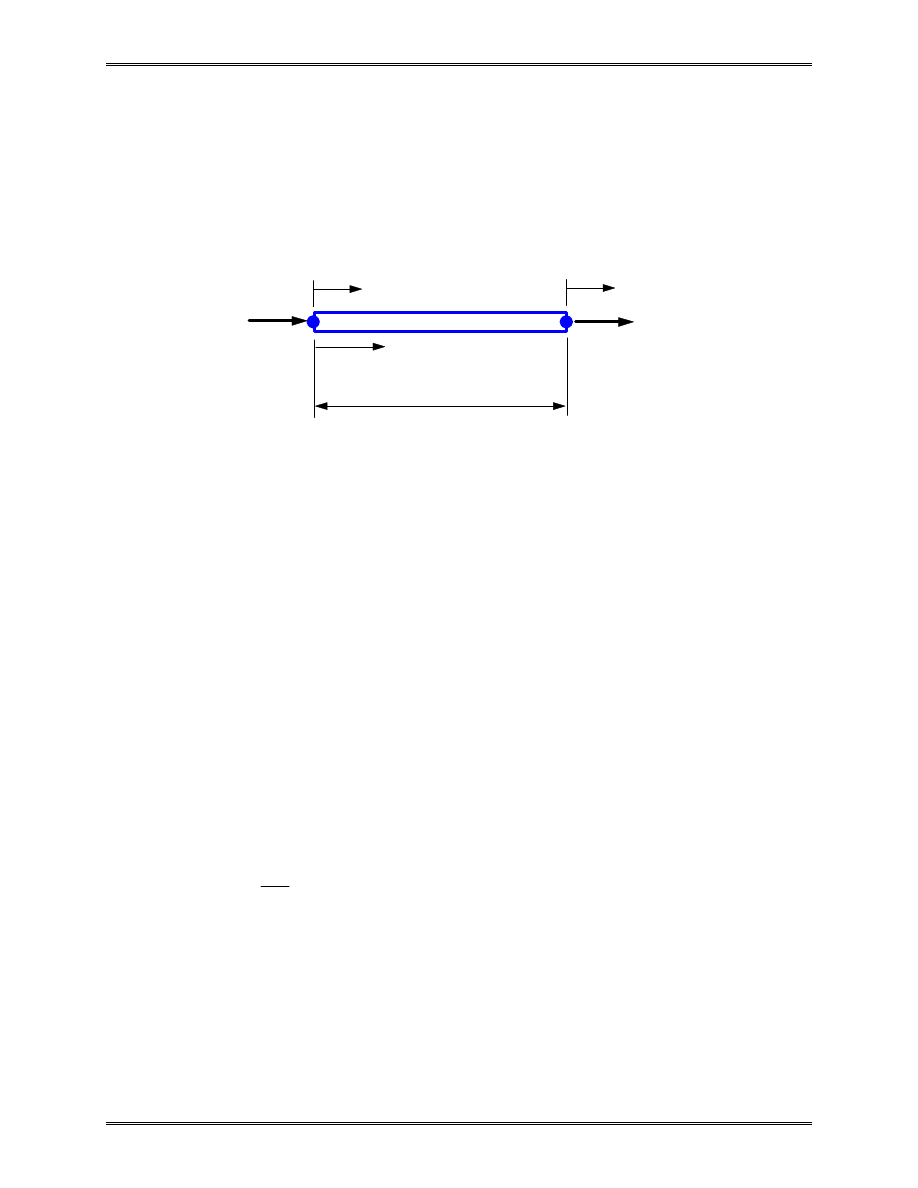
II. Bar Element

Consider a uniform prismatic bar:

L

length

A

cross-sectional area

E

elastic modulus

u

u x

=

( )

displacement

ε ε

=

( )

x

strain

σ σ

=

( )

x

stress

Strain-displacement relation:

ε

=

du

dx

(1)

Stress-strain relation:

σ

ε

=

E

(2)

L

x

f

i

i

j

f

j

u

i

u

j

A,E

Lecture Notes: Introduction to Finite Element Method

Chapter 2. Bar and Beam Elements

© 1998 Yijun Liu, University of Cincinnati

27

Stiffness Matrix --- Direct Method

Assuming that the displacement u is varying linearly along

the axis of the bar, i.e.,

u x

x

L

u

x

L

u

i

j

( )

= −







 +

1

(3)

we have

ε

=

−

=

u

u

L

L

j

i

∆

(

∆

= elongation)

(4)

σ

ε

=

=

E

E

L

∆

(5)

We also have

σ

=

F

A

(F = force in bar)

(6)

Thus, (5) and (6) lead to

F

EA

L

k

=

=

∆

∆

(7)

where

k

EA

L

=

is the stiffness of the bar.

The bar is acting like a spring in this case and we conclude

that element stiffness matrix is

Lecture Notes: Introduction to Finite Element Method

Chapter 2. Bar and Beam Elements

© 1998 Yijun Liu, University of Cincinnati

28

k

=

−

−







=

−

−





















k

k

k

k

EA

L

EA

L

EA

L

EA

L

or

k

=

−

−







EA

L

1

1

1

1

(8)

This can be verified by considering the equilibrium of the forces
at the two nodes.

Element equilibrium equation is

EA

L

u

u

f

f

i

j

i

j

1

1

1

1

−

−



















=













(9)

Degree of Freedom (dof)

Number of components of the displacement vector at a

node.

For 1-D bar element: one dof at each node.

Physical Meaning of the Coefficients in k

The jth column of k (here j = 1 or 2) represents the forces

applied to the bar to maintain a deformed shape with unit
displacement at node j and zero displacement at the other node.

Lecture Notes: Introduction to Finite Element Method

Chapter 2. Bar and Beam Elements

© 1998 Yijun Liu, University of Cincinnati

29

Stiffness Matrix --- A Formal Approach

We derive the same stiffness matrix for the bar using a

formal approach which can be applied to many other more
complicated situations.

Define two linear shape functions as follows

N

N

i

j

( )

,

( )

ξ

ξ

ξ

ξ

= −

=

1

(10)

where

ξ

ξ

=

≤ ≤

x

L

,

0

1

(11)

From (3) we can write the displacement as

u x

u

N

u

N

u

i

i

j

j

( )

( )

( )

( )

=

=

+

ξ

ξ

ξ

or

[

]

u

N

N

u

u

i

j

i

j

=













=

Nu

(12)

Strain is given by (1) and (12) as

ε

=

= 






=

du

dx

d

dx

N u

Bu

(13)

where B is the element strain-displacement matrix, which is

[

] [

]

B

=

=

•

d

dx

N

N

d

d

N

N

d

dx

i

j

i

j

( )

( )

( )

( )

ξ

ξ

ξ

ξ

ξ

ξ

i.e.,

[

]

B

= −

1

1

/

/

L

L

(14)

Lecture Notes: Introduction to Finite Element Method

Chapter 2. Bar and Beam Elements

© 1998 Yijun Liu, University of Cincinnati

30

Stress can be written as

σ

ε

=

=

E

EBu

(15)

Consider the strain energy stored in the bar

(

)

(

)

U

dV

E

dV

E

dV

V

V

V

=

=

=

















∫

∫

∫

1

2

1

2

1

2

σ ε

T

T

T

T

T

u B

Bu

u

B

B

u

(16)

where (13) and (15) have been used.

The work done by the two nodal forces is

W

f u

f u

i

i

j

j

=

+

=

1

2

1

2

1

2

u f

T

(17)

For conservative system, we state that

U

W

=

(18)

which gives

(

)

1

2

1

2

u

B

B

u

u f

T

T

T

E

dV

V

∫

















=

We can conclude that

(

)

B

B

u

f

T

E

dV

V

∫

















=

or

Lecture Notes: Introduction to Finite Element Method

Chapter 2. Bar and Beam Elements

© 1998 Yijun Liu, University of Cincinnati

31

ku

f

=

(19)

where

(

)

k

B

B

T

=

∫

E

dV

V

(20)

is the element stiffness matrix.

Expression (20) is a general result which can be used for

the construction of other types of elements. This expression can
also be derived using other more rigorous approaches, such as
the Principle of Minimum Potential Energy, or the Galerkin’s
Method.

Now, we evaluate (20) for the bar element by using (14)

[

]

k

=

−













−

=

−

−







∫

1

1

1

1

1

1

1

1

0

/

/

/

/

L

L

E

L

L Adx

EA

L

L

which is the same as we derived using the direct method.

Note that from (16) and (20), the strain energy in the

element can be written as

U

=

1

2

u ku

T

(21)