Lecture 10: Introduction to Statistical Process Control

Spanos

EE290H F05

1

Introduction to Statistical Process Control

The assignable cause
The Control Chart
Statistical basis of the control chart
Control limits, false and true alarms and the

operating characteristic function

Lecture 10: Introduction to Statistical Process Control

Spanos

EE290H F05

2

Managing Variation over Time

• Statistical Process Control often takes the form

of a continuous Hypothesis testing.

• The idea is to detect, as quickly as possible, a

significant departure from the norm.

• A significant change is often attributed to what is

known as an assignable cause.

• An assignable cause is something that can be

discovered and corrected at the machine level.

Lecture 10: Introduction to Statistical Process Control

Spanos

EE290H F05

3

What is the Assignable Cause?

• An "Assignable Cause" relates to relatively strong

changes, outside the random pattern of the process.

• It is "Assignable", i.e. it can be discovered and corrected

at the machine level.

• Although the detection of an assignable cause can be

automated, its identification and correction often requires
intimate understanding of the manufacturing process.

• For example...

– Symptom: significant yield drop.
– Assignable Cause: leaky etcher load lock door seal.
– Symptom: increased e-test rejections
– Assignable Cause: probe card worn out.

Lecture 10: Introduction to Statistical Process Control

Spanos

EE290H F05

4

Example:

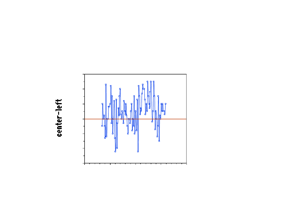
The pattern is obvious. How can we automate the alarm?

Investigate furnace temp and set up a real-time alarm.

20000

15000

10000

5000

0

-3

-2

-1

0

1

2

3

time

Lecture 10: Introduction to Statistical Process Control

Spanos

EE290H F05

5

The purpose of SPC

A. Detect the presence of an assignable cause fast.
2. Minimize needles adjustment.

• Like Hypothesis testing

– (A) means having low probability of type II error and
– (B) means having low probability of type I error.

• SPC needs a probabilistic model in order to describe the

process in question.

Lecture 10: Introduction to Statistical Process Control

Spanos

EE290H F05

6

Example: Furnace temp differential (cont.)

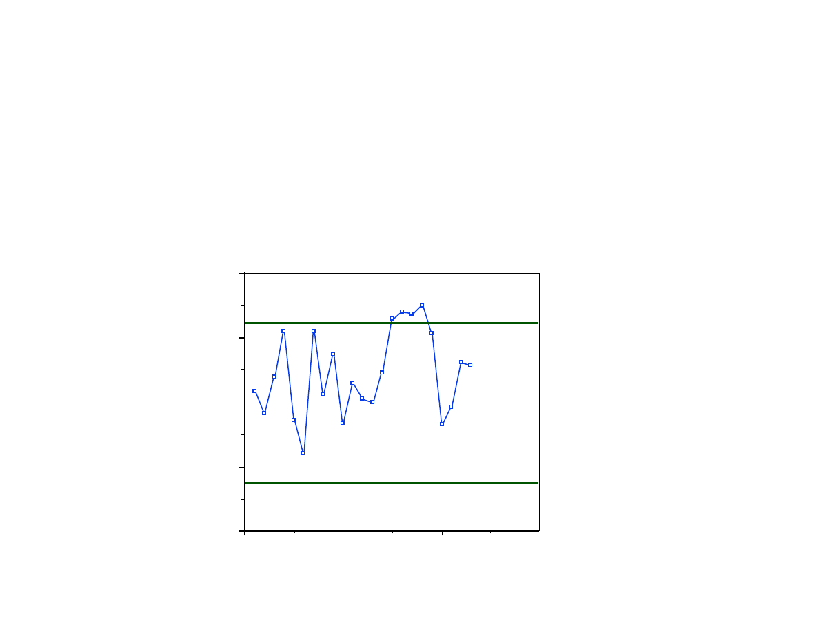
Group points and use the average in order to plot a known

(normal) statistic.
Assume that the first 10 groups of 4 are in Statistical

Control. Limits are set for type I error at 0.05.

30

20

10

0

-2

-1

0

1

2

LCL -1.2

UCL 1.2

Lecture 10: Introduction to Statistical Process Control

Spanos

EE290H F05

7

Example (cont.)

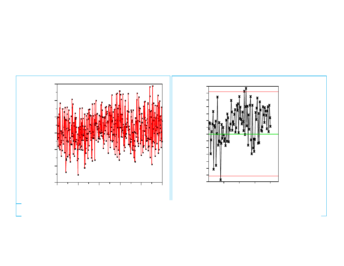
• The idea is that the average is normally distributed.
• Its standard deviation is estimated at .6333 from the first

10 groups.

• The true mean (

μ) is assumed to be 0.00 (furnace

temperature in control).

• There is only 5% chance that the average will plot

outside the

μ+/- 1.96 σ limits if the process is in control.

In general:
UCL =

μ + k σ

LCL =

μ - k σ

where

μ and σ relate to the statistic we plot.

Lecture 10: Introduction to Statistical Process Control

Spanos

EE290H F05

8

Another Example

Plot

small shift

0.850

0.900

0.950

1.000

1.050

1.100

1.150

0

100

200

300

400

500

small shift

Variable Control Charts

Mean of small shift

0.930

0.950

0.970

0.990

1.010

1.030

1.050

1.070

25

50

75

100

µ0=1.0006

LCL=0.9387

UCL=1.0626

Mean of small shift

Original data

Averaged Data (n=5)

Lecture 10: Introduction to Statistical Process Control

Spanos

EE290H F05

9

How the Grouping Helps

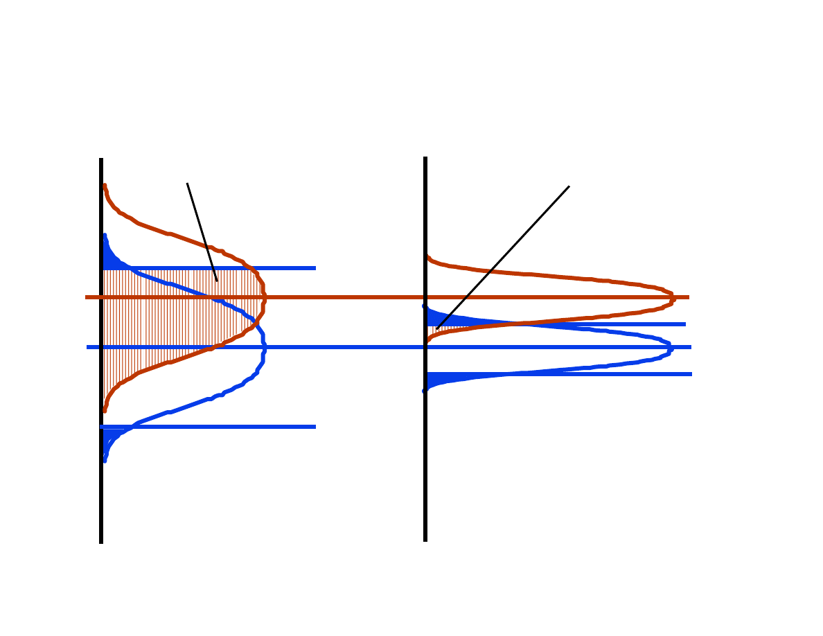
Small Group Size,

large

β.

Large Group Size,

smaller

β for same α.

Bad

Good

Lecture 10: Introduction to Statistical Process Control

Spanos

EE290H F05

10

Average Run Length

• If the type I error (

α) depends on the original (proper)

parameter distribution and the control limits, ...

• ... the type II error (

β) depends on the position of the

shifted (faulty) distribution with respect to the control
limits.

• The average run length (ARL) of the chart is defined as

the average number of samples between alarms.

• ARL, in general, is 1/

α when the process is good and

1/(1-

β) when the process is bad.

Lecture 10: Introduction to Statistical Process Control

Spanos

EE290H F05

11

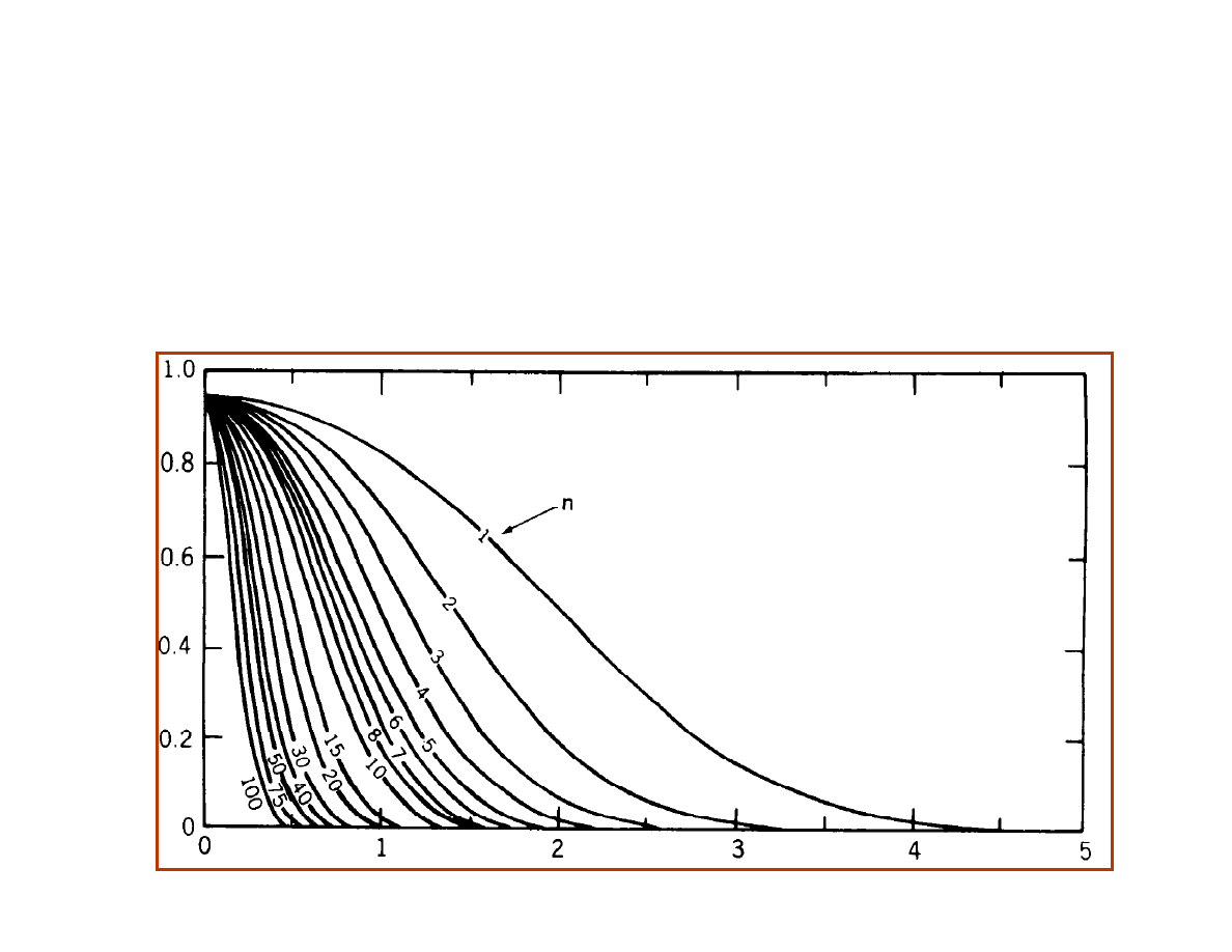
The Operating Characteristic Curve

Fig. 4-5 from Montgomery, pp. 110

These curves are drawn
for

α = 0.05

β

deviation in

#σ

The Operating Characteristic of the chart shows the

probability of missing an alarm vs. the actual process shift.
Its shape depends on the statistic, the subgroup size and

the control limits.

Lecture 10: Introduction to Statistical Process Control

Spanos

EE290H F05

12

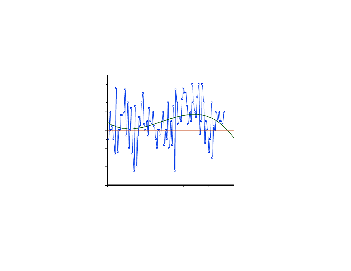
Pattern Analysis

Other rules exist: Western Electric, curve fitting,

Fourier analysis, pattern recognition...

100

80

60

40

20

0

-3

-2

-1

0

1

2

3

Lecture 10: Introduction to Statistical Process Control

Spanos

EE290H F05

13

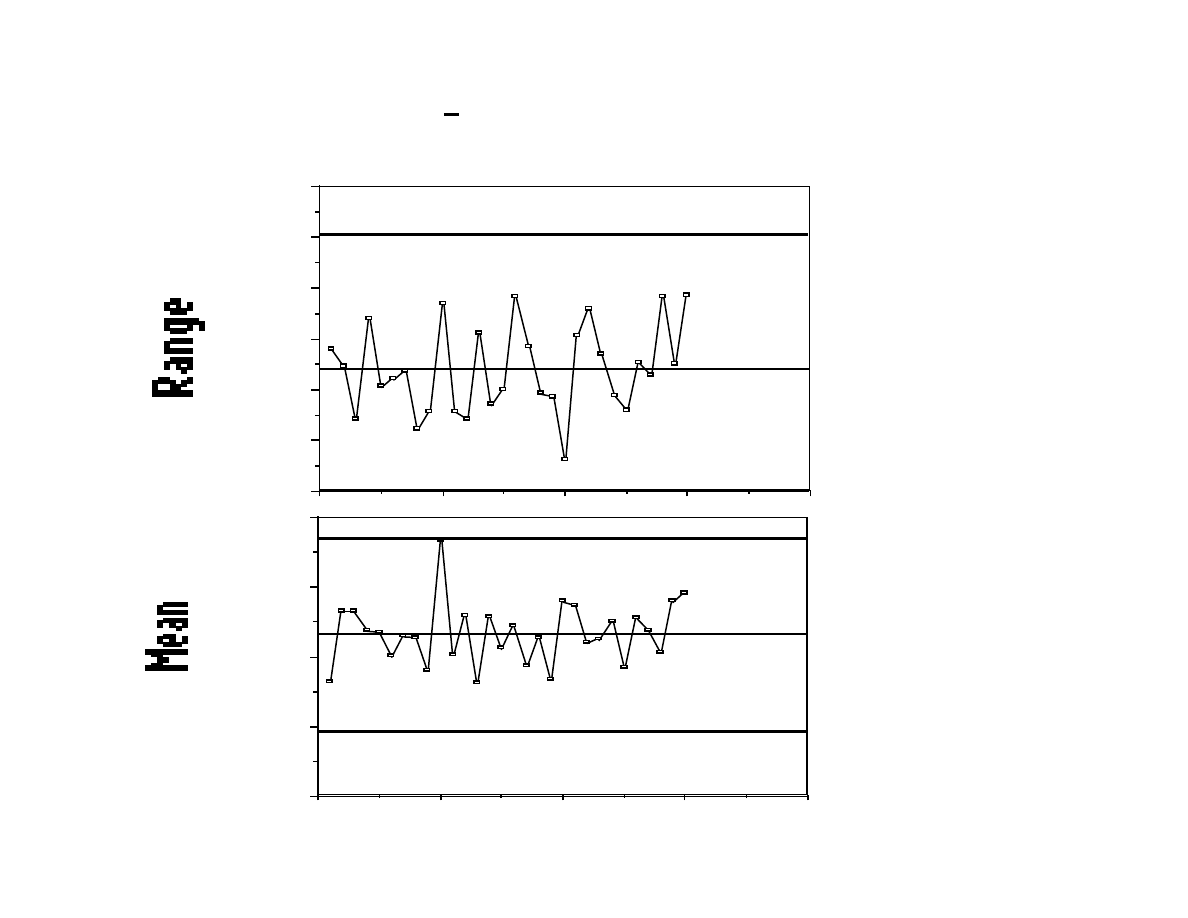
Example: Photoresist Coating

• During each shift, five wafers are coated with photoresist

and soft-baked. Resist thickness is measured at the
center of each wafer. Is the process in control?

• Questions that can be asked:

a) Is group variance "in control"?
b) Is group average "in control"?
c) Is there any difference between shifts A and B?

• In general, we can group data in many different ways.

Lecture 10: Introduction to Statistical Process Control

Spanos

EE290H F05

14

Range and x chart for all wafer groups.

0

100

200

300

400

500

600

LCL 0.0

UCL 507.09

40

30

20

10

0

7600

7700

7800

7900

8000

Wafer Groups

LCL 7694.52

UCL 7971.32

Lecture 10: Introduction to Statistical Process Control

Spanos

EE290H F05

15

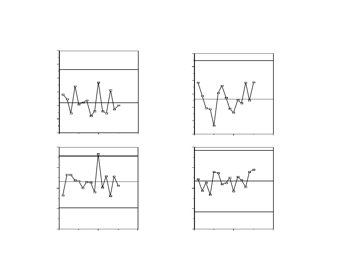
Comparing runs A and B

20

10

0

0

100

200

300

400

500

600

Range, Shift B

260

550

20

10

0

0

100

200

300

400

500

600

Range, Shift A

220

465

20

10

0

7600

7700

7800

7900

8000

Mean, Shift A

7704

7831

7958

20

10

0

7600

7700

7800

7900

8000

Mean, Shift B

7685

7835

7985

Lecture 10: Introduction to Statistical Process Control

Spanos

EE290H F05

16

Why Use a Control Chart?

• Reduce scrap and re-work by the systematic

elimination of assignable causes.

• Prevent unnecessary adjustments.
• Provide diagnostic information from the shape of

the non random patterns.

• Find out what the process can do.
• Provide immediate visual feedback.
• Decide whether a process is production worthy.

Lecture 10: Introduction to Statistical Process Control

Spanos

EE290H F05

17

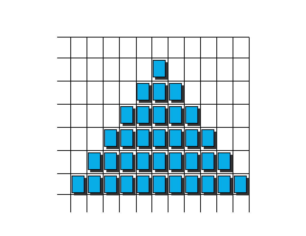
The Control Chart for Controlling Dice Production

Lecture 10: Introduction to Statistical Process Control

Spanos

EE290H F05

18

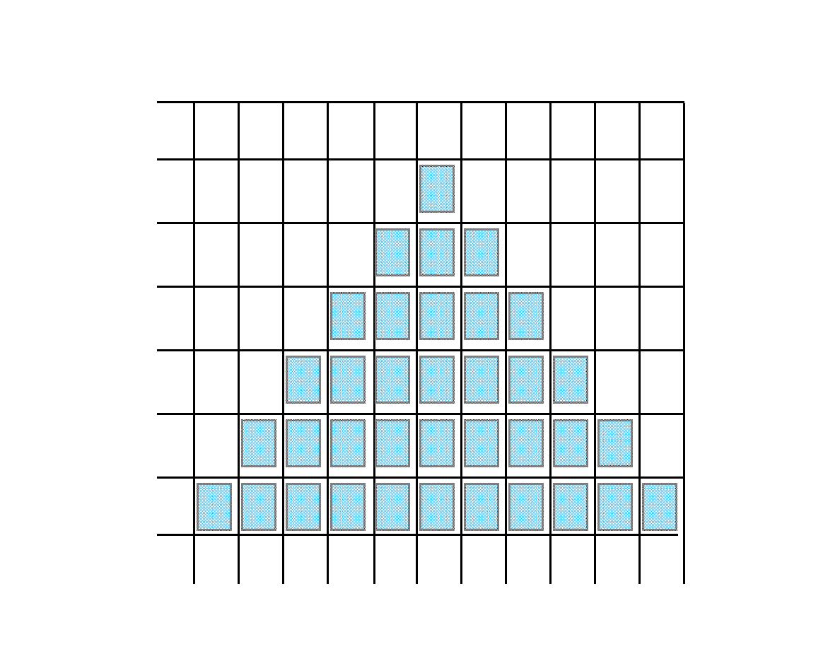
The Reference Distribution

2

3

4

5

6

7

8

9 10 11 12

1

2

3

4

5

6

7

Lecture 10: Introduction to Statistical Process Control

Spanos

EE290H F05

19

The Actual Histogram

2

3

4

5

6

7

8

9 10 11 12

1

2

3

4

5

6

7

Lecture 10: Introduction to Statistical Process Control

Spanos

EE290H F05

20

In Summary

• To apply SPC we need:
• Something to measure, that relates to

product/process quality.

• Samples from a baseline operation.
• A statistical “model” of the variation of the

process/product.

• Some physical understanding of what the

process/product is doing.