Matlab Image Processing Toolbox - introduction

Computer Image processing

Institute of Computer Modelling

Cracow University of Technology

At the beginning...
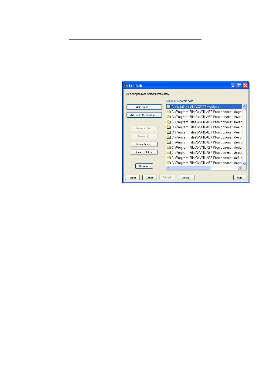
Set files path:

Paths are defined in the window Path
Browser (File/Set Path) and are stored
in the file called pathdef.m.

Variables, vectors and matrices definition

In Matlab a matrix is the main form of variables representation. This embraces one-
dimensional matrices (vectors), multi-dimensional matrices, and scalar variables, represented
by 1x1 matrices, as well.

Example 1
>> x = 22
x =
22
>> whos
Name Size Bytes Class
x 1x1 8 double array
Grand total is 1 element using 8 bytes
>>
X variable represented by 1x1 matrix.

Example 2: horizontal vector
>> y = [1 2 3 4]
y =
1 2 3 4
>> whos y
Name Size Bytes Class
y 1x4 32 double array
Grand total is 4 elements using 32 bytes

Example 3: vertical vector
>> y = [1 ; 2 ; 3 ; 4]
y =
1
2
3
4
>> whos y
Name Size Bytes Class
y 4x1 32 double array
Grand total is 4 elements using 32 bytes

We can achieve the same result using transposition (in Matlab we use apostrophe)
>> z = [1 2 3 4]
z =
1 2 3 4
>> z = z'
z =
1
2
3
4

Or:
>> z2 = [1 2 3 4]'
z2 =
1
2
3
4

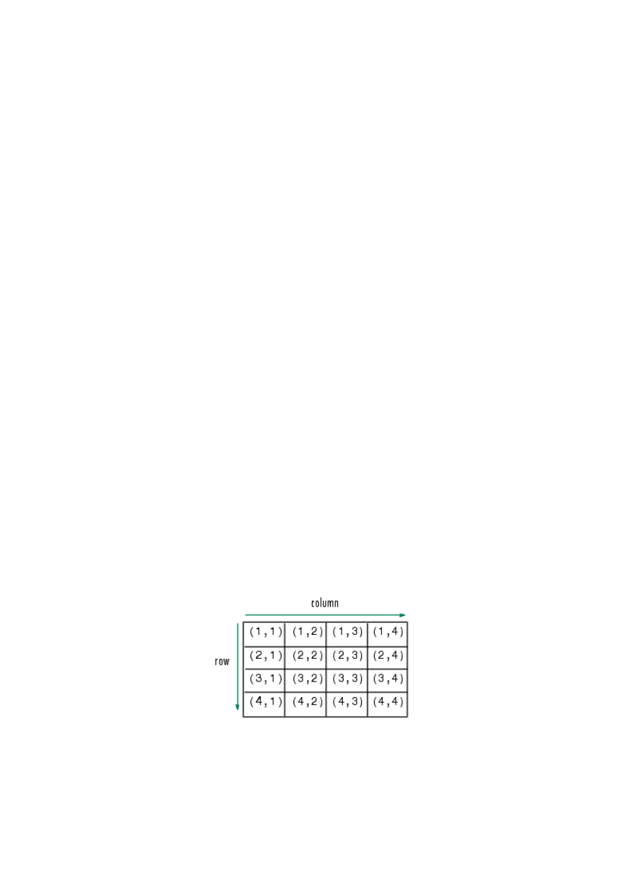
Two-dimensional matrices creation

Example 4: empty matrix
>> m = []
m =
[]

Example: matrix 3x4
>> m = [1 2 3 4 ; 5 6 7 8 ; 9 10 11 12]
m =
1 2 3 4
5 6 7 8
9 10 11 12

Individual rows separated by semicolon.
Very often functions that help to create specific matrices types are useful.

eye(... , ...) creates the matrix with ones at the diagonal:

>> eye(3,3)
ans =
1 0 0
0 1 0
0 0 1

Another similar functions:

>> ones(2,3)
ans =
1 1 1
1 1 1
>> zeros(3,2)
ans =
0 0
0 0
0 0
>> rand(2,2)
ans =
0.9501 0.6068
0.2311 0.4860
>> randn(2,2)
ans =
-0.4326 0.1253
-1.6656 0.2877
rand(...) returns a matrix with pseudorandom values in a uniform distribution, and randn(...) –
in a normal distribution.

The variable ans always stores the result of the last operation. When you don’t specify the
output argument, Matlab creates the variable ans automatically. The reference to the single
matrix elements is made by using indexes:

>> x = rand(2,3)
x =
0.8913 0.4565 0.8214
0.7621 0.0185 0.4447
>> x(1, 2)
ans =
0.4565

Warning: Indexation starts from 1, not from 0!

Indexes assignment:

>> x(1, 2) = 222
x =
0.8913 222.0000 0.8214
0.7621 0.0185 0.4447

We can use ranges, when the matrices are created, and when we want to refer to their
elements, as well.

Example 5: vector with the elements from 1 to 10
>> v = 1:10
v =
1 2 3 4 5 6 7 8 9 10

Example 6: vector with the elements from 1 to 10 with 0.8 step
>> v = 1:0.8:10
v =
1.0000 1.8000 2.6000 3.4000 4.2000 5.0000 5.8000 6.6000 7.4000 8.2000 9.0000 9.8000

The similar for the matrix::
>> m = [ 1:2:10 ; 2:0.5:4]
m =
1.0000 3.0000 5.0000 7.0000 9.0000
2.0000 2.5000 3.0000 3.5000 4.0000

If we want to take, for example, the second column or the third row from the matrix, we can
write:
>> x = rand(3,4)
x =
0.6154 0.7382 0.9355 0.8936
0.7919 0.1763 0.9169 0.0579
0.9218 0.4057 0.4103 0.3529
>> y = x(:,2)
y =
0.7382
0.1763
0.4057
>> z = x(3,:)
z =
0.9218 0.4057 0.4103 0.3529

Or an example of the more complicated matrix “cutting”, for example rows from 2 to 4,
columns from 3 to 5:
>> x = rand(5,6)
x =
0.8132 0.6038 0.4451 0.5252 0.6813 0.4289
0.0099 0.2722 0.9318 0.2026 0.3795 0.3046
0.1389 0.1988 0.4660 0.6721 0.8318 0.1897
0.2028 0.0153 0.4186 0.8381 0.5028 0.1934
0.1987 0.7468 0.8462 0.0196 0.7095 0.6822
>> y = x(2:4,3:5)
y =
0.9318 0.2026 0.3795
0.4660 0.6721 0.8318
0.4186 0.8381 0.5028

In a similar way we can execute the substitution:

>> x = rand(2,3)
x =
0.3028 0.1509 0.3784
0.5417 0.6979 0.8600
>> y = [ 22 22 22 ]
y =
22 22 22
>> x(1,:) = y
x =
22.0000 22.0000 22.0000
0.5417 0.6979 0.8600

We can also remove, for example the second row of the given matrix in this way:

>> x = rand(3,4)
x =
0.1365 0.1991 0.2844 0.9883
0.0118 0.2987 0.4692 0.5828
0.8939 0.6614 0.0648 0.4235
>> x(2,:) = []
x =
0.1365 0.1991 0.2844 0.9883
0.8939 0.6614 0.0648 0.4235

What will happen if we assign the matrix x to the variable y, and then we change values in the
y matrix? Will this change be visible in x? If the operation x=y creates “a deep copy” or of x,
or copies only the references to x?

>> x = zeros(3)
x =
0 0 0
0 0 0
0 0 0
>> y = x
y =
0 0 0
0 0 0
0 0 0
>> y(1,1) = 22
y =
22 0 0
0 0 0
0 0 0
>> x
x =
0 0 0
0 0 0
0 0 0

Operations on matrices

Two matrices can be multiplied only when they have the same dimensions, i.e. when the
m=number of columns in the first one equals the number of rows in the second one.

Example 7:
>> x = rand(3,2)
x =
0.8537 0.8998
0.5936 0.8216
0.4966 0.6449
>> y = rand(2,4)
y =
0.8180 0.3420 0.3412 0.7271
0.6602 0.2897 0.5341 0.3093
>> z = x * y
z =
1.2923 0.5526 0.7718 0.8990
1.0280 0.4410 0.6413 0.6857
0.8320 0.3567 0.5139 0.5605
Natomiast:
>> x = rand(3,2)
x =
0.8385 0.7027
0.5681 0.5466
0.3704 0.4449
>> y = rand(3,4)
y =
0.6946 0.9568 0.1730 0.2523
0.6213 0.5226 0.9797 0.8757
0.7948 0.8801 0.2714 0.7373
>> z = x * y
??? Error using ==> *
Inner matrix dimensions must agree.

1x1 matrix that represents the scalar vector is an exception:

>> a = 22
a =
22
>> x = ones(3)
x =
1 1 1
1 1 1
1 1 1
>> x = a*x
x =
22 22 22
22 22 22
22 22 22

As we can see, every matrix element was multiplied by 22.
Apart from matrices operations, we can execute the table operations (element by element).
For this purpose, we use . (dot) operator.

An example of multiplication:
>> x = 2 * ones(2)
x =
2 2
2 2
>> y = 3 * ones(2)
y =
3 3
3 3
>> z = x * y
z =
12 12
12 12
>> z = x .* y
z =
6 6
6 6

Another example – we want to raise the every matrix element to the third power:
>> x = 2 * ones(2)
x =
2 2
2 2
>> x = x .^ 3
x =
8 8
8 8

While, when we raise the whole matrix to the third power, we obtain:
>> x = 2 * ones(2)
x =
2 2
2 2
>> x = x^3
x =
32 32
32 32

The other operations on matrices:

A(:,end) – printing the last column
A(end,:) – printing the last row
size(A) – the size of a matrix
>> x = rand(3,4)
x =
0.9901 0.4983 0.3200 0.4120
0.7889 0.2140 0.9601 0.7446

0.4387 0.6435 0.7266 0.2679
>> size(x)
ans =
3 4
>> [rows, columns] = size(x)
rows =
3
columns =
4

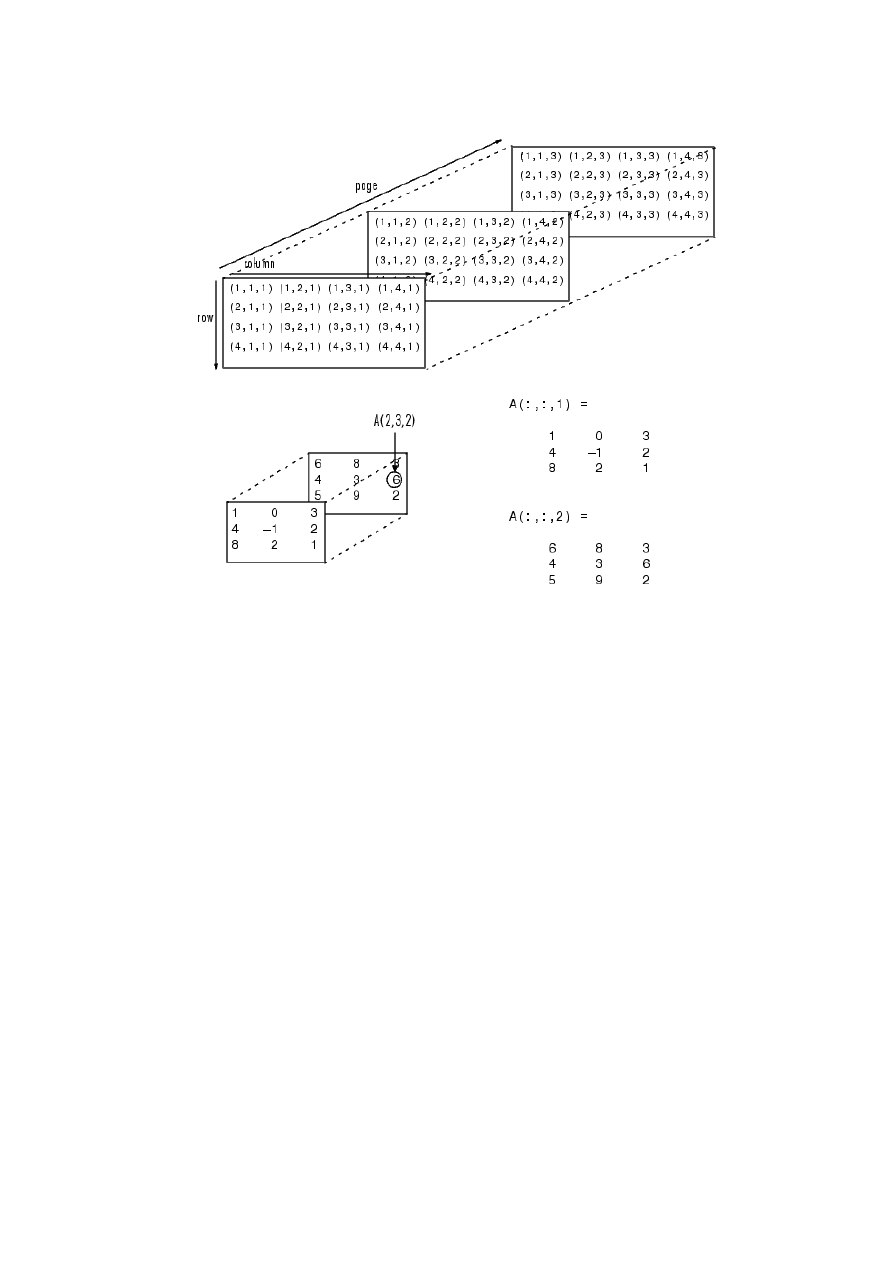
Multi-dimensional matrices

We can work with the matrices that have more than 2 dimensions:

>> x = ones(2,3, 2)
x(:,:,1) =
1 1 1
1 1 1
x(:,:,2) =
1 1 1
1 1 1
>> x(:,:,2) = x(:,:,2) * 22
x(:,:,1) =
1 1 1
1 1 1
x(:,:,2) =
22 22 22
22 22 22
>> x(2,1,1) = 333
x(:,:,1) =
1 1 1
333 1 1
x(:,:,2) =
22 22 22
22 22 22

Arithmetical operations

Multiplication
C=A+B
Subtraction
Analogous...
Table multiplication „*”
C = A * B matrix multiplication (the sum of products of the i row of the matrix A and k
column of the matrix B)
C=A.*B table operation (multiplications between elements with the same index)
Division
Analogous
In a table calculation:
C=A./B
Expotentiation
C=A.^2 to raise to the second power
Root extraction
C=sqrt(A)
Transposition
„’ ”
Matrix transposition A.’
Inversion
„inv”
Inverted matrix
C=inv(B)

Logical operators

< A<B less than
<= A<=B less or equal than
> A>B more than
>= A>=B more or equal than
== A==B equal
~= A~=B different
& and(A,B) AND – logical product
| or(A,B) OR – logical sum
~ not(A) NOT - negation
Xor xor(A,B) EXCLUSIVE OR – strong disjunction

Example 8:
>> x = rand(2,3)
x =
0.0164 0.5869 0.3676
0.1901 0.0576 0.6315
>> y = rand(2,3)
y =
0.7176 0.0841 0.4418
0.6927 0.4544 0.3533
>> x < y
ans =
1 0 1
1 1 0

Ones indicate elements, for which the condition has TRUE value.

The other operations:

any(A) – returns 1, if any of the column elements is non-zero
all(A) - returns 1, if all of the column elements are non-zero
find – finds the elements that fulfill the condition
„all” and „any” work on matrix columns, or in the case of multi-dimensional matrix, on the
first non-single-element dimension

Example 9: to reset the elements with the values more than 0.5 in x:
x =
0.1536 0.6992 0.4784
0.6756 0.7275 0.5548
>> indx = find( x > 0.5 )
indx =
2
3
4
6
>> x(indx) = 0
x =
0.1536 0 0.4784
0 0 0

Or shorter:
x =
0.1210 0.7159 0.2731
0.4508 0.8928 0.2548
>> x( find(x>0.5) ) = 0
x =
0.1210 0 0.2731
0.4508 0 0.2548

Exercise: For two matrices with the same dimensions reset the elements at the positions in
which they are different.

Exercise: Examine the following functions:
Roundings
Create a vector x = [2.2, -3.6; -4.7, 8.1]
ceil (x) % to the higher value
ans =
3 -3
-4 9
fix(x) % elimination of the fractional part
ans =
2 -3
-4 8
floor(x) % to the lower value
ans =
2 -4
-5 8
round(x) % to the nearest integer
ans =
2 -4
-5 8
abs(x) % absolute value
ans =
2.2000 3.6000
4.7000 8.1000

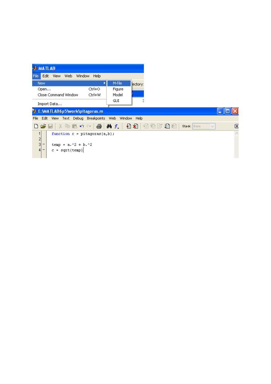
Script construction (M-file)
The file containing the Matlab script (m-file) is a text file with .m extention.
It can contain sequences of Matlab commands or evoke the other m-files.
It can activate itself.

There are two file types: scripts and functions.
Scripts contain commands sequences and they work using variables that are accessible in the
workspace. They are used for data entering and storage, repeating sequences simplification,
algorithms.
Functions – functions algorithms working on local or global variables. They communicate
through the global variables (defined by the command “global”) or/and formal parameters.
They have to begin with „function”.
function[list of output arguments]= function_name (list of input arguments)

Input and output arguments are local. A bracket [] can be skipped if we have one or zero
arguments.

Example 10:
Create the new file pitagoras.m

The function pitagoras returns the value c. Notice that a, b and c can be matrices.
>> x = pitagoras(3,4)
temp =
25
c =
5
x =
5

For matrices we also obtain the correct result:
>> a = [1 2; 3 4]
a =
1 2
3 4
>> b = [2 3; 4 5]
b =
2 3
4 5
>> x = pitagoras(a,b)
temp =
5 13
25 41
c =
2.2361 3.6056
5.0000 6.4031
x =
2.2361 3.6056
5.0000 6.4031

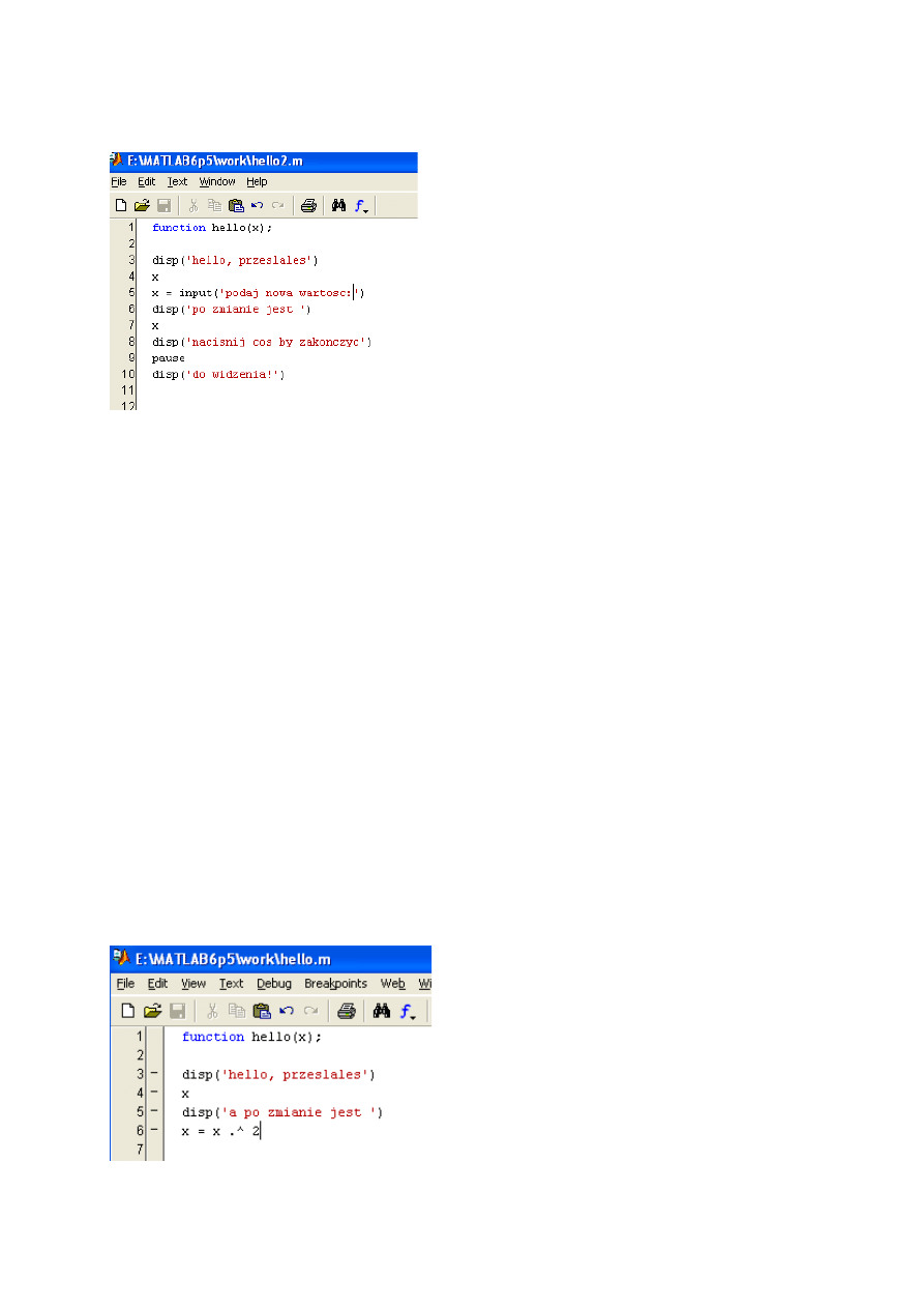
The example of a function, which shows how print a text and get the data from the keyboard.

>> hello(3)
hello, przeslales 3.00000 0
podaj nowa wartosc:22
x =
22
nacisnij cos by zakonczyc...
do widzenia!

Exercise: Check what will happen after writing
>> x = 33
x =
33
>> hello(x)
hello, przeslales 33.000000
podaj nowa wartosc:22
x =
22
nacisnij cos by zakonczyc...
do widzenia!
>> x

What wil the value of x? Whether the change has changed the global or local value? What the
situation is, if the function has received the matrix? Whether it makes the deep copy of the
matrix?

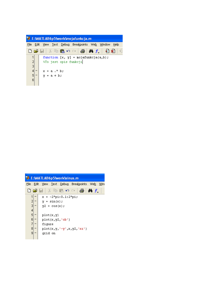
This is the function that returns two values. The semicolon after the line means that the result
is not printed.

>> a = 3*ones(2)
a =
3 3
3 3
>> b = 2*ones(2)
b =
2 2
2 2
>> [xx yy] = mojafunkcja(a,b)
xx =
6 6
6 6
yy =
5 5
5 5
Help using:
>> help mojafunkcja
To jest opis funkcji

And a short script that doesn’t define any functions, but allows writing and executing the
several functions. In this case, we will draw the sine and cosine function.
Calling:
>> sinus

Global variables (accessible everywhere – even in functions) are defined with a shell global.

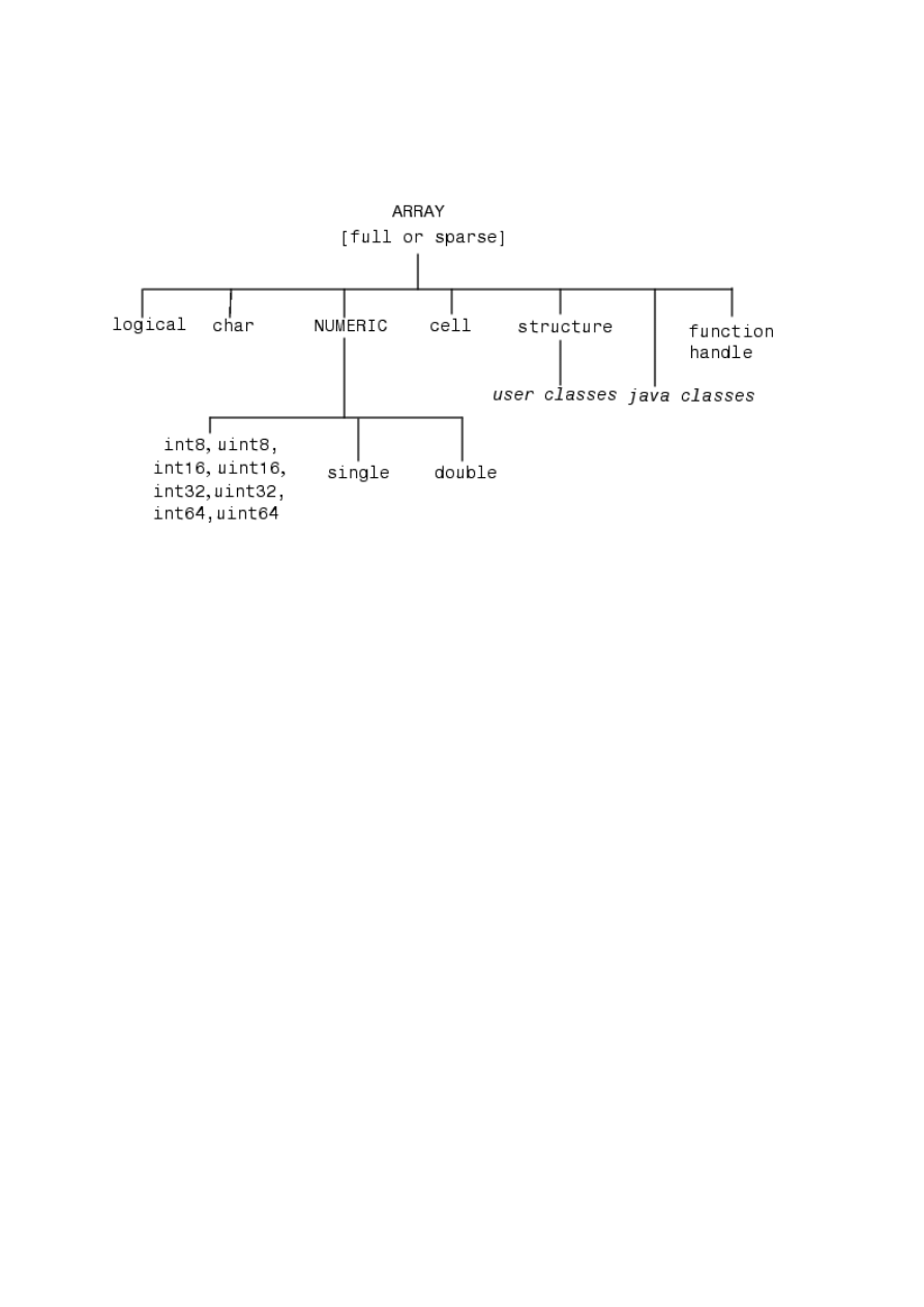
Variables types in Matlab

Programming

Keywords
>> iskeyword
ans =
'break'
'case'
'catch'
'continue'
'else'
'elseif'
'end'
'for'
'function'
'global'
'if'
'otherwise'
'persistent'
'return'
'switch'
'try'
'while'

if, else, elseif
if logical_expression
statements
end
E.g.:

if n < 0 % If n negative, display error message.
disp('Input must be positive');
elseif rem(n,2) == 0 % If n positive and even, divide by 2.

A = n/2;
else
A = (n+1)/2; % If n positive and odd, increment and divide.
End

switch
switch expression (scalar or string)
case value1
statements % Executes if expression is value1
case value2
statements % Executes if expression is value2
.
otherwise
statements % Executes if expression does not match any case
end
E.g.:

switch input_num
case -1
disp('negative one');
case 0
disp('zero');
case 1
disp('positive one');
otherwise
disp('other value');
end

while
while expression
statements
end
Np.
n = 1;
while prod(1:n) < 1e100
n = n + 1;
end

for
for index = start:increment:end
statements
end
Np.

for i = 1:m
for j = 1:n
A(i,j) = 1/(i + j - 1);
end
end

continue
e.g.:

fid = fopen('magic.m','r');
count = 0;
while ~feof(fid)
line = fgetl(fid);
if isempty(line) | strncmp(line,'%',1)
continue
end
count = count + 1;
end
disp(sprintf('%d lines',count));

break
e.g.:

fid = fopen('fft.m','r');
s = '';
while ~feof(fid)
line = fgetl(fid);
if isempty(line)
break
end
s = strvcat(s,line);
end
disp(s)

Simple examples from image processing

Write help imread to check what types of files can be used in Matlab Image Processing
Toolbox.

Example: m-plik simple_image_proc.m
imfinfo('portret.jpg')
disp('dalej...'); pause
im = imread('portret.jpg');
imshow(im)
disp('dalej...'); pause
disp('zmiana mapy kolorow na hsv');
colormap(hsv)
disp('dalej...'); pause
disp('zmiana mapy kolorow na jet');
colormap(jet)
disp('dalej...'); pause
disp('zmiana mapy kolorow na losowa o 2 barwach');
colormap( rand(2,3) )
disp('dalej...'); pause
disp('zmiana mapy kolorow na losowa o 4 barwach');
colormap( rand(4,3) )
disp('dalej...'); pause
disp('zmiana mapy kolorow na losowa o 8 barwach');

colormap( rand(8,3) )
disp('dalej...'); pause
disp('zmiana mapy kolorow na losowa o 12 barwach');
colormap( rand(12,3) )
disp('dalej...'); pause
disp('koniec...');

Example 12: m-plik simple_image_proc2.m
imfinfo('e0102.bmp')
disp('dalej...'); pause
im = imread('e0102.bmp');
imshow(im)
disp('dalej...'); pause
disp('tylko skladowa czerwona jako czarno-biala')
imshow(im(:,:,1))
disp('dalej...'); pause
disp('tylko skladowa zielona jako czarno-biala')
imshow(im(:,:,2))
disp('dalej...'); pause
disp('tylko skladowa niebieska jako czarno-biala')
imshow(im(:,:,3))
disp('dalej...'); pause
disp('tylko skladowa czerwona z mapa kolorow')
imshow(im(:,:,1))
map = zeros(256, 3)
map(:,1) = [0:(1/255):1]'
colormap(map)
disp('dalej...'); pause
disp('tylko skladowa zielona z mapa kolorow')
imshow(im(:,:,2))
map = zeros(256, 3)
map(:,2) = [0:(1/255):1]'
colormap(map)
disp('dalej...'); pause
disp('tylko skladowa niebieska z mapa kolorow')
imshow(im(:,:,3))
map = zeros(256, 3)
map(:,3) = [0:(1/255):1]'
colormap(map)
disp('dalej...'); pause
disp('koniec');

Type of image checking

isbw(A) – checks, if the image is binary
isgray(A) – checks, if the image is in the grayscale
isind(A) – checks, if the image is in the indexed colour
isrgb(A) – checks, if the image is in the RGB colour

The other information

Special signs
= value assignation
[ ] creation of empty matrices, function output arguments, matrices combining (value
declaration after the sign = )
{ } structure indexes and cell tables
( ) function input arguments, table indexes, brackets necessary to define the operation
sequences (never after =,<,>)
. dot operator, after integer, separator of objects names, change of operation from the matrix
into the table one,
… command continuation in the next line,
, command, indexes, function indexes separator,
; the end of the matrix raw, stopping the result printing,
% command, remark start,
: vector creation, matrix indexing,
‘ a chain (apostrophe before and at the end), matrix transposition operator,

Predefined constants

Inf (infinitive) – to the infinity ∞
1/0
log(0)
Notice:
Inf-Inf and Inf/Inf – give NaN (Not-a-Number) as the result

NaN (Not-a-Number)
The result of every NaN operation, e.g. sqrt(NaN)
(+Inf)+(-Inf)
0*Inf
0/0 oraz Inf/Inf
Notice:
Two NaN numbers are not equal, so logical operations on NaN give always 0 (false), with
exception of ~=
(different, non equal )
NaN ~= NaN
ans =
1
NaN == NaN
ans =
0
NaN-s in a vector are treated as different (non repetitive) elements
unique([1 1 NaN NaN]) % find unique elements of vector

ans =
1 NaN NaN
isnan([1 1 NaN NaN]) % isnan serves to find NaN in a matrix, returns 1, if there is
NaN anywhere
ans =
0 0 1 1