1

DSaA 2012/2013

String matching

Data Structures and Algorithms

2

DSaA 2012/2013

String matching

String matching algorithms:
• Naive
• Rabin-Karp
• Finite automaton
• Knuth-Morris-Pratt (KMP)

ε – epsilon, δ – delta, φ – phi, σ – sigma, π - pi

3

DSaA 2012/2013

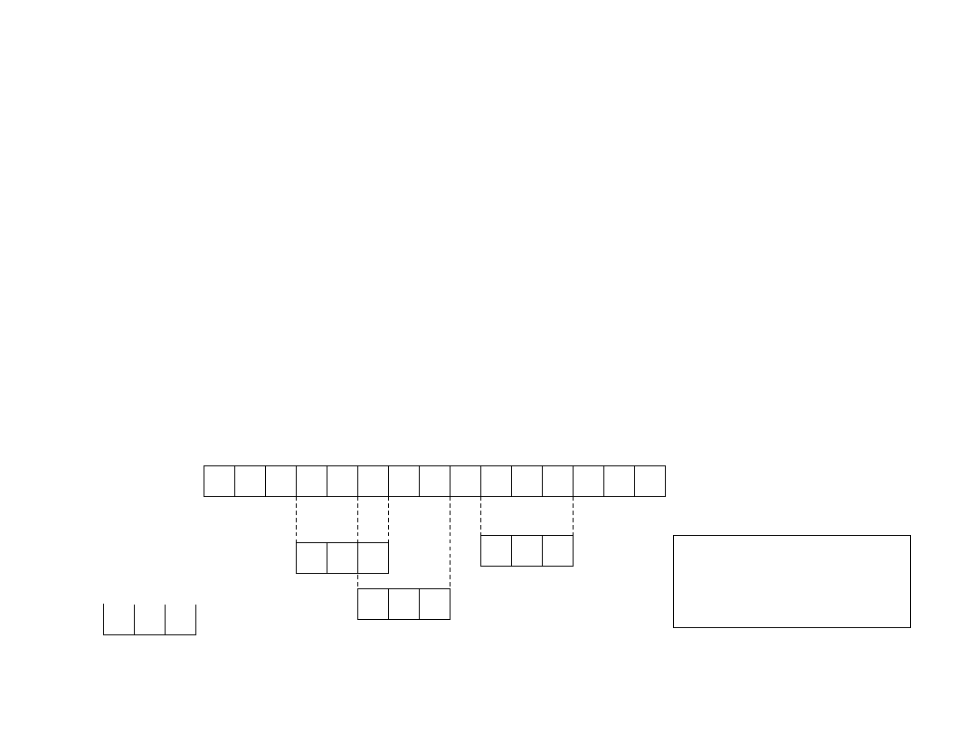
String matching problem

•

We assume that the text is an array T [1..n] of length n and that the pattern
is an array P[1..m] of length m

≤ n. We further assume that the elements of

P and T are characters drawn from a finite alphabet

S

. For example, we

may have

S

= {0, 1} or

S

= {a, b,. . . , z}. The character arrays P and T are

often called strings of characters.

•

We say that pattern P occurs with shift s in text T (or, equivalently, that
pattern P occurs beginning at position s + 1 in text T) if 0

≤ s ≤ n - m and

T [s + 1..s + m] = P[1..m] (that is, if T [s + j] = P[ j], for 1

≤ j ≤ m). If P occurs

with shift s in T , then we call s a valid shift; otherwise, we call s an invalid
shift. The string-matching problem is the problem of finding all valid shifts
with which a given pattern P occurs in a given text T

Text T

Pattern P

b a b a

a c b a

a a b a

a b a

b b a

a b a

a b a

a b a

3 occurrences
of pattern with shifts
3, 5, 9

15

1

2

3

4

5

6

7

8

9 10 11 12 13 14

1

2

3

4

DSaA 2012/2013

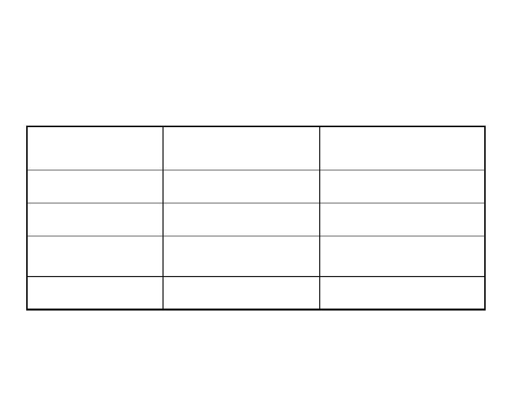
Complexity - comparison

Algorithm

Preprocessing time

Worse case

Matching time

Naive

0

O((n-m+1)m)

Rabin-Karp



(m)

O((n-m+1)m)

Finite automaton

O(m|

S

|)



(n)

Knutt-Morris-Pratt



(m)



(n)

5

DSaA 2012/2013

Notation and terminology

• We shall let

S

* (read "sigma-star") denote the set of all

finite-length strings formed using characters from the

alphabet

S

. In this lecture, we consider only finite-length

strings. The zero-length empty string, denoted

e

, also

belongs to

S

*. The length of a string x is denoted |x|. The

concatenation of two strings x and y, denoted xy, has

length |x| + |y| and consists of the characters from x

followed by the characters from y.

• We say that a string w is a prefix of a string x, denoted w

⊏ x, if x = wy for some string y



S

*. Note that if w

⊏ x,

then |w|

≤ |x|. Similarly, we say that a string w is a suffix

of a string x, denoted w

⊐ x, if x = yw for some y



S

*. It

follows from w

⊐ x that |w| ≤ |x|. The empty string

e

is

both a suffix and a prefix of every string. For example,

we have ab

⊏ abcca and cca ⊐ abcca. It is useful to note

that for any strings x and y and any character a, we have

x

⊐y if and only if xa⊐ya. Also note that ⊏ and ⊐ are

transitive relations.

6

DSaA 2012/2013

Notation and terminology

• Overlapping-suffix lemma:
Suppose that x, y, and z are strings such

that x

⊐z and y⊐z. If |x| ≤ |y|, then x⊐y. If

|x|

≥|y|, then y⊐x. If |x| = |y|, then x = y.

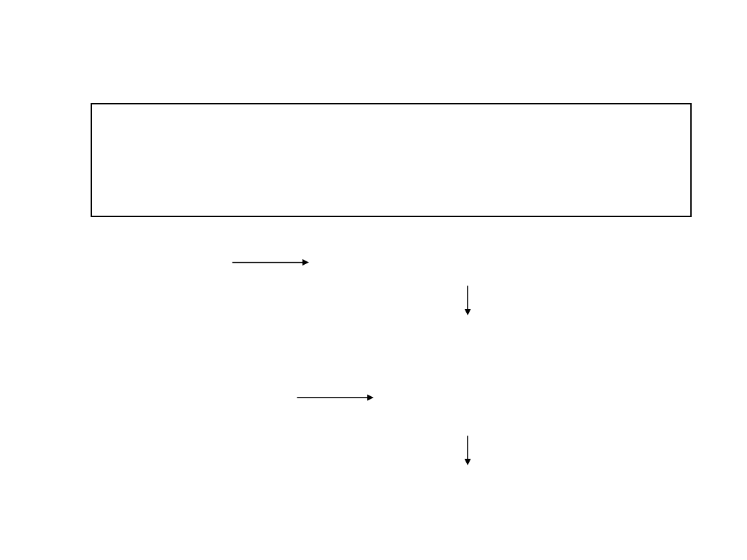
For brevity of notation, we shall denote the k-character prefix P[1..k]
of the pattern P[1..m] by P

k

. Thus, P

0

=

e

and P

m

= P = P[1..m]. Similarly,

we denote the k-character prefix of the text T as T

k

. Using this notation,

we can state the string-matching problem as that of finding all shifts s in
the range 0

≤ s ≤ n-m such that P ⊐T

s+m

.

The test "x = y" is assumed to take time



(t + 1), where t is the length of the

longest string z such that z

⊏x and z⊏y.

7

DSaA 2012/2013

Naive algorithm - code

{ 1}
{ 2}
{ 3}
{ 4}
{ 5}

Naive_String_Matcher(T,P)
n := length[T]
m := length[P]
for s:=0 to n-m do
if P[1..m]=T[s+1..s+m] then
print „patter occurs with shift” s

T=a

n

, P=a

m

(n-m+1)m character comparisons

Worse-case complexity: O((n-m+1)m)

T=„random”, P=„random”

average ≤2(n-m+1)
character comparisons

Average complexity: O(n-m+1)

T=a

n

, P=a

m-1

b

8

DSaA 2012/2013

The Rabin-Karp algorithm - idea

•

For expository purposes, let us assume that

S

= {0, 1, 2, . . . , 9}, so that each

character is a decimal digit. (In the general case, we can assume that each character

is a digit in radix-d notation, where d = |

S

|.) We can then view a string of k

consecutive characters as representing a length-k decimal number. The character

string

„31415” thus corresponds to the decimal number 31,415.

•

Given a pattern P[1..m], we let p denote its corresponding decimal value. In a similar

manner, given a text T[1..n], we let t

s

denote the decimal value of the length-m

substring T[s + 1..s + m], for s = 0, 1, . . . , n-m. Certainly, t

s

= p if and only if

T[s+1..s+m] = P[1..m]; thus, s is a valid shift if and only if t

s

= p. If we could compute

p in time



(m) and all the t

s

values in a total of



(n - m + 1) time, then we could

determine all valid shifts s in time



(m) +



(n-m+1) =



(n) by comparing p with each

of the t

s

's. We can compute p in time



(m) using Horner's rule:

p = P[m] + 10 (P[m - 1] + 10(P[m -

2] + · · · + 10(P[2] + 10P[1]) )).

•

The value t

0

can be similarly computed from T[1..m] in time



(m). To compute the

remaining values t

1

, t

2

, . . . , t

n-m

in time



(n - m), it suffices to observe that t

s+1

can be

computed from t

s

in constant time, since





]

1

[

]

1

[

10

10

1

1

















m

s

T

s

T

t

t

m

s

s

T=..314152.., m=5, t

s

=31415

t

s+1

=10(31415-10000

*

3)+2=14152

Problem! : p and t

s

may be too large to work with conveniently.

9

DSaA 2012/2013

The Rabin-Karp algorithm

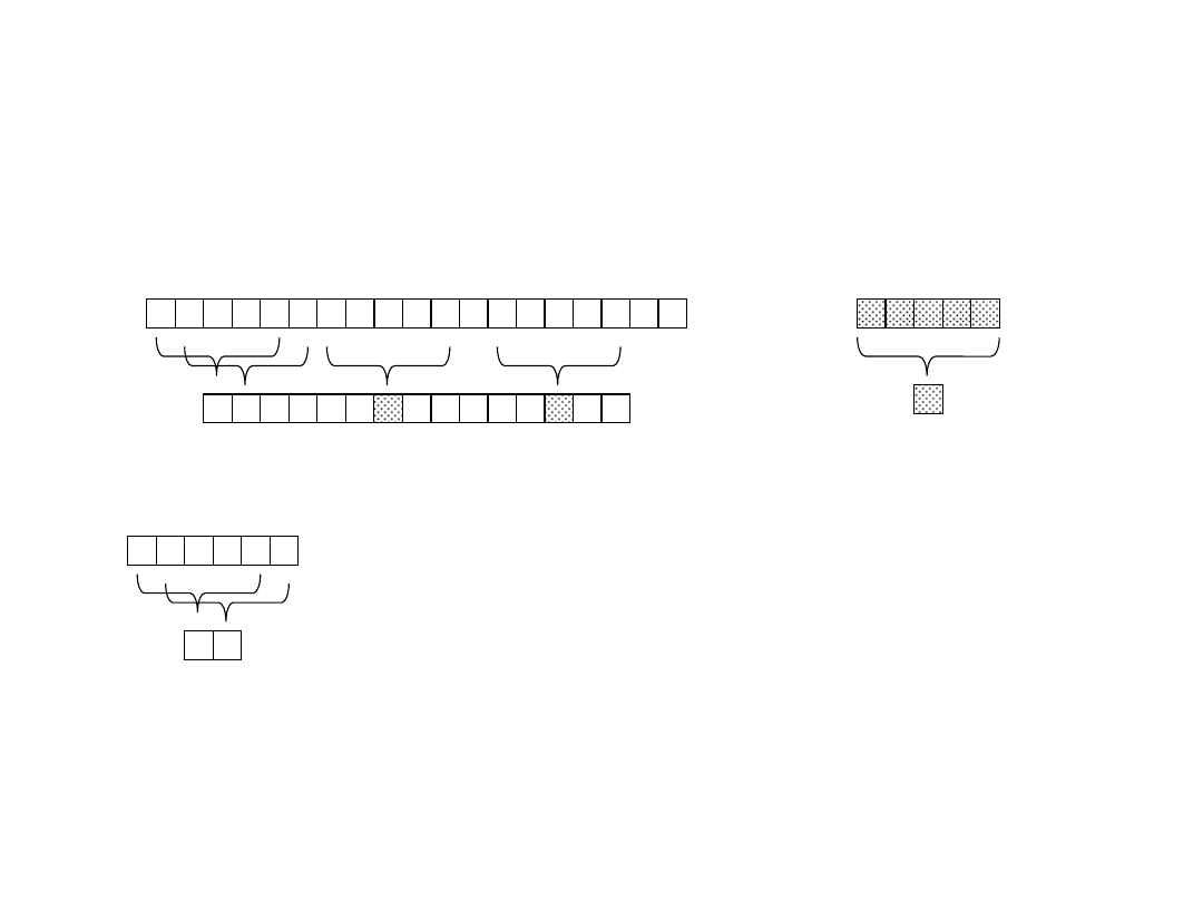
• We can compute p and the t

s

's modulo a

suitable modulus q.

2 3 5 9 0 2 3 1 4 1 5 2 6 7 3 9 9 2 1

3 1 4 1 5

7

8 9 3 11 0 1 7 8 4 5 10 11 7 9

…

…

11

q=13

valid
match

spurious
hit

2 3 5 9 0 2

8 9

35902 ≡ (23590 – 3*10000)*10+2 (mod 13)

≡ (8 – 2*3)*10 + 2 (mod 13)

≡ 9

 













q

m

s

T

h

s

T

t

d

t

s

s

mod

1

1

1















where





q

d

h

m

mod

1





10

DSaA 2012/2013

The Rabin-Karp algorithm - code

{ 1}
{ 2}
{ 3}
{ 4}
{ 5}
{ 6}
{ 7}
{ 8}
{ 9}
{10}
{11}
{12}
{13}
{14}

Rabin_Karp_Matcher(T,P)
n := length[T]
m := length[P]
h := d

m-1

mod q

p := 0
t

0

:= 0

for i:=1 to m do
p := (d*p+P[i]) mod q
t

o

:= (d*t

0

+T[i]) mod q

for s:=0 to n-m do
if p=t

s

then

if P[1..m]=T[s+1..s+m] then
print „patter occurs with shift” s
if s < n-m then
t

s+1

:=(d*(t

s

-T[s+1]*h)+T[s+m+1]) mod q

The modulus q is typically chosen as a prime such that dq just fits within
one computer word (double word)

11

DSaA 2012/2013

The Rabin-Karp algorithm - analysis

• RABIN-KARP-MATCHER takes



(m) preprocessing time, and its

matching time is



((n - m + 1)m) in the worst case, since (like the naive

string-matching algorithm) the Rabin-Karp algorithm explicitly verifies
every valid shift. If P = a

m

and T = a

n

, then the verifications take time



((n - m + 1)m), since each of the n - m + 1 possible shifts is valid.

• In many applications, we expect few valid shifts (perhaps some

constant c of them); in these applications, the expected matching time
of the algorithm is only O((n - m + 1) + cm) = O(n+m), plus the time
required to process spurious hits. After a heuristic analysis on an
assumption we can then expect that the number of spurious hits is
O(n/q), since the chance that an arbitrary t

s

will be equivalent to p,

modulo q, can be estimated as 1/q. Since there are O(n) positions at
which the test of line 10 fails and we spend O(m) time for each hit, the
expected matching time taken by the Rabin-Karp algorithm is

O(n) + O(m(v + n/q)),

where v is the number of valid shifts. This running time is O(n) if v=O(1)

and we choose q = m. That is, if the expected number of valid shifts is
small (O(1)) and the prime q is chosen to be larger than the length of
the pattern, then we can expect the Rabin-Karp procedure to use only
O(n + m) matching time. Since m



n, this expected matching time is

O(n).

12

DSaA 2012/2013

Finite automaton

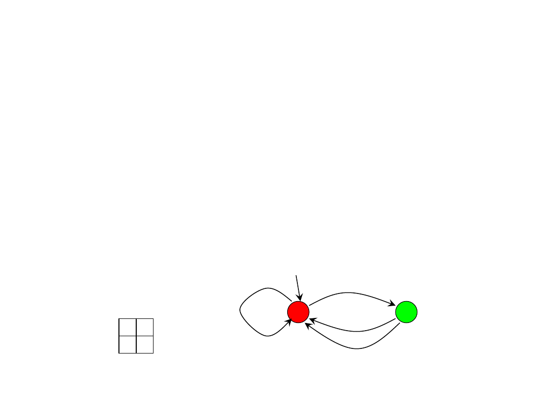
• A finite automaton M is a 5-tuple (Q, q

0

, A,

S

,

d

), where:

– Q is a finite set of states,
– q

0



Q is the start state,

– A



Q is a distinguished set of accepting states,

–

S

is a finite input alphabet,

–

d

is a function from Q

×

S

into Q, called the transition function of M.

The finite automaton begins in state q

0

and reads the characters of its

input string one at a time. If the automaton is in state q and reads

input character a, it moves ("makes a transition") from state q to

state

d

(q, a). Whenever its current state q is a member of A, the

machine M is said to have accepted the string read so far. An input

that is not accepted is said to be rejected.

1 0
0 0

0
1

b

a

d

Q = {0, 1}, q

o

=0, A={1}

S

= { a, b},

0

1

a

a

b

b

13

DSaA 2012/2013

Automaton

– cont.

• A finite automaton M induces a function

f

, called the final-state

function, from

S

* to Q such that

f

(w) is the state M ends up in after

scanning the string w. Thus, M accepts a string w if and only if

f

(w)



A. The function

f

is defined by the recursive relation:

 
 

 





S



S







a

w

for

a

w

wa

q

,

,

,

*

0

f

d

f

e

f

We define an auxiliary function

s

, called the suffix function corresponding to P.

The function

s

is a mapping from

S

* to {0, 1, . . . , m} such that

s

(x) is the length

of the longest prefix of P that is a suffix of x:

s

(x) = max { k: P

k

⊐ x}

We define the string-matching automaton that corresponds to a given pattern
P[1..m] as follows:

- The state set Q is {0, 1, . . . , m}. The start state q

0

is state 0, and state m is the

only accepting state.

- The transition function

d

is defined by the following equation, for any state q

and character a:

 

 

a

P

a

q

q

s

d



,

14

DSaA 2012/2013

Automaton - example

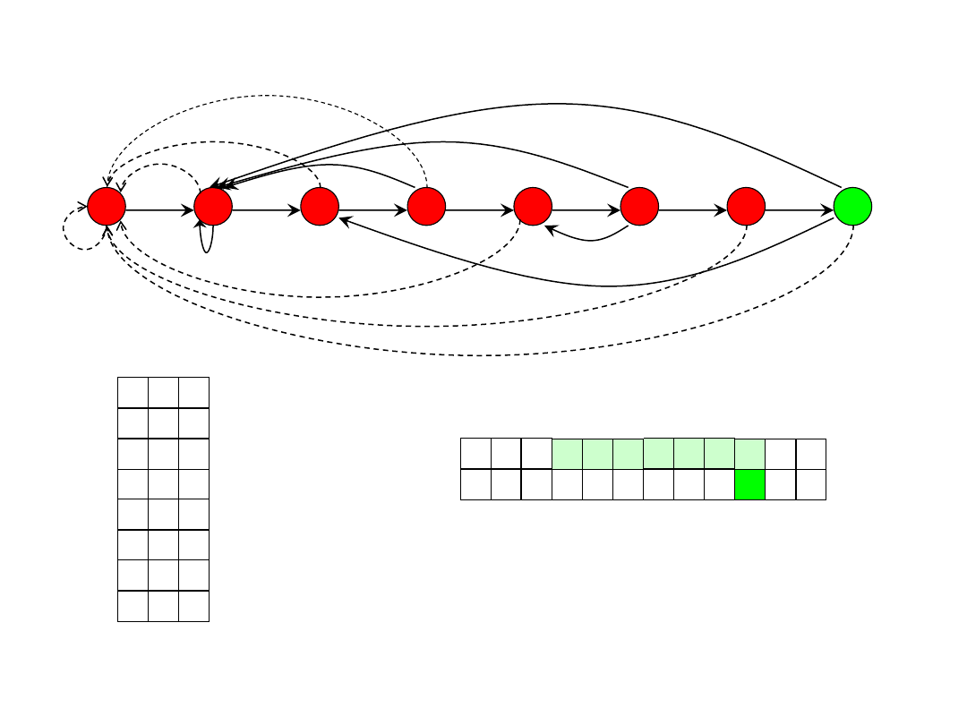
0

7

1

2

3

4

5

6

a

b

a

b

a

c

a

b

b

a

a

a

1 0
1 2

0
1

b

a

d

0
0

c

a
b

P

3 0

2

0 a

1 4

3

0 b

5 0
1 4

4
5

0
6

a

c

7 0

6

0 a

1 2

7

0

9 10 11
a b a
7 2 3

6 7 8
b a c
4 5 6

3 4 5
a b a
3 4 5

- 1 2
- a b

0 1 2

i

T[i]
state

f

(T[i])

b,c

a

c

b,c

c

b,c

b,c

c

15

DSaA 2012/2013

Finite automaton matcher - code

{ 1}
{ 2}
{ 3}
{ 4}
{ 5}
{ 6}
{ 7}

Finite_Automaton_Matcher(T,P)
n := length[T]
q := 0
for i:=1 to n do
q :=

d

(q,T[i])

if q = m then
s := i - m
print „patter occurs with shift” s

{ 1}
{ 2}
{ 3}
{ 4}
{ 5}
{ 6}
{ 7}
{ 8}
{ 9}

Compute_Transition_Function(P,

S

)

m := length[P]
for q:=0 to m do
for a

S

do

k := min(m+1,q+2)
repeat
k := k – 1
until P

k

⊐ P

q

a

d

(q,a) := k

return

d

16

DSaA 2012/2013

Finite automaton matcher - analysis

• The running time of COMPUTE-TRANSITION-

FUNCTION is O(m

3

|

S

|), because the outer loops

contribute a factor of m|

S

|, the inner repeat loop

can run at most m + 1 times, and the test P

k

⊐

P

q

a on line 6 can require comparing up to m

characters.

• Much faster procedures exist; the time required to

compute

d

from P can be improved to O(m|

S

|) by

utilizing some cleverly computed information
about the pattern P. With this improved
procedure for computing

d

, we can find all

occurrences of a length-m pattern in a length-n
text over an alphabet

S

with O(m |

S

|)

preprocessing time and



(n) matching time.

17

DSaA 2012/2013

Knuth-Morris-

Pratt’s idea

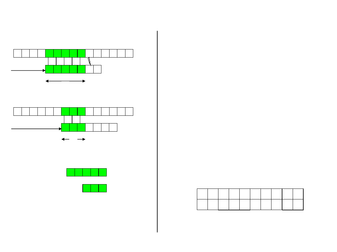
b a c b a b a b a a b c b a b

a b a b a c a

s

q

P

T

b a c b a b a b a a b c b a b

a b a b a c a

s’

k

P

T

a b a b a

a b a

P

q

P

k

?

• Given a pattern P[1..m], the

prefix function for the pattern
P is the function

p

: {1, 2, . . . ,

m}



{0, 1, . . . , m - 1} such

that

p

[q]=max{k: k<q and P

k

⊐ P

q

}

• That is,

p

[q] is the length of the

longest prefix of P that is a
proper suffix of P

q

.

9 10

c a

0 1

6 7 8
b a b
4 5 6

3 4 5
a b a
1 2 3

1 2
a b
0 0

i

P[i]

p

[i]

18

DSaA 2012/2013

KMP - code

{ 1}
{ 2}
{ 3}
{ 4}
{ 5}
{ 6}
{ 7}
{ 8}
{ 9}
{10}
{11}
{12}

KMP_Matcher(T,P)
n := length[T]
m := length[P]

p

:= Compute_Prefix_Function(P)

q :=0
for i:=1 to n do
while q>0 and P[q+1]≠T[i] do
q :=

p

[q]

if P[q+1] = T[i] then
q := q+1
if q=m then
print „patter occurs with shift” i-m
q :=

p

[q]

{ 1}
{ 2}
{ 3}
{ 4}
{ 5}
{ 6}
{ 7}
{ 8}
{ 9}
{10}

Compute_Prefix_Function(P)
m := length[P]

p

[1] := 0

k := 0
for q:=2 to m do
while k>0 and P[k+1]

≠P[q] do

k :=

p

[k]

if P[k+1]=P[q] then
k := k+1

p

[q] := k

return

p

9 10

c a

0 1

6 7 8
b a b
4 5 6

3 4 5
a b a
1 2 3

1 2
a b
0 0

i

P[i]

p

[i]

19

DSaA 2012/2013

KMP - analysis

• The running time of COMPUTE-PREFIX-FUNCTION is



(m), using

the potential method of amortized analysis. We associate a potential
of k with the current state k of the algorithm. This potential has an
initial value of 0, by line 3. Line 6 decreases k whenever it is
executed, since

p

[k] < k. Since

p

[k] = 0 for all k, however, k can

never become negative. The only other line that affects k is line 8,
which increases k by at most one during each execution of the for
loop body. Since k < q upon entering the for loop, and since q is
incremented in each iteration of the for loop body, k < q always
holds. (This justifies the claim that

p

[q] < q as well, by line 9.) We

can pay for each execution of the while loop body on line 6 with the
corresponding decrease in the potential function, since

p

[k] < k.

Line 8 increases the potential function by at most one, so that the
amortized cost of the loop body on lines 5-9 is O(1). Since the
number of outer-loop iterations is



(m), and since the final potential

function is at least as great as the initial potential function, the total
actual worst-case running time of COMPUTE-PREFIX-FUNCTION
is



(m).

• A similar amortized analysis, using the value of q as the potential

function, shows that the matching time of KMP-MATCHER is



(n).