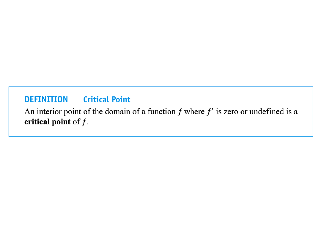
CRITICAL POINTS

monotonicity

Small Review

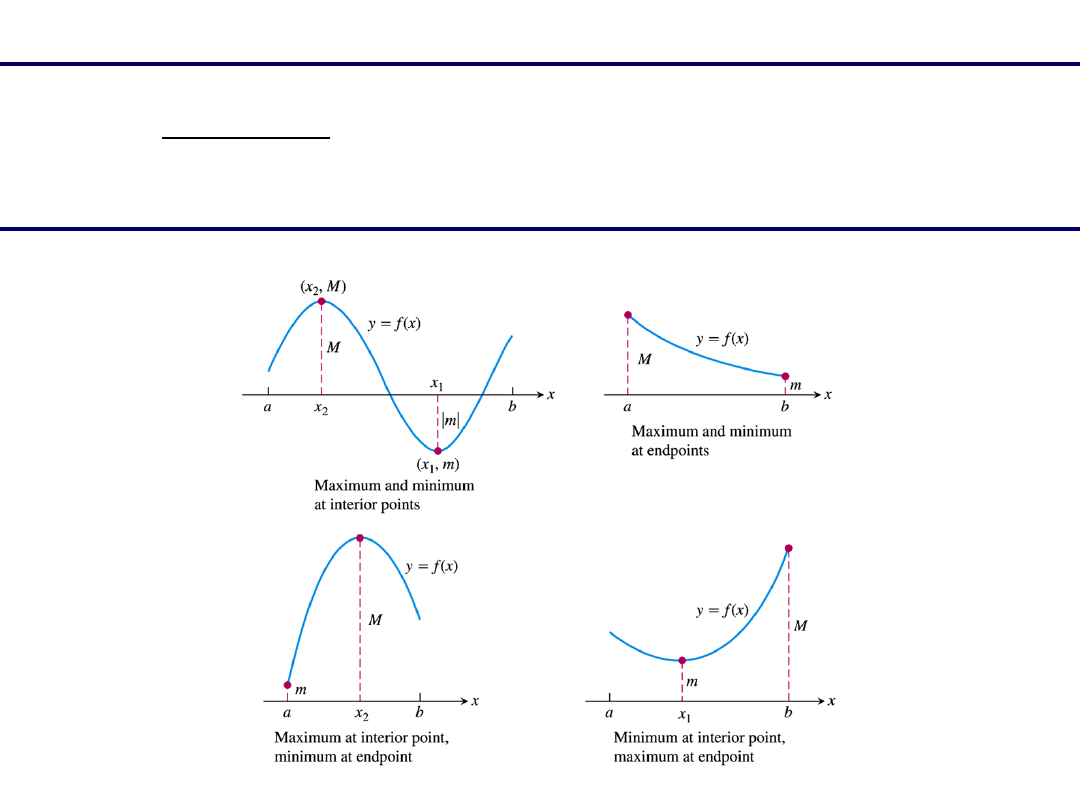
EXTREME VALUE THEOREM (Lecture 3)

Extreme Value Theorem

,

If a function f is continuous on a closed and bounded interval [a,b], then
there exist two points, x

1

and x

2

, in [a,b] such that f (x

1

) = m is the global minimum

of f on [a, b] and f (x

2

) = M is the global maximum of f on [a, b].

Let f (x) be a continuous function in the neighbourhood N

a

of a .

If f (a) > 0 then there exists a neighbourhood M

a

(maybe smaller than N

a

)

of a such that :

0

)

( 





x

f

M

x

a

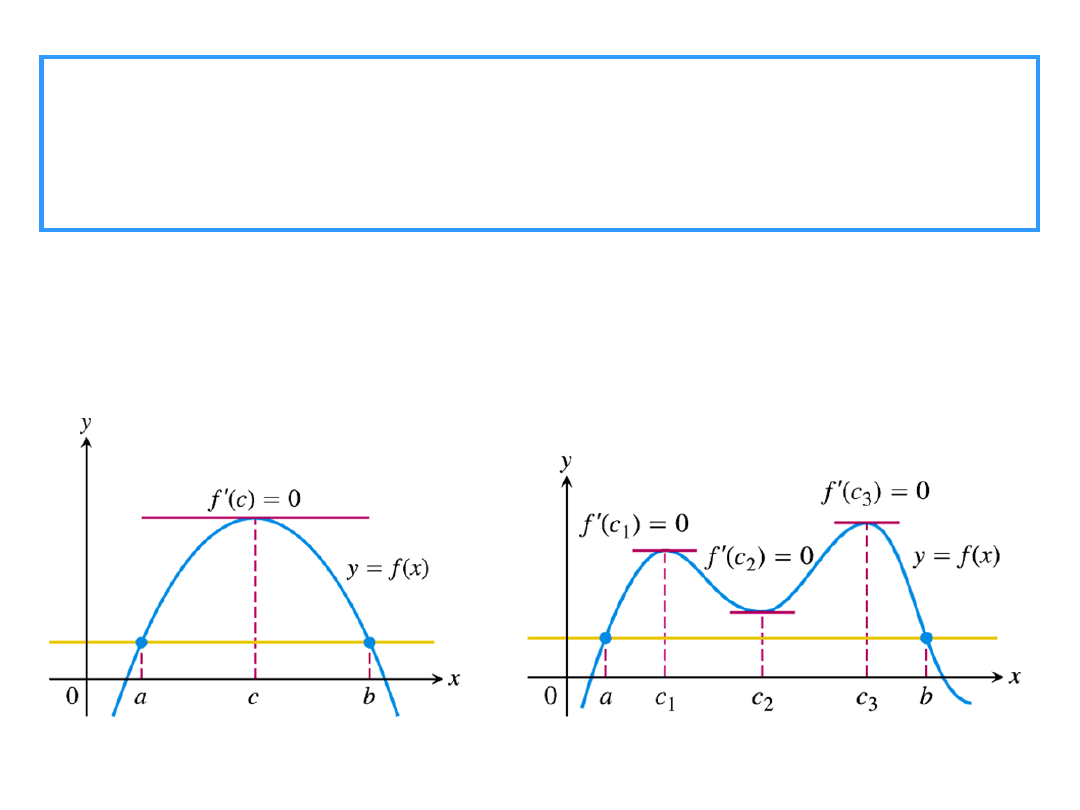
ROLLE'S THEOREM

Suppose that a function f is continuous on a closed and bounded
interval [a,b], differentiable on the open interval (a,b) and f (a) = f (b).
Then there exists some c such that a < c < b and
f’(c) = 0.

Parallel

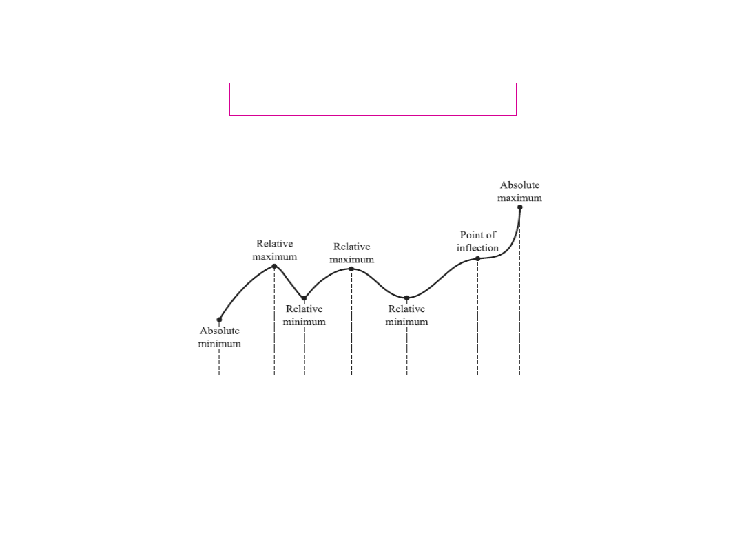
CRITICAL POINTS

On a closed interval [a, b]

Lecture 3

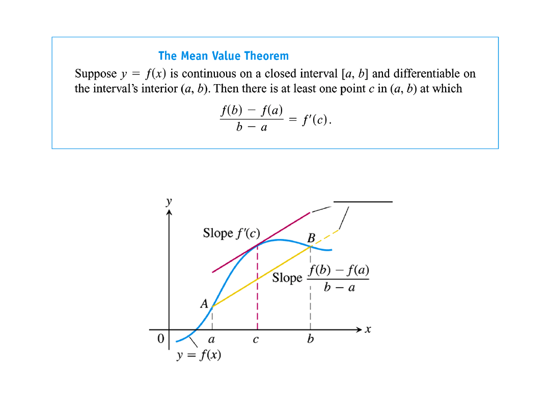
Suppose that the function f is continuous on a closed and bounded
interval [a, b], and differentiable on the open interval (a, b). Then the
following statements are true:

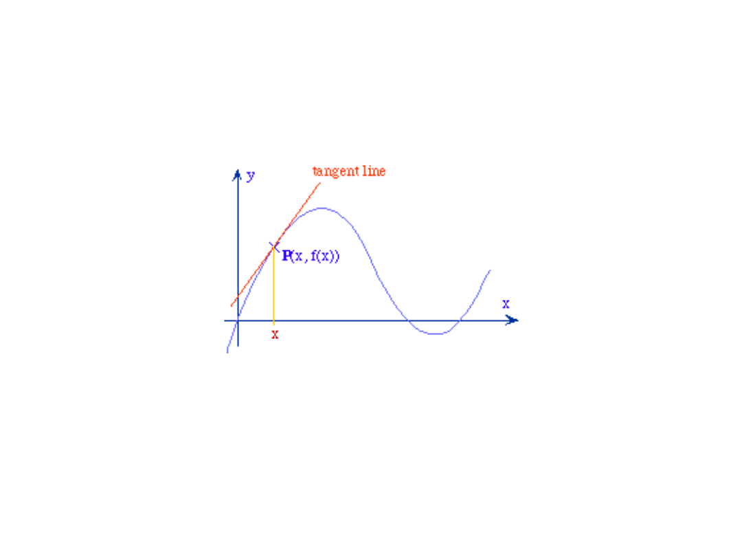
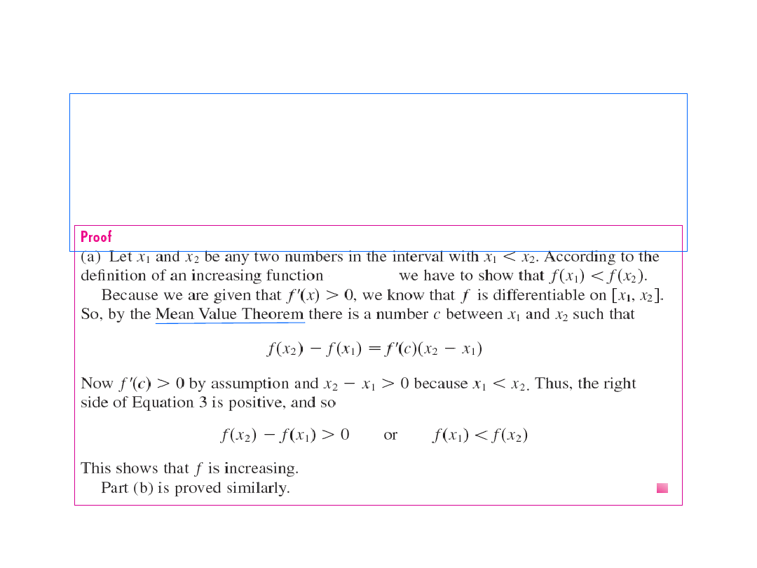
INCREASING / DECREASING TEST

•If f’(x) > 0 for each x in (a,b), then f is strictly
increasing on (a,b).

•If f’(x) < 0 for each x in (a,b), then f is strictly
decreasing on (a,b).

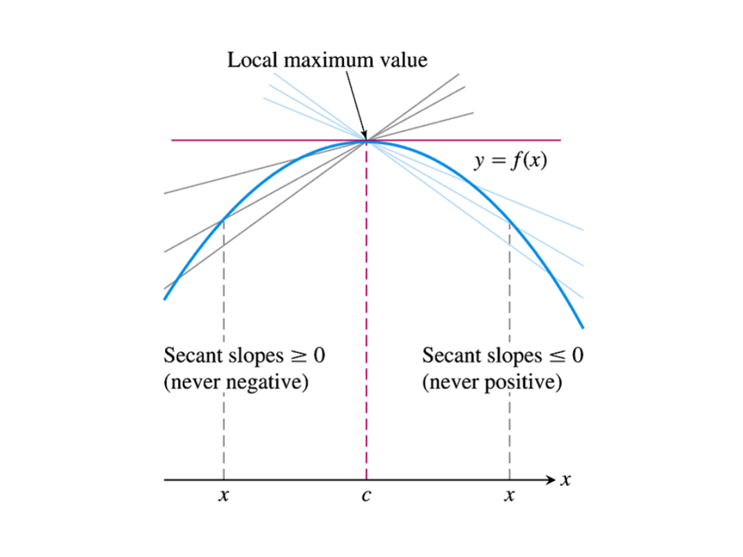
LOCAL EXTREMUM THEOREM

If f is defined on an open interval (a, b) containing c, and f (c)
is a local extremum of f and f’(c) exists, then

f’(c) = 0.

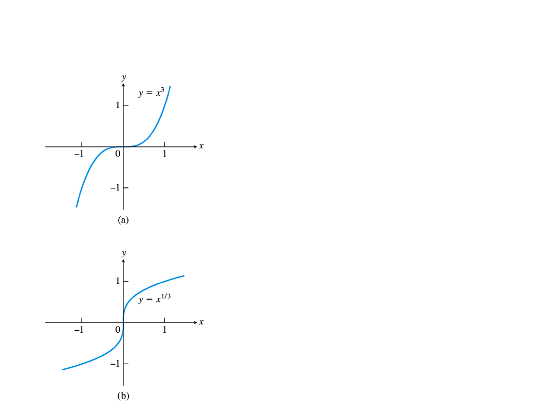
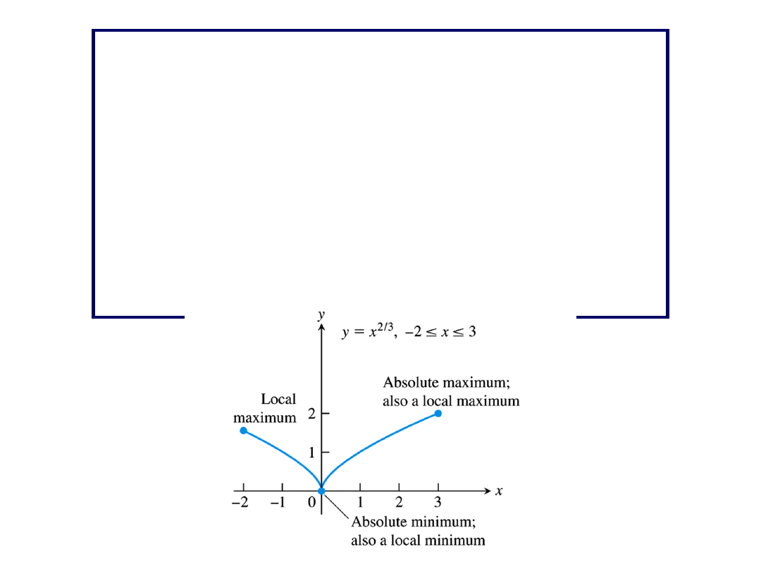
Critical points without extreme values

y’= 3x

2

is 0 at x = 0

y’ = (1/3)x

-2/3

is undefined at x = 0,

but y= x

1/3

has no extremun there.

Suppose that two functions f is contnuous on a closed
and bounded interval [a, b], and differentiable on the
open interval (a, b). Then the following statements are
true:

•If f’(x) > 0 for each x in (a,b), then f is strictly
increasing on (a,b).

•If f’(x) < 0 for each x in (a,b), then f is strictly
decreasing on (a,b).

•If f’(x) > 0 for each x in (a,b), then f is increasing on
(a,b).

•If f’(x) < 0 for each x in (a,b), then f is decreasing on
(a,b).

•If f’(x) = 0 for each x in (a,b), then f is constant on
(a,b).

Show that

1

1

1

1

2

ln

.

2

1

,

1

1

3

2

.

1

0

0



















x

x

for

x

x

x

x

x

for

x

x

THE FIRST DERIVATIVE TEST for extremun

Let f be continuous on an open interval (a, b), and a < c < b:

(i) If f’(x) > 0 on (a, c) and f’(x) < 0 on (c, b), then f (c) is a local
maximum of f on (a,b).

(i) If f’(x) < 0 on (a, c) and f’(x) > 0 on (c, b), then f (c) is a local
minimum of f on (a,b).

CRITICAL POINT THEOREM

Let f be continous on its domain I. Suppose that c
is a point in I
and has either a maximum or a minimum at c. Then
one of the
following three things must happen:

(i) c is an end point of I
(ii) f’(c) is undefined
(iii) f’(c) = 0

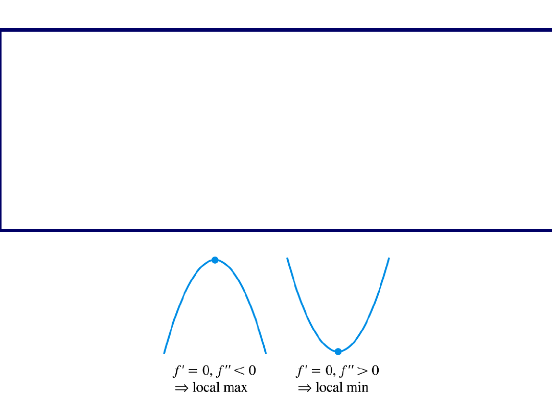
THE SECOND DERIVATIVE TEST

Suppose that f, f’ and f’’ exist on an open interval (a, b) and a<c<b.
Then the following statements are true:
(i) If f’(c) = 0 and f’’(c) < 0, then f (c) is a local maximum of f.
(ii) If f’(c) = 0 and f’’(c) > 0, then f (c) is a local minimum of f.
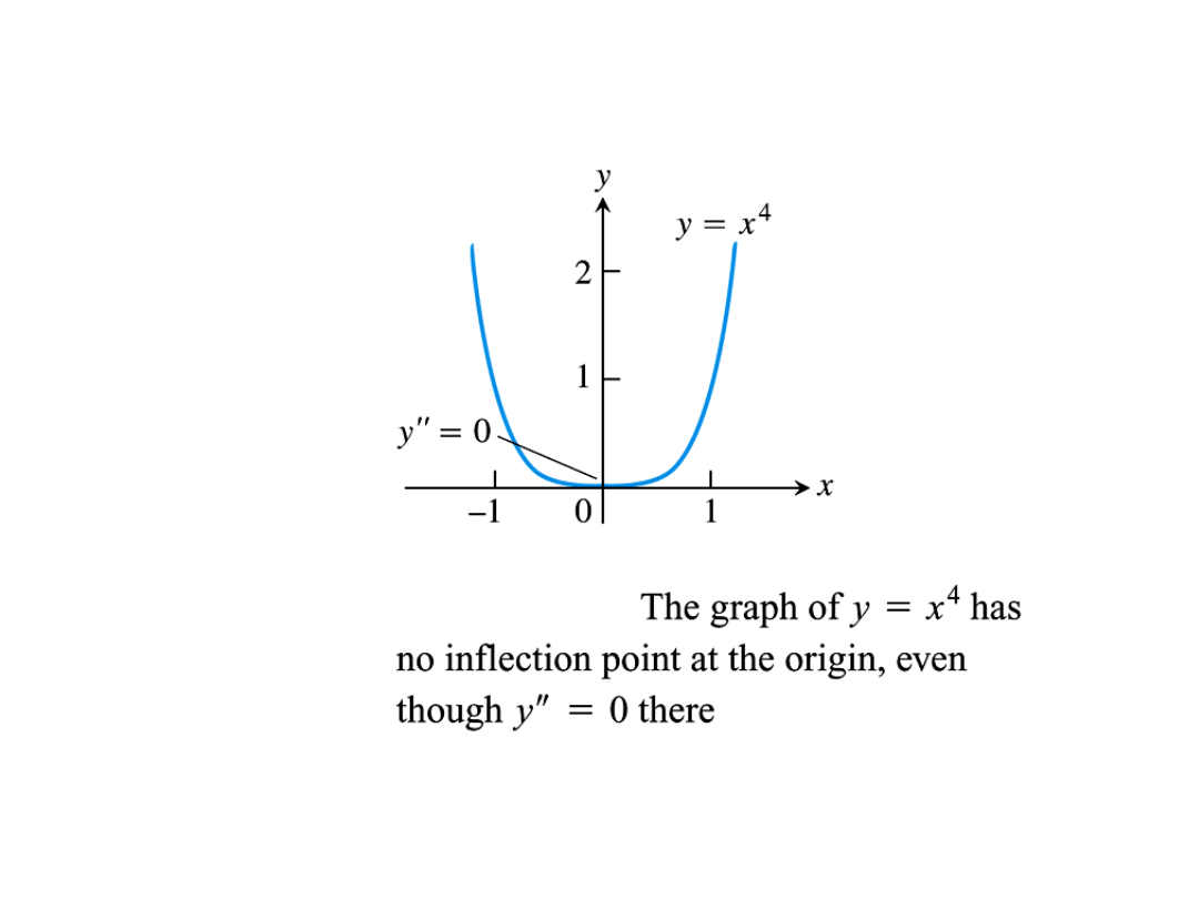
(iii) If f’(c) = 0 and f’’(c) = 0, then f (c) may or may not be a
local extremum of f.

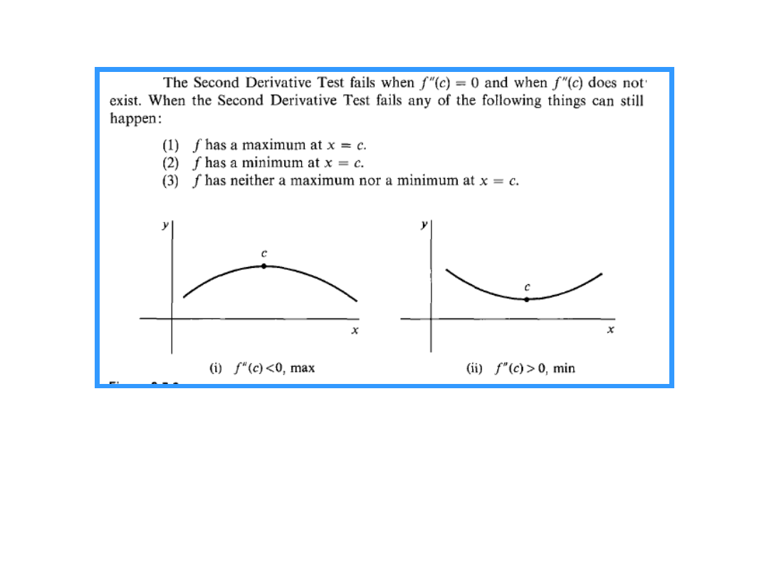
Then we test for ....

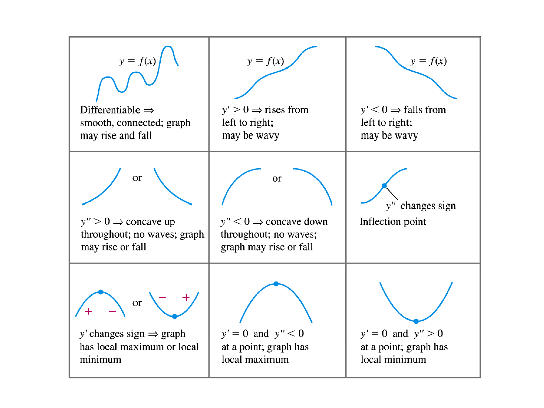
CONCAVITY, CONVEXITY,

INFLECTION POINTS

CONCAVITY, CONVEXITY, INFLECTION POINTS

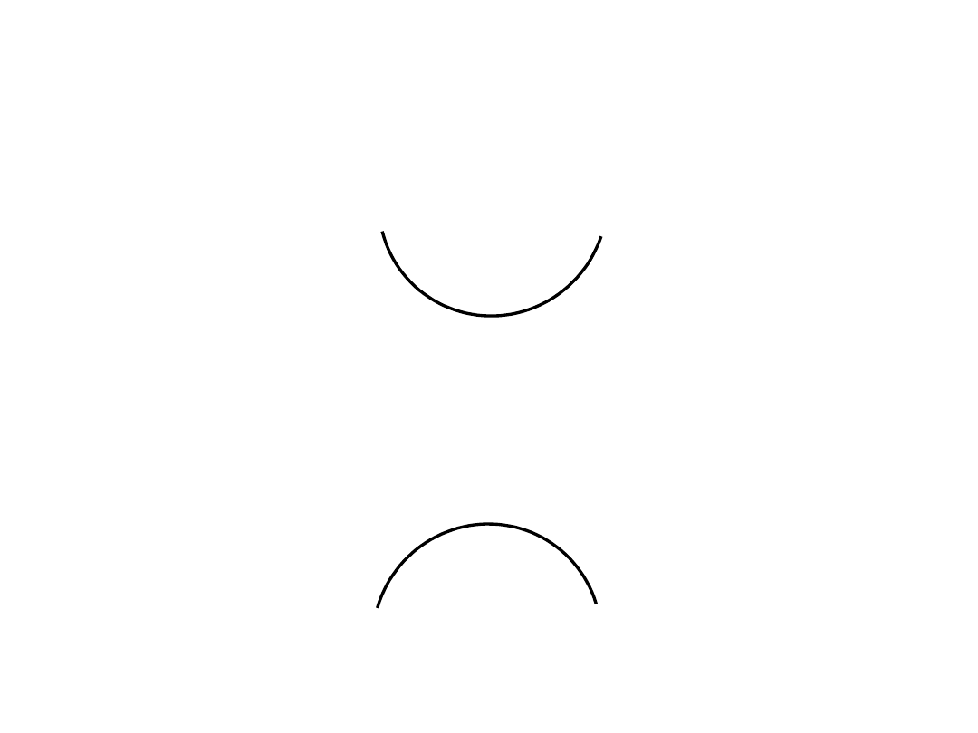
A piece of the graph of f is convex (concave upward) if
the curve 'bends' upward. For example, the popular
parabola y = x

2

is convex (concave upward) in its entirety.

CONVEX

CONAVE

A piece of the graph of f is concave (concave downward)
if the curve 'bends' upward. For example, a flipped
version the popular parabola y = - x

2

is concave

(concave downward) in its entirety.

f (λx

1

+ (1-λ)x

2

) ≤ λ f (x

1

) + (1-λ) f (x

2

).

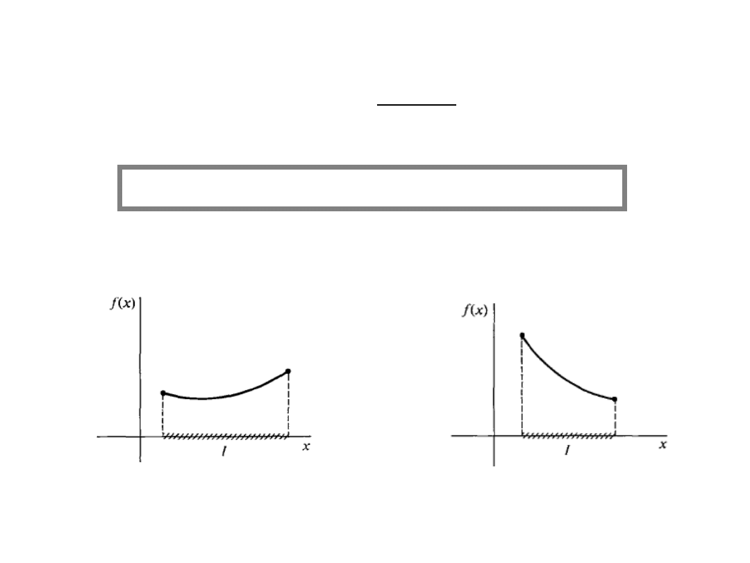
convex, increasing

convex, decreasing

DEFINITION

We say that a function f is convex in an interval P, if
for any numbers x

1

, x

2

in P and for any number λ, 0 < λ

< 1 the following condition is satisfied

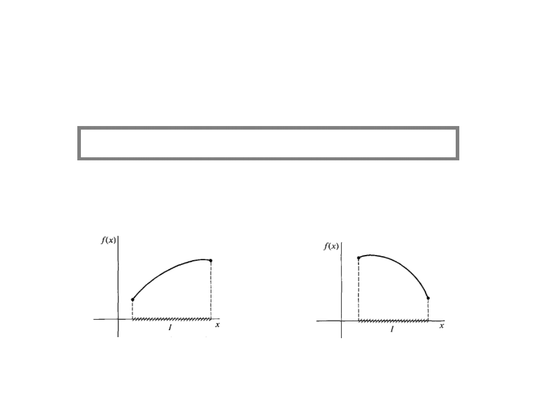
DEFINITION

We say that a function f is concave in an interval P, if
for any numbers x

1

, x

2

in P and for any number λ, 0 < λ <

1 the following condition is satisfied:

f (λx

1

+ (1-λ)x

2

) ≥ λ f (x

1

) + ( 1-λ) f (x

2

).

concave, increasing

concave, decreasing

Theorem

Assume a function f is continuous in an interval P and twice
differentiable in the interior of P i.e. (a,b). The function f is

convex

in an interval P if, and only if

f '' (x) ≥ 0

for every x

from (a,b).

strictly convex

in an interval P if, and only if

f '' (x) > 0

for

every x from (a,b). and f ''  is not a null-function on any
subinterval of P;

concave

in an interval P if, and only if

f '' (x) ≤ 0

for every x

from (a,b).

strictly concave

in an interval P if, and only if

f '' (x) < 0

for

every x from (a,b) and f ''  is not a null-function on any
subinterval of P .

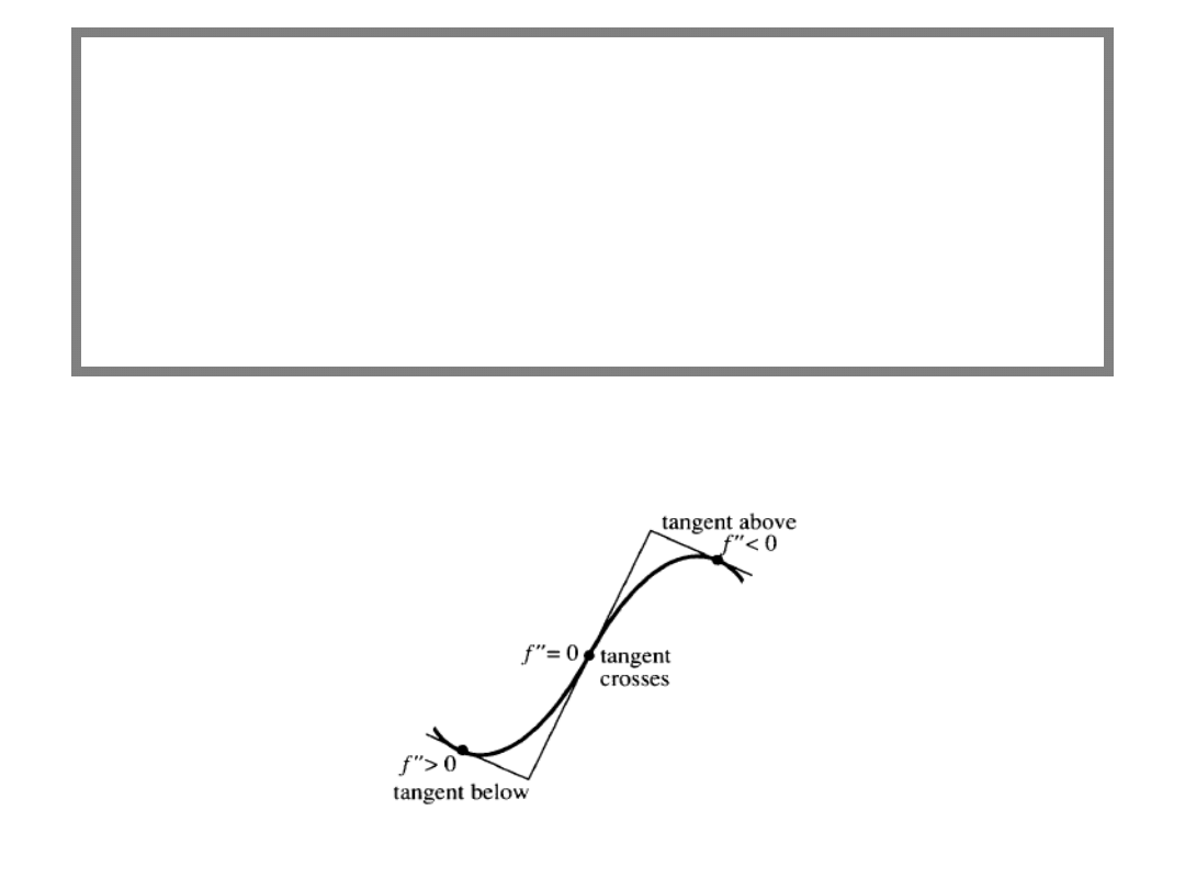
INFLECTION POINTS

Definition

Let a function f be defined on some neighborhood of a
point x

0

. We say that a point (x

0

, f (x

0

)) is an inflection

point of the function f, if there exists a number δ > 0 such
that on one of the intervals (x

0

, x

0

+ δ) or (x

0

- δ, x

0

) the

function f is strictly convex, and on the second one it is
strictly concave.

i.e. a point where the graph of a function has a tangent line and where the
concavity changes.

HIGHER ORDER DERIVATIVES AND EXTREMA OF A FUNCTION

Theorem

Let f be a function defined in some neighborhood of a point x

0

.

Let

1. if

n is even

, then f has extremum at x

0

and:

(a) if f

(n)

(x

0

) > 0, then f has a

minimum

at x

0

,

(b) if f

(n)

(x

0

) < 0, then f has a

maximum

at x

0

.

2. if

n is odd

, then f has no extremum at x

0

but f does have an

inflection point

at x

0

.

.

1

n

,

0

)

x

(

and

0

)

x

(

)

x

(

)

x

(

'

0

(n)

0

)

1

n

(

0

0















f

f

"

f

f



CURVE SKETCHING

One has to:
1. Determine the domain;
2. Determine the intersection points of the graph of the

function with the axes, check out the periodicity of the
function;

3. Compute either the limits or values of the function at the

end points of intervals of which the domain consists;

4. Determine the asymptotes;
5. Compute the derivatives of the function, and determine

intervals of monotonicity as well as relative extrema;

6. Compute the second derivative of the function , and

determine the intervals of convexity as well as the
inflection points;

7. Compute the values of the function at the of extremal and

inflection points;

8. Sketch the graph of the function (results of points 1 - 7 may

be summarized in a table).

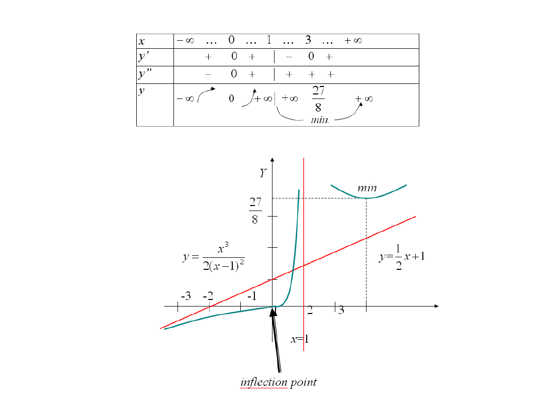
Sketch a graph of the function

1. The

domain

: X=

2. Values at

endpoints

of domain and x,y-intercepts

3.

Asymptotes

:

The function has a

vertical

asymptote

x=1

Slant asymptotes:

Both of the

slant asymptotes

are given by the equation

 

2

3

)

1

(

2 



x

x

x

f

)

,

1

(

)

1

,

(















y

x

lim









y

x

lim









y

x 1

lim









y

x 1

lim

2

1

)

(

lim

2

1

)

(

lim

















m

x

x

f

x

x

f

x

x

1

2

1

)

1

(

2

lim

1

2

1

)

1

(

2

lim

2

3

2

3

















































k

x

x

x

x

x

x

x

x

1

2

1



 x

y

 













)

3

(

)

1

(

2

1

1

2

1

3

2

1

3

2

4

3

2

2





















x

x

x

x

x

x

x

x

x

f

 

3

,

0

0

'

)

2

1







x

x

for

x

f

a

 

 

3

0

'

3

0

'









x

dla

x

f

x

dla

x

f

8

27

)

3

(

min



 f

y

 

)

,

3

(

)

1

,

0

(

)

0

,

(

0

'

)













x

dla

x

f

d

 

),

3

,

1

(

0

'

)





x

dla

x

f

e

3

.

The first derivative

b) at x

1

= 0

there is no extremun

, because f



(x) >0 in the neighbourhood

of x

1

= 0 ( f



(x) does not change sign).

c) at x

2

= 3 there is a

minimum

, because

the

function decreases

the

function increases

4.

The second derivative

 

4

)

1

(

3

"





x

x

x

f

 

 

 

)

,

1

(

0

"

)

1

,

0

(

0

"

0

)

0

(

"

)

0

,

(

0

"



















x

dla

x

f

x

dla

x

f

f

x

dla

x

f

)

0

,

(

The function is

convex

for

)

,

1

(

)

1

,

0

(







The function is

concave

for

The point (0, 0) is the

inflection point

.

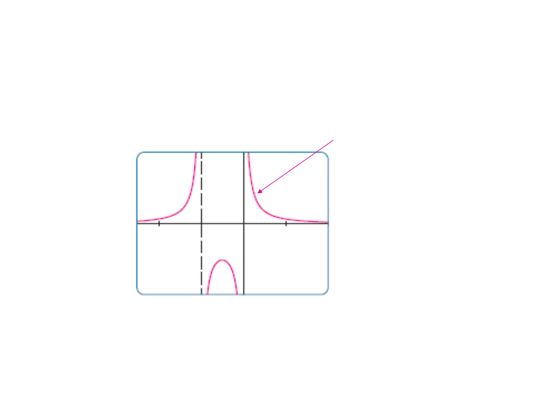
Write a proposed equation of the sketched function

f (x) = ?

1

-1

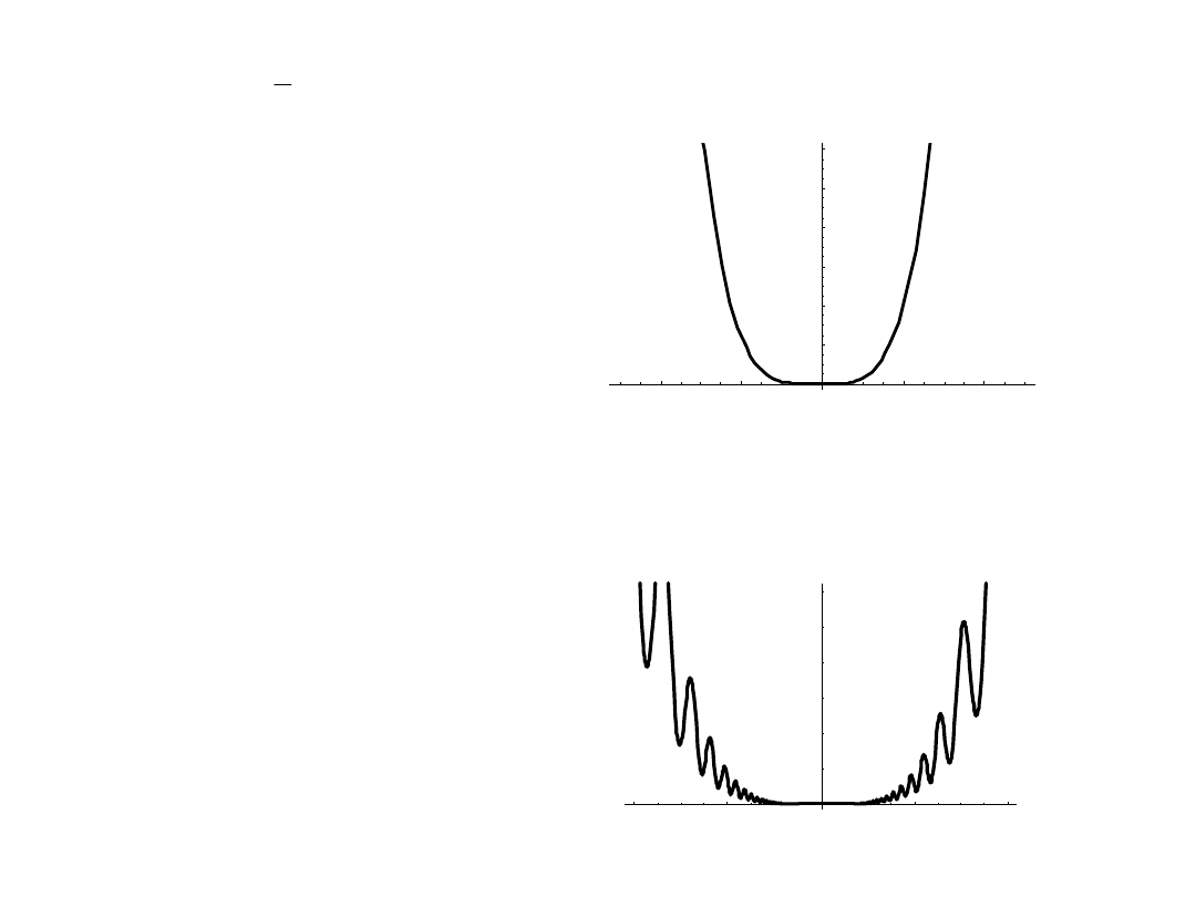
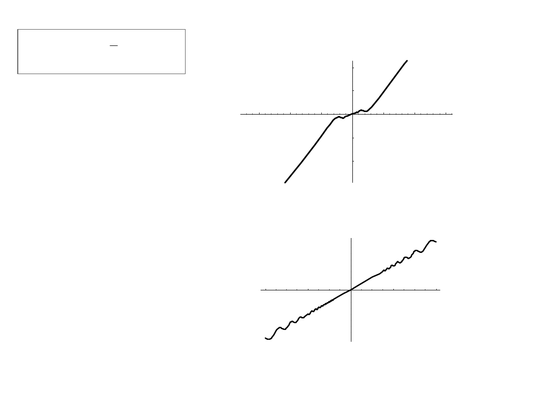
Peculiar Examples

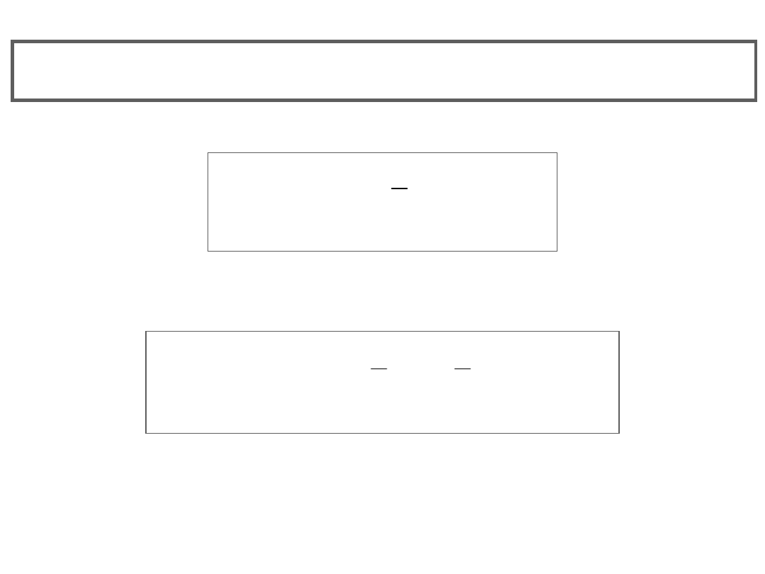
A differentiable function having an extreme value at a point where
the derivative does not make a simple change in sign.























 



0

x

if

0

0

x

if

x

1

sin

2

x

)

x

(

f

4

has an absolute minimum at x = 0. Its derivative is





































 



0

x

if

0

0

x

if

x

1

cos

x

1

sin

2

x

4

x

)

x

(

'

f

2

which has both positive and negative values in every neighbourhood
of the origin. In no interval (a,0), (0,b) is f monotonic.























 



0

x

if

0

0

x

if

x

1

sin

2

x

)

x

(

f

4

)

5

,

5

(

x





)

04

.

0

,

004

.

0

(

x





-4

-2

2

4

20

40

60

80

100

120

-0.04

-0.02

0.02

0.04

510

- 7

110

- 6

1.5 10

- 6

210

- 6

2.5 10

- 6

310

- 6

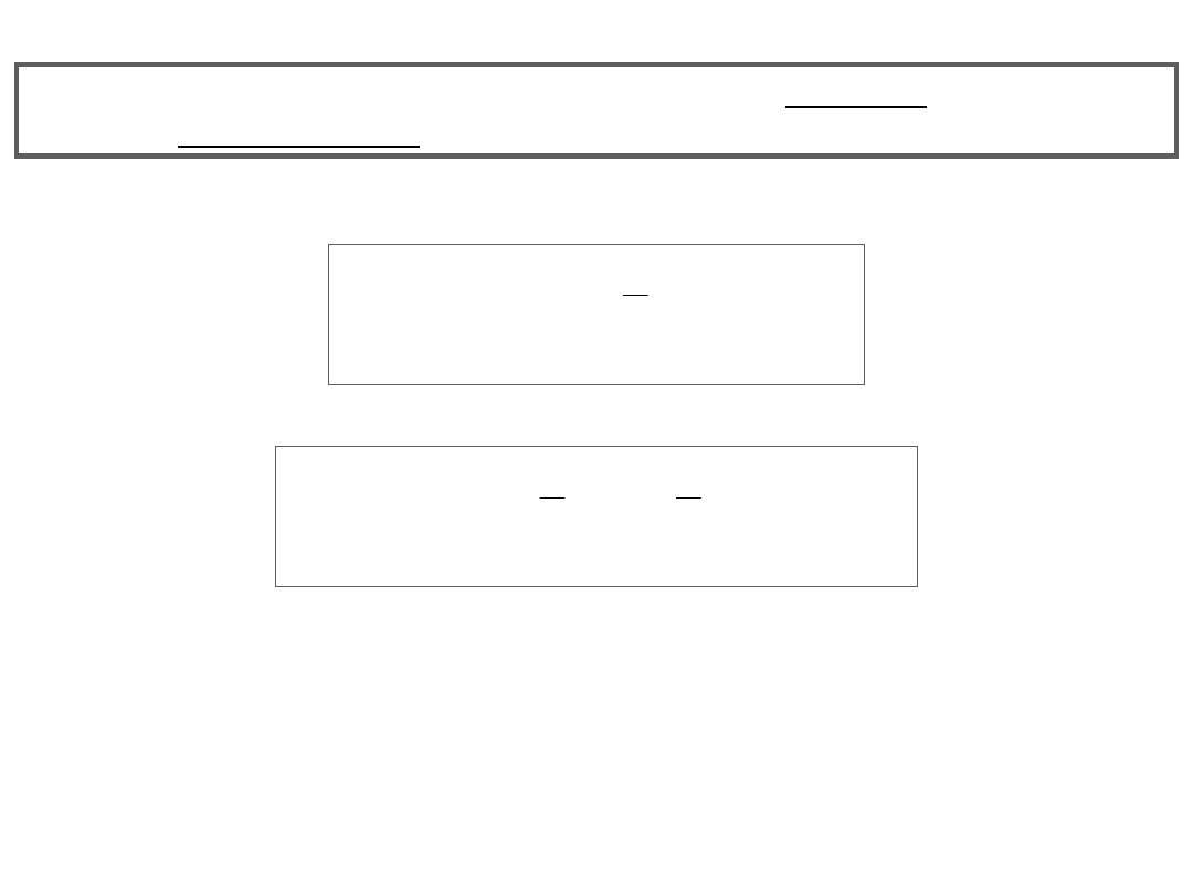
A differentiable function whose derivative is positive at a point but
which is not monotonic in any neighbourhood of the point.

















0

x

if

0

0

x

if

x

1

sin

x

2

x

)

x

(

f

2



















0

x

if

0

0

x

if

x

1

cos

2

x

1

sin

x

4

1

)

x

(

f

In every neighbourhood of 0 the function f’(x) has both positive and
negative values.

-1.5

-1

-0.5

0.5

1

1.5

-2

-1

1

2

)

5

,

5

(

x





-0.04

-0.02

0.02

0.04

-0.04

-0.02

0.02

0.04

)

04

.

0

,

004

.

0

(

x





















0

x

if

0

0

x

if

x

1

sin

x

2

x

)

x

(

f

2

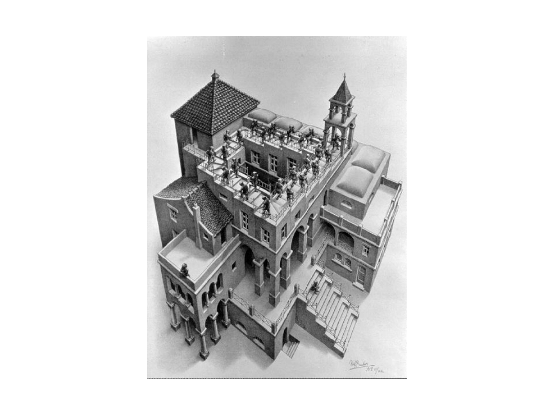
Ascending and Descending

M. C.
Escher
1960

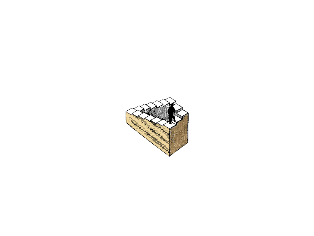
NO EXTREMA