markov v1 artykul

Latent Markov Chain Analysis of Income

States with the European Community

Household Panel (ECHP). Empirical Results

on Measurement Error and Attrition Bias.

∗

Edin Basic

Freie Universität Berlin

Ulrich Rendtel

Freie Universität Berlin

June 2004

Paper presented at the 2nd International Conference of ECHP Users

- EPUNet 2004 Berlin, June 24-26, 2004

∗

Support by Statistics Finland for data access is gratefully acknowledged. Special thanks to

Johanna Sisto and Marjo Pyy-Martikainen of Statistics Finnland for their help in the compilation
of all the necessary information to run our data analysis.

Introduction

In examining dynamic aspects of poverty, economists and other social scientists
have focused their attention on panel data. Information on individual income his-
tories can be used for conclusions about the persistence of poverty. These con-
clusions, however, can be affected by measurement error and non-response. In
the European Community Household Panel (ECHP) some countries use income
data from the questionnaire while others with national registers use information
collected from administrative records. The existence of survey-based and register-
based income information for the same persons provides a unique opportunity to
study how sensitive measures of income mobility are with respect to the under-
lying data source. If these two income measurements lead to the same sequence
of poverty states this provides evidence for a true change between poverty states.
In the case of non-corresponding poverty sequences one would conclude that the
measurement error is present. Furthermore, if the register income is taken to be the
"true" income, the measurement error can be directly identified. The effect of non-
response can be examined using information from register also for non-responding
persons. In this paper we investigate transition tables between subsequent income
states. Latent Markov chain models are used to model incorrect classification of
income states. These models assume, in a probabilistic way, that the observed
(manifest) variables are imperfect reflections of another set of variables that are
unobserved (latent). The observed variables are linked to the unobserved by re-
sponse matrices that represent the probabilities to observe the manifest categories
for different latent categories. In addition transitions in behavior occur among
latent variables and they are described by another matrix of Markov transition
probabilities.

The data we use in this analysis come from the first five waves of the Finnish

European Community Household Panel (FIN-ECHP) and cover the years 1995,
1996, 1997, 1998 and 1999.

The paper is organized as follows: Section 2 gives a brief description of the

data we used in our analysis. In Section 2.1 we define the applied income con-
cepts, since section 2.2 gives the potential sources of income measurement error in
surveys. In Section 2.3 we define the poverty lines used here. Section 3 compares
the mean incomes and the shape of the distribution for both income measure-
ments. Section 4 presents a comparison of the observed transition tables between
the poverty states. Then we introduce the latent Markov models and report our
estimation results for these models. In Section 6 we give a brief description of
panel attrition and asses the effect of panel attrition on the estimates of income
mobility. Section 7 concludes.

The Data

The European Community Household Panel (ECHP) is a standardized multi-purpose
annual longitudinal survey carried out at the level of the European Union.

started in 1994 and is centrally designed and coordinated by the Statistical Offices
of the European Communities (Eurostat). A sample of 60 000 households in 12
countries was identified that year. Another 13 000 households have been added
since Austria, Finland and Sweden joined the ECHP. Every year a new panel wave
was launched. The main subjects of this survey were information on household
income and living conditions in the European Union because of the comparability
of the data generated as well as the multidimensional coverage and the longitu-
dinal design of the instrument which allows the study of changes over time at
the micro level.

Comparability in time is achieved by keeping the interval be-

tween successive waves close to twelve months and by keeping to a minimum the
changes to the ECHP questionnaire from one wave to another.

In Finland, the ECHP has been conducted yearly since 1996 by Statistics Fin-

land. The income data in the Finnish-ECHP are primarily based on statistical reg-
isters drawn from administrative records.

However, in the first wave of the Finish

ECHP in 1996 the data on incomes were also collected in the same way as in most
of the other participating countries i.e. by personal interviews. This was repeated
in the fifth wave in 2000. The principal accounting period for income employed
in the ECHP is the previous calendar year i.e. the income data in 1996 and 2000
is related to calendar 1995 and calendar 1999 respectively. For these two years it
was possible to match the survey data with register data at the individual level by
a personal identification number. We restrict our analysis to persons of at least 16
years which were marked as sample persons. Sample persons are all individuals
belonging to the first wave in the FIN-ECHP. Sample persons are eligible for an
interview if they are aged 16 or older and belong to the target population (that is,
they live in a private household within the EU). The resulting sample consists of
5570 persons.

For the analysis of nonresponse we only took the data from waves 1996 and

2000 into account and split the full sample (with attriters and respondents) in
1996 into samples of attriters and respondents, according to the response behavior
in 2000. We obtained an attrition rate of 24 % between 1996 and 2000.

See Peracchi [2002], p.64.

See Eurostat [2000], p.4.

See Nordberg et al., [2000].

2.1

Definition of income concepts

The interview-based estimate of total household income is calculated as the unad-
justed sum of all (net) incomes reported by all members of the household during
the interviews.

The register-based estimate of total household income is obtained

in the same way by adding all incomes found in the registers for all members of
the interviewed households and by using as far as possible the same income con-
cepts as in the interviews.
For purposes of our analysis we used the household equivalence income. The
household equivalence income is calculated as a function of the number of house-
hold members, taking into account the fact that household composition can change
over time and that households share common services and thus may enjoy some
degree of economies of scale in consumption. Here we used the OECD scale,
that gives weight 1 for the head of the household and weight 0,5 for other adults,
while children younger than 14 receive the weight 0,3. This income illustrates the
household’s welfare position controlled for household size and structure and is
assigned to all members of the household. The household composition was taken
from the survey at the time of the interview.

In all comparisons reported below the unit of the analysis is the individual. The

use of individuals as a unit of analysis has some advantages, e.g. when assessing
the extent of poverty, larger families receive greater weight than smaller families
or the poverty status of individuals can be traced over time, whereas it is often
unclear how to define changes over time in the poverty status of family units when
family structure changes (e.g. through marriage or divorce).

2.2

Sources of income measurement error in surveys

In the following section we discuss potential sources of measurement error in
income surveys.

With measurement error we mean discrepancies between the

true respondents income (e.g. income from administrative records) and his or her
reported income.

• There is a tendency to forget to report small incomes (e.g., earned from the

second or third job held).

• In the case of uncertainty about income the respondents may deliberately

give a conservative estimate or an estimate known from previous years.

• In the survey the interviewees may also report irregular incomes which are

not considered in the income from administrative data.

See Nordberg et al., [2000].

See Rendtel et al., [2003].

• The respondents may misunderstand the income question e.g. report gross

instead of net income.

• In the case of self-employment and investment income the respondents have

a tendency to misreport due to lack of knowledge (this may be quite legiti-
mate when a respondent leaves his financial affairs to an accountant).

• Because of the retrospective way of data collection (i.e. the information on

income refers to last calendar year) the respondent may have difficulties to
recall the exact amount of annual income and give an estimate which would
not coincide with the income from administrative records.

All of those points would tend to lead to either an over- or underestimation of

income.

2.3

Definition of the poverty states

A key choice in defining poverty is the specification of the income threshold below
which persons are classified as being poor. There are two different concepts in
defining poverty: absolute and relative poverty. In this study we use a relative
poverty threshold, which is set to an income equal to half the median income. This
means that the individuals are included in the poverty population if their available
income is lower than the half of the median equivalence income. We also use
a more informative quintiles description of poverty. Absolute poverty standards
are commonly used in the context of developing countries and absolute poverty is
defined as having an income below the minimum resources required to live at a
certain level of welfare. In the following analysis we defined the observed income
states in accordance of their respective measurement, i.e. a person is regarded
as "poor by register" if the register equivalence income is less than 50 percent of
the median register income. The state "poor by survey" is defined analogously by
using the survey income and the poverty line defined by the survey income. The
same approach was also used for quintile income states.

Comparison of the Distribution

In order to find out whether there are any discrepancies between the register and
survey equivalence income, we compare the distribution of income for both mea-
surements. Table 1 shows the mean equivalence income per quintile in 1996 and
2000 for the two income measurements when individuals are ordered according
to their equivalence income as estimated from register.

Table 1:

Mean equivalence income (in Finmark FIM) per quintile in 1996 and 2000.

Mean income (FIM)

1996

2000

Survey

Registers

Diff.(%)

Survey

Registers

Diff.(%)

Quintile

(1)

(2)

100

(1)−(2)

(2)

(3)

(4)

100

(3)−(4)

(3)

44 980

45 712

-1.6

58 760

56 596

+3.8

57 611

63 740

-9.6

68 475

71 403

-4.1

68 449

77 427

-11.6

82 473

88 765

-7.1

80 537

93 622

-13.9

96 198

109 909

-12.5

110 956

143 513

-22.6

143 469

186 229

-22.9

All

72 507

84 749

-14.4

89 875

102 580

-12.3

Included are only persons who participated in both waves

Comparisons of mean incomes (Table 1) show that there is a clear underre-

porting of equivalence incomes. The tendency of underreporting is especially
clear in the upper tail of the income distribution (in the upmost quintile the under-
reporting is over 20 per cent for both years). For both years there is a tendency
to higher underreporting from the lowest quintile to the highest quintile and also
a small downward trend in the overall underreporting when comparing the results
for 1996 and 2000 (the underreporting decreased from -14.4 per cent to -12.3 per
cent). This may be interpreted that the survey income becomes more reliable i.e.,
the respondents become more familiar with income questionnaire over time and
consequently they make less mistakes in the reporting their incomes.

Now we compare the shape of the distribution of the register-based and survey-

based equivalence income. Figure 1 and 2 display a kernel density estimate of the
1996 and 2000 income distributions. It appears that the distribution of both in-
comes is unimodal, most of the incomes clustering in the middle-income class.
For both years (1996 and 2000) register measurement (solid line) is shifted to
higher values than the corresponding survey measurement (dotted line). Such a
view would support the assumption that the respondents underreport their income.
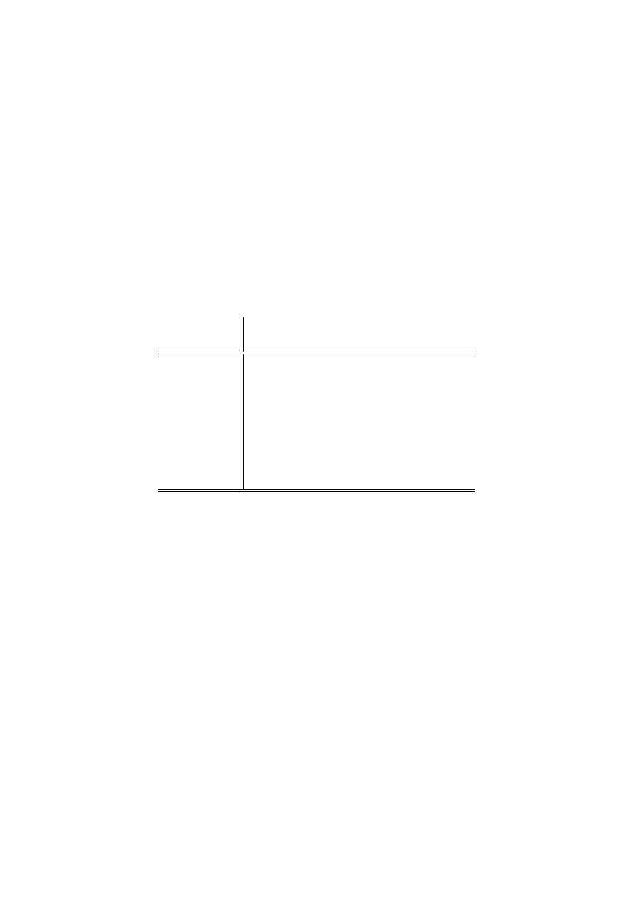
Figure 3 presents the distribution of the differences between survey income and

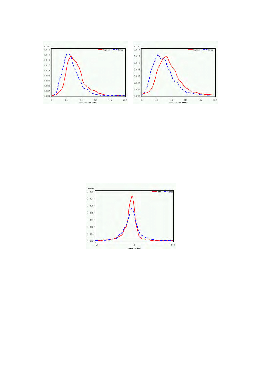
Figure 1:

The Distribution of household equivalence income in 1996 and 2000.

register income for the years 1996 and 2000. The general shape of these dis-
tribution appears to be quite stable over time. The gross of the distribution is
concentrated in the negative range, which means underreporting of the survey
income. However, Figure 3 shows that there is no systematic ordering of two in-
come measurements and demonstrates that for all points in time the ordering of
the two measurements is reversed for some part of the sample. The proportion of
observations where this is true changes slightly over time.

Figure 2:

The Distribution of the Differences between register and survey

household equivalence income in 1996 and 2000.

3.1

Comparison of observed transition tables between income
states

The most interesting use of panel data is the analysis of change. We use here tran-
sitions between poverty states (Table 2) and transitions between quintiles (Table
3) of the equivalence income. A comparison of the starting distribution in Table
2 reveals that the percentage of poor persons is considerably higher with the use
of the survey income. In general the transition matrices for the survey income
indicate a higher instability. The risk to fall from non-poverty into poverty is 60
percent higher for the survey income. The same holds for the risk to move from
the upmost quintile to the lowest quintile within four years in Table 3. On the
opposite side, the risk to stay in poverty is almost the same for the register and the
survey income. The risk to stay in the lowest quintile is decreased by the factor of
a 0.8 if we switch from the register to the survey measurement. However, as we
will see later, if we take both measurements as not precise measurements of the
true income state, the mobility between the true states is greatly overstated by the
figures in Tables 2 and 3.
The larger instability of the survey income may simply result from higher noise
in the measurement by the survey. If the measurement errors in 1996 and 2000
are independent from each other this results in an increased variability of tempo-
ral differences. As a consequence, we will observe higher risks to jump between
more distant income states. Therefore the measurement error results in a system-
atic bias for measures of stability. This is what we observed in Tables 2 and 3.

Table 2:

Comparison of transitions between the states "Poor" and "Non-poor" for

survey and register income. Time interval: 1996 to 2000.

Transitions in percent

Start

Poor

Not poor

3.91

31.65

68.34

Poor

(0.3)

(3.2)

(0.3)

96.8

5.34

94.65

Not Poor

(0.3)

(3.2)

(0.3)

Survey

7.56

30.40

69.59

Poor

(0.4)

(2.2)

(0.4)

92.44

8.66

91.33

Not Poor

(0.4)

(2.2)

(0.4)

Standard Errors in Parenthesis

Table 3:

Comparison of transitions between quintiles of the household equivalence

income for survey and register income. Time interval: 1996 to 2000.

Survey

2000

Quintiles

1996

51.10 25.10 13.40 7.00

3.50

41.50 27.70 13.60 7.40

8.80

(1.4)

(1.2)

(1.0)

(0.7)

(0.5)

(1.4)

(1.3)

(1.0)

(0.9)

(0.8)

23.80 39.90 21.90 14.70 4.70

22.20 32.90 23.90 15.50 8.40

(1.2)

(1.4)

(1.2)

(1.0)

(0.5)

(1.2)

(1.3)

(1.2)

(1.0)

(0.8)

12.80 21.30 36.00 20.70 11.10 16.10 20.00 28.40 21.00 14.40

(0.9)

(1.2)

(1.4)

(1.1)

(0.9)

(1.1)

(1.2)

(1.3)

(1.2)

(1.0)

8.40

9.40

21.00 39.20 22.00 10.50 13.00 22.80 32.50 22.20

(0.8)

(1.2)

(1.4)

(1.2)

(0.9)

(1.1)

(1.3)

(1.2)

6.90

6.60

8.50

20.00 60.00 10.50 11.10 11.10 22.40 46.00

(0.7)

(0.8)

(1.1)

(1.4)

(0.8)

(0.9)

(1.2)

(1.4)

Standard Errors in Parenthesis

3.2

A latent Markov Model for transitions between income states

The inclusion of measurement error into the framework of Markov chains dates
back to Wiggins(1995, 1973). In the latent Markov model presented here the true
income state is treated as a latent variable, and the observed ones (survey and reg-
ister income) as its indicators. The model consists of two parts: the structural part,
which describes the true dynamics among latent variables (by means of Markov
structures) and the measurement part, which link each latent variable to its indica-
tor(s). This link is established by response matrix, which gives the probability to
observe the manifest poverty states for different true (or latent) poverty states. If
there is no measurement error present the response matrices are equal to the unit
matrix. This is the Latent Markov model (LMM), see Langeheine/Pol (1990) or
Bye/Schechter (1986) for a description of LMMs.
For the years 1996 and 2000 we have two income measurements (survey and reg-
ister income). The corresponding latent Markov model is given by:

P r(P

= i

, P

= i

, P

= j

, P

= j

)

a=1

b=1

00|96

b|a

(1)

The subscripts (a, b) indicate the latent response for manifest response subscripts

, i

, j

The superscripts are used to show time points (1996, 2000). The

components in Equation (1) are:
δ

=Probability that a person belongs to one of A true (latent) income classes at

start (1996).
r

= Probability that a person belongs to category i of the survey income at t=1

(1996), given membership in true income class a.
r

=Probability that a person belongs to category i of the register income at t=1

(1996), given membership in true income class a.
τ

00|96

b|a

=Probability to belong to true income class b at t=2000, given membership

in true income class a at t=1996. The τ ’s thus give the transition or switching
probabilities on the latent level.
Just as at t=1996, the B true income classes at t=2000 are characterized by condi-
tional probabilities r

j|b

To ensure the unique interpretation of the parameters some restrictions are needed
(e.g.,

A
a

= 1,

B
b

b|a

= 1,

I
i

i|a

= 1).

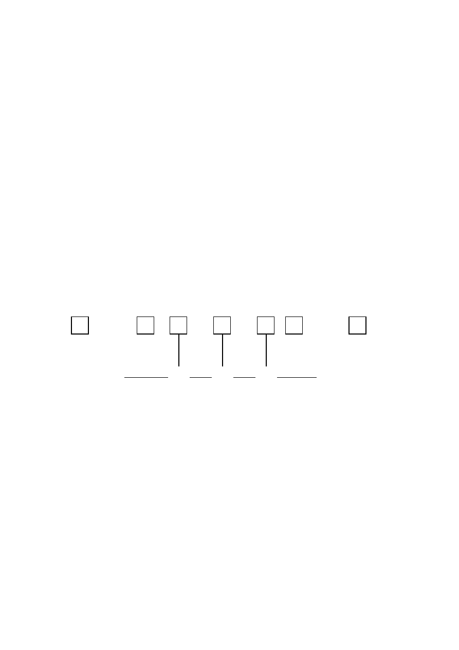
The model just described is displayed in Figure 4. We followed the standard con-
vention of denoting observed variables by squares and latent variables by circles.
The arrow between two latent variables represents transition process. The arrows
between the latent variables and the observed variables indicate the measurement
model (by means of conditional response probabilities).

½¼

¾»

00|96

½¼

¾»

Figure 3:

Path diagram that illustrates a two-indicator latent Markov model

for two waves.

Table 4 displays the estimated parameters of the two-indicator latent Markov

model with two states: "Poor" and "Non-poor" and Table 5 the same analysis for
quintiles.

We assumed that the response matrices are time invariant (R

= R

and R

= R

), i.e. the measurement error for both years is the same.

The first column displays the starting distribution, while the second column

displays the transitions between poverty states. The initial probabilities δ, show
that over 8 per cent are found to be in the poor class. This value exceeds both

In our analysis we assumed that the latent variables have the same number of classes as the

observed the categories.

For computations the program package PANMARK (Pol et al., 1998) has been used. The

estimates are ML and were obtained using the EM-algorithm.

Table 4:

Estimates of the two-indicator latent Markov model for the states "Poor"

and "Non-poor". Time interval: 1996 to 2000.

Latent states

Transitions in percent

Poverty state Start

Poor

Not poor

8.20

70.04

29.95

Poor

(1.5)

(1.1)

(1.0)

91.79

3.06

96.93

Not Poor

(1.5)

(1.4)

Response matrices R

latent states

observed states

42.00

58.00

Poor

(5.7)

0.03

99.96

Not Poor

(0.5)

47.12

52.88

Poor

(5.6)

Survey

6.86

93.14

Not Poor

(0.6)

Response matrix

Survey|Register=I

35.95

64.04

Poor

(2.0)

7.47

92.53

Not Poor

(0.3)

Standard Errors in Parenthesis

manifest measurements. The latent transitions probabilities show that the proba-
bility out of poverty is about 30 per cent. This is less than halved if we change
from the observed (Table 2) to the latent level (Table 4). The response probabili-
ties show that both incomes are bad indicators of the state "poor" (58 per cent of
those who are classified as poor in the "true" income are according to the regis-
ter income and 53 per cent according to the survey income observed not to be in
poverty). On the other hand the register income is perfect indicator of the state
non-poor whereas the survey income gives in 7 per cent the wrong indication of
the state non-poor. At the bottom of Table 4 survey response probabilities condi-
tioned on Register income=True income are displayed. This condition is achieved
by setting the register response matrices to be the identity matrix, i.e. R

= I. In

this case the survey response probabilities return the percentage of mismatches of
poverty states. In 64 percent of the cases where the person is poor with respect to
the register income he or she is not poor according to the survey income. These

Table 5:

Estimates of the two-indicator latent Markov model for Quintiles. Time

interval: 1996 to 2000.

Transition matrix:True

Response matrix:Survey|Register=I

Quintiles 1

73.50 14.80 9.30

2.40

0.00

42.50 36.60 10.30 5.60

5.00

(3.6)

(3.3)

(2.2)

(1.0)

(*)

(1.0)

(0.6)

(0.5)

(0.4)

13.60 59.70 22.30 5.40

0.00

19.70 30.60 30.70 13.40 5.60

(4.3)

(5.6)

(5.7)

(2.4)

(*)

(0.8)

(0.9)

(0.7)

(0.4)

4.50

16.40 57.90 13.80 7.40

14.30 15.20 32.10 29.50 8.90

(1.7)

(2.5)

(3.1)

(2.7)

(1.6)

(0.7)

(0.9)

(0.6)

8.70

0.00

16.30 62.40 13.70 12.10 10.20 14.60 37.70 25.30

(1.5)

(*)

(3.4)

(4.8)

(3.1)

(0.7)

(0.6)

(0.7)

(1.0)

(0.9)

2.90

2.60

2.80

18.00 73.70 10.00 9.00

7.70

17.70 55.60

(1.0)

(0.9)

(1.5)

(3.4)

(3.3)

(0.6)

(0.5)

(0.8)

(1.0)

Response matrix:Register

Response matrix:Survey

Quintiles 1

61.50 23.20 8.50

4.00

2.70

54.60 36.30 2.70

4.50

2.90

(2.0)

(2.1)

(1.1)

(0.7)

(0.5)

(2.8)

(1.5)

(1.7)

(0.7)

(0.8)

26.30 68.20 2.10

0.20

3.20

4.70

38.50 44.50 9.60

3.60

(5.0)

(5.6)

(5.9)

(2.0)

(0.8)

(3.5)

(3.1)

(3.9)

(1.8)

(1.4)

0.00

14.60 67.80 16.60 0.00

9.30

12.60 38.40 33.30 6.40

(*)

(3.2)

(3.4)

(2.7)

(*)

(1.1)

(1.3)

(1.9)

(0.8)

2.60

3.90

5.60

72.50 15.50 10.20 8.20

9.50

41.70 30.40

(1.1)

(1.4)

(2.9)

(4.0)

(3.1)

(1.0)

(0.8)

(1.2)

(1.7)

(2.0)

1.60

0.20

2.90

3.80

91.50 8.20

7.20

6.30

14.10 64.30

(0.8)

(0.5)

(0.9)

(2.6)

(3.0)

(0.8)

(0.7)

(1.3)

(1.7)

Standard Errors in Parenthesis

*) Parameter values bounded to 0 during the estimation

mismatches between the two income measurements are responsible for the much
higher stability at the latent level.

Turning to the results for quintiles in Table 5, we see that the stability at the la-

tent level (left above panel) is almost twice of what we observed on manifest level
for both measurements in Table 3. This is a consequence of the large percentage
where two income measurements do not lead to the same quintile position, indi-
cated by the right above panel in Table 5. Here the register measurement is taken
as the true state i.e. R

= I and consequently the response matrix R

returns the

percentage of mismatches of quintile positions. For each quintile position accord-
ing to the register, about 60 per cent observations have a different survey-quintile
position. In contrast to the results of the latent Markov model for two poverty
states where we took both measurements in the same way as indicators of the true

income, the register indicator here is a more reliable measurement of the true in-
come. This is indicated by the two panels at the bottom of Table 5. Except for the
lowest quintile, the reliability of the register measurement is almost 30 per cent
higher than the reliability of the survey measurement.

The LR value for above estimated LMM with two poverty states is LR=54

with df=9, while the LR value for LMM with quintile states results in LR=2131
with df=560.

Up to this point we only used the data from the waves 1996 and 2000 for both

incomes for our analysis not taking into account the fact that also the data for the
waves in between for register income are available. Taking this into account we
specified and estimated following 5-waves model.

P r(P

= i

, P

= i

, P

= j, P

= k, P

= l, P

= m

, P

= m

) =

a=1

b=1

c=1

d=1

e=1

97|96

b|a

j|b

98|97

c|b

k|c

99|98

d|c

l|d

00|99

e|d

(2)

The graphical representation of this model is given in Figure 4.

½¼

¾»

97|96

½¼

¾»

98|97

½¼

¾»

99|98

½¼

¾»

00|99

½¼

¾»

Figure 4:

Path diagram that illustrates a latent Markov model for five waves.

Table 6 below, displayed the estimated parameters of 5-wave LMM with two

states: "Poor" and "Non-poor". As in the previous case we have restricted the
response matrices to be stable over time. The first column returns the results if
both measurements are taken in the same way as indicators for the true state. In
the second column are results when we restricted register response matrix to be
the identity matrix, i.e. Register income=True income.
Both models show a decreasing trend to slip into poverty. However, for the risk
to stay in poverty the models give different answers. Here the register shows a
trend that this risk increases over the 5 waves, while the full latent model gives the
impression of a time–stable risk which is much higher as indicated by the register
income. So both models have quite different implications.

Table 6:

Estimates of the 5 waves latent Markov model. Time interval: 1996 to 2000.

4.59

95.40

3.91

96.08

Start

(0.4)

(0.3)

Transitions

81.01

18.98

39.44

60.55

96 to 97

(4.9)

(3.3)

3.20

96.78

4.29

95.70

(0.4)

(0.3)

79.37

20.62

53.16

46.83

(3.9)

(2.8)

1.74

98.25

3.14

96.85

97 to 98

(0.3)

(0.2)

78.59

21.48

60.66

39.33

(3.4)

(2.7)

2.06

97.93

3.09

96.90

98 to 99

(0.3)

(0.2)

84.03

15.96

59.06

40.93

(3.7)

(2.6)

1.23

98.76

2.68

97.31

99 to 00

(0.4)

(0.2)

Response matrices

73.49

26.50

100

(2.4)

0.87

99.12

100

(0.1)

45.07

54.92

35.95

64.04

(2.4)

(2.0)

6.62

93.37

7.46

92.53

Survey

(0.3)

Standard Errors in Parenthesis

Parameters values of 0 and 100 are fixed by definition

With respect to the response matrices which are displayed at the bottom of Ta-

ble 4 the survey income is a fairly bad indicator of the state ”poor”. If the survey
and the register are taken as imprecise measurements of the true income state, the
survey gives in 50 percent a mis-indication of poverty. This is twice as high as
for the register measurement. If the register is taken as true we see that this is not
indicated by the survey income in 2/3 of the cases. It is this small overlap of equal

states that forces the LMM to regard the majority of changes as measurement er-
rors resulting in these high stabilities on the latent level.
Turning to the results for quintiles in Table 5, we see that the stability at the latent
level (left above panel) is almost twice as what we observed on manifest level
for both measurements in Table 3. This is a consequence of the large percentage
where two income measurements do not lead to the same quintile position, indi-
cated by the right above panel in Table 5. Here the register measurement is taken
as the true state i.e. R

= I and consequently the response matrix R

returns the

percentage of mismatches of quintile positions. For each quintile position accord-
ing to the register, about 60 per cent observations have a different survey-quintile
position.
The LR test statistics for the five waves latent Markov model with two states
amounted to 480 (df=114) for full (when both measurements are taken in the
same way as indicators for the true income) and 686 (df=116) for register (when
register income equals true income) model. The poor fit of the models may be
due to the fact that we considered the Markov chain to be of first order not taking
into account the fact that the transition probabilities may not only depend on the
poverty state at time t but also on the poverty state at time t-1 (second-order) or
also at time t-2 (third-order). The second reason for the poor fit of the models may
be due to the assumption of population homogeneity. Instead the population may
be heterogenous with two or more chains, each of which has its own dynamics.

3.3

A Latent mixed Markov model for transitions between in-
come states

Since in the last section we have assumed a population homogeneity (only one
chain of latent transitions), we relax this assumption in this section imposing a la-
tent mixed Markov model, see Langeheine (1990). This model emerges from the
combination of mixed Markov chains and models that can incorporate measure-
ment error (LMM). The chains are latent and the sizes of the chains are estimated
from the model. The general latent mixed Markov model for 5-waves (two indica-
tors for waves 1996 and 2000 and one indicator for waves 1997, 1998 and 1999)
can be written as

P r(P

= i

, P

= i

, P

= j, P

= k, P

= l, P

= m

, P

= m

) =

s=1

a=1

b=1

c=1

d=1

e=1

a|s

|as

97|96

b|as

j|bs

98|97

c|bs

k|cs

99|98

d|cs

l|ds

00|99

e|ds

|es

(3)

where π

are the proportion of S latent chain (proportion of the population behav-

ing according to latent Markov chain s). The interpretation of other parameters is

the same as in the above models except the fact that within each chain, the chain
variable is added as a conditioning variable to the parameters. The problem when
fitting this model is that the model wouldn’t be identified unless some parameter
restrictions are imposed. Because of this problems we fitted the following two-
chain (S=2) latent Markov model: There is a latent change and a response error
for the first chain (mover chain) and no latent change and no response error for
the second chain (stayers chain). The assumption that the stayers do not make
response errors is plausible because it is easy to produce the correct answer if
one’s position is stable. It is also practical because of the parsimony of the model
parameters (this model adds only two parameters to the one-chain latent Markov
model).
For the mover chain we restricted response probabilities to be time invariant i.e.,
R

= R

and R

= R

Furthermore, we left transitions matrices to be free between the time points.
For the stayer chain we considered following specification:
R

= R

= I

97|96

b|a

= τ

98|97

c|b

= τ

99|98

d|c

= τ

00|99

e|d

= I

where "I" denotes the Identity matrix.
Table 7, below presents the estimated parameter values from the model. In Table 7
the first column presents the chain proportion of movers, their initial distribution,
transitions between subsequent states for the movers and their response probabil-
ities, whereas the second column presents the same values for the stayers. From
Table 7 we see that the population is almost equally divided into movers and stay-
ers. The initial distribution for the stayers shows that 98 per cent of these belong
to Non-Poor class.

By multiplying the chain proportion of stayers with their initial distribution,

we get the proportion of the population that are either never in poverty or always
in poverty. Consequently 51 per cent of the population will never be in poverty
and there is only 0.7 per cent of the population who will always be observed
as poor. The latent transition probabilities for the movers are similar to those
estimated for the 5-waves register latent Markov model, there is a decreasing trend
of slipping into poverty and an increasing trend of staying in poverty over the time.
The response probabilities show that the register measurement is almost perfect
indicator for both latent classes, while survey measurement gives in 60 per cent
mis-indication of poverty and in 16 per cent mis-indication of non-poverty.
The LR statistic for this model resulted in 370 (df=112).

Table 7:

Estimates of 5-waves latent mixed Markov model. Time interval: 1996 to

2000.

Chain

Movers

Stayers

47.87

52.13

Chain proportion

(2.4)

7.12

92.88

1.26

98.74

Start

(0.8)

(0.1)

Transitions

59.75

40.24

100

96 to 97

(6.9)

(fixed)

7.81

92.19

100

(1.0)

(fixed)

69.66

30.34

100

97 to 98

(4.8)

(fixed)

4.87

95.13

100

(0.8)

(fixed)

71.09

28.91

100

98 to 99

(3.5)

(fixed)

4.82

95.17

100

(0.7)

(fixed)

73.60

26.40

100

99 to 00

(4.2)

(fixed)

3.70

96.30

100

(0.8)

(fixed)

Response matrices

87.21

12.79

100

(2.9)

(fixed)

1.93

98.07

100

(0.4)

(fixed)

38.59

61.41

100

(2.7)

(fixed)

16.13

83.87

100

Survey

(1.1)

(fixed)

Standard Errors in Parenthesis

Parameter values of 0 and 100 fixed by definition

3.4

Stability and Change

The above analysis of the different Markov models has shown that the change
between specific income states is overestimated and consequently the stability un-

derestimated if the problem of measurement error is neglected. The latent Markov
models offer the possibility to break down the proportions of observed stability
and change into true and error components. For this reason it is necessary to cal-
culate the total proportion of stability and change. The total proportion of stability
over 5 time points (from 1996 to 2000) can be expressed by:

T OS =

a=1

97|96

b|a

98|97

c|b

99|98

d|c

00|99

e|d

(e=d=c=b=a)

(4)

This is simply the number of individuals who do not change their initial state
throughout the observation period, expressed as a proportion of the total sample.
Consequently, total change (TOC) is equal to TOC=1-TOS. Now, taking into ac-
count the measurement error we can separate both TOS and TOC into a true part
and an error part by conceiving the response probabilities. The true stability (TRS)
is thus given by:

T RS =

a=1

b=1

c=1

d=1

e=1

97|96

b|a

98|97

c|b

99|98

d|c

00|99

e|d

)

= a, i

= a, j=b, k=c, l=d, m

= e, m

= e and e=d=c=b=a)

(5)

This can be thought of as that proportion of the true stability which is observed.
The error proportion of total stability (ERS) is equal to ERS=TOS-TRS. The same
consideration can be made for the total change. Here true change (TRC) is the
proportion of latent change which is observed as such:

T RC =

a=1

b=1

c=1

d=1

e=1

97|96

b|a

j|b

98|97

c|b

k|c

99|98

d|c

l|d

00|99

e|d

= a, i

= a, j=b, k=c, l=d, m

= e, m

= e, not e=d=c=b=a) (6)

The error proportion of change (ERC) is equal to ERC=TOC-TRC.
Table 8 gives estimated proportions of 5-waves latent and mixed latent Markov
models for the two income states and also respective proportions in the data (Col-
umn "Data") where the two cells with response patterns 1111111 and 2222222

We have done this analysis only for five waves models.

indicate stability and the rest corresponds to change.
In Table 8 for the mixed latent Markov model (MLM) we also displayed the Per-
fect Stability which is defined as a proportion of the sample in the stayer latent
class. From Table 8 we see that according to three under consideration taken
models proportions of true stability are 74.89%, 71.93% and 74.99% (including
52.13% perfectly stables in the last case). This makes evident that the observed
data understate true stability and overstate change. Expressed as a percentage of
observed change, we see that according to LM 58% of observed change is error,
according to LM(R=I) 36% and according to MLM 54%. These results support
the findings of the last sections, namely that most of the change is due to measure-
ment error.

Table 8:

Estimated proportions of stability and change

Model

Data

LM(R=I)

MLM

Perf.Stab.

52.13

TOS

75.35

89.68

84.26

36.48

TRS

74.89

71.93

22.86

ERS

14.79

12.33

13.62

TOC

24.65

10.32

15.74

11.39

TRC

2.82

8.41

3.64

ERC

7.50

7.33

7.75

Total error

22.29

19.66

21.37

LM=latent Markov model (Table 6)

LM(R=I)=LM when Register income=True income (Table 6)

MLM=mixed latent Markov model (Table 9)

Panel attrition

In this section we study the impact of attrition on the estimation of Markov chain
models for transitions between income states. Panel attrition affects the sample
composition and has therefore the potential to bias the estimates.

The reasons for

the panel attrition may have different sources:

• The target person may refuse to cooperate.

• The target person is not able to respond (e.g., due to illness).

• Failure in tracing mobile respondents.

• The agency collecting the data failed to get into contact with the target per-

son.

To obtain the estimates of transition probabilities for attriters, respondents and

respondents and attriters we split our sample in 1996 into samples of attriters and
respondents, according to the response behavior in 2000. Since the register also
provides data for the attriters we have for the group of the respondents for both
years both income measurements and for the group of the attriters for the year
1996 both income measurements and for the year 2000 only register measure-
ment. The graphical representation of the model for the attriters is given in the
Figure 5, since the graphical representation of the respondents model equals the
graphical representation in the Figure 3.

½¼

¾»

00|96

½¼

¾»

Figure 5:

Path diagram that illustrates a two waves latent Markov model for

the attriters.

The transition matrix between the latent states is of the main interest here and

we want to know whether its estimation is affected by attrition. The estimation of
the full sample uses both samples, the respondents sample and the attriter sample.
Here we have to restrict the transition matrix for the respondents, τ

N A

, to be equal

See Sisto, [2003].

See Rendtel, [2002].

to the transition matrix of the attriters, τ

. This restriction leads to the estimator

based on the full sample, τ

ALL

. However, the response matrices for the two groups

are allowed to differ. The restricted sample uses only the information from the
respondent sample. In this case τ

N A

is estimated freely without restriction to the

attriter sample. Finally we are interested in the transition matrix τ

based on the

attriter sample alone. For these purposes we estimated the following two groups
latent Markov model.

P r(P

= i

, P

= i

, P

= j

, P

= j

)

= γ

a=1

b=1

a|h

|ah

00|96

b|ah

|bh

(7)

where γ

is the proportion of population that belongs to subpopulation h (here

h=2).
Table 9 displays the results for the switches between the poor and the non-poor
states. The above panel of Table 9 returns the results when also the register is
regarded as an imperfect measurement for the true state. The panel underneath
treats the register income as the true income. In both cases the probability to stay
poor is higher for the attriters than for the non-attriters. Also the risk to slip into
poverty is much higher for the attriters than for the non-attriters. Thus the risk of
the attriters is less favorable than the risk of the non-attriters.

Table 9: Estimated transition probabilities between poverty status (1996 to
2000). τ

N A

= τ

: Estimation based on the full sample, τ

N A

: Estimation based on

the respondent sample, τ

: Estimation based on the attriters

= τ

N A

1996

poor

not poor

poor

not poor

poor

not poor

full model: register + survey income = true income

83.73

16.27

88.44

11.56

100

0.00

Poor

(5.8)

(6.9)

(1.7)

(fixed)

14.92

85.09

10.86

89.14

25.97

74.03

Not Poor

(1.6)

(6.9)

(1.7)

(5.9)

33.23

66.77

32.26

67.74

36.05

63.95

Poor

(2.6)

(3.0)

(0.3)

7.32

92.68

5.55

94.45

13.22

86.78

Not Poor

(0.3)

(5.2)

(0.8)

Standard Errors in Parenthesis

Table 10:

Estimated transition probabilities between income quintiles

(1996 to 2000). τ

N A

= τ

: Estimation based on the full sample, τ

N A

: Esti-

mation based on the respondent sample, τ

: Estimation based on the attriters

Quintile

in 1996

Quintile in 2000

N A

= τ

71.39 17.30 9.25

2.06

0.00

54.64 24.10 12.59 6.29

3.36

(2.7)

(3.1)

(1.9)

(0.8)

(*)

(1.2)

(1.0)

(0.8)

(0.6)

(0.9)

25.06 56.05 13.79 6.10

0.00

24.72 37.08 21.29 13.11 3.81

(2.7)

(4.9)

(4.7)

(2.1)

(*)

(1.1)

(1.2)

(1.0)

(0.8)

(0.5)

3.48

15.56 58.22 15.29 7.45

14.58 21.04 34.97 18.99 10.42

(1.8)

(2.9)

(3.5)

(2.9)

(1.5)

(0.9)

(1.0)

(1.2)

(1.0)

(0.8)

9.66

0.00

20.33 54.58 15.43 10.41 9.64

21.21 37.27 21.46

(1.5)

(*)

(3.5)

(4.4)

(2.7)

(0.8)

(0.7)

(1.0)

(1.2)

(1.0)

4.26

2.70

2.41

17.67 72.95 7.32

5.68

8.52

19.00 59.47

(1.0)

(1.5)

(2.9)

(3.0)

(0.7)

(0.6)

(0.7)

(1.0)

(1.2)

N A

73.68 16.02 6.95

3.35

0.00

51.67 24.25 13.50 7.18

3.50

(2.9)

(2.0)

(3.0)

(1.4)

(*)

(1.4)

(1.2)

(1.0)

(0.7)

(0.5)

6.91

61.93 12.37 18.79 0.00

23.86 40.14 22.27 13.73 0.00

(2.4)

(3.2)

(3.7)

(2.9)

(*)

(1.3)

(1.5)

(1.2)

(1.0)

(*)

0.00

1.42

98.48 0.00

0.09

11.98 20.38 36.44 19.97 11.28

(*)

(4.5)

(6.0)

(*)

(2.8)

(0.9)

(1.2)

(1.4)

(1.2)

(0.9)

0.55

8.31

22.14 55.29 13.71 8.52

8.19

21.34 39.87 22.08

(1.9)

(2.1)

(4.1)

(3.4)

(2.0)

(0.8)

(1.2)

(1.4)

(1.2)

0.32

0.28

13.08 11.93 72.49 5.96

4.72

8.69

20.20 60.53

(1.3)

(1.0)

(3.7)

(2.4)

(3.3)

(0.7)

(0.6)

(0.8)

(1.2)

(1.4)

83.87 15.47 0.00

0.00

0.60

64.75 17.80 10.18 4.22

3.06

(5.9)

(6.2)

(4.4)

(*)

(1.4)

(2.3)

(1.9)

(1.5)

(1.0)

(0.8)

33.96 44.93 9.25

11.86 0.00

32.28 32.57 23.43 11.71 0.00

(4.7)

(5.8)

(6.7)

(4.5)

(*)

(2.5)

(2.3)

(1.7)

(*)

6.16

33.57 60.07 0.00

0.00

24.14 20.11 31.32 16.38 8.05

(8.9)

(18.1)

(22.0)

(20.5)

(*)

(2.3)

(2.1)

(2.5)

(2.0)

(1.5)

18.74 2.49

19.43 39.04 20.20 17.88 10.30 21.82 29.77 20.33

(3.8)

(5.4)

(9.3)

(6.6)

(3.8)

(2.1)

(1.7)

(2.3)

(2.5)

(2.2)

12.69 0.000 0.00

21.72 65.59 12.05 6.03

8.49

15.62 57.81

(2.5)

(*)

(3.1)

(3.3)

(1.7)

(1.2)

(1.5)

(1.9)

(2.6)

Standard Errors in Parenthesis

*) Parameter values bounded to 0 during the estimation

A similar finding holds for the quintiles in Table 10. Also here the risk to

switch to or to stay in the lowest quintile is much higher for the attriters than for
the non-attriters. Besides, the attriters are in general more unstable. The same
finding holds also if we take the register income to be the true income (heading
"Register=True" in Table 10).

The general pattern is that less favorable income profiles are more frequent for

attriters. This is a finding which is in line with events like a divorce or getting
unemployed. However, the bias induced by these trends is small.
To asses the attrition bias, we carry out the Hausman-test to test whether the dif-
ference between the estimates using only the information of respondents (τ

N A

)

and the estimates using the information of attriters as well as respondents (τ

ALL

)

is significant. The estimate of the bias is

ˆb(τ) = ˆτ

N A

− ˆ

ALL

The hypothesis b(τ ) = 0 is tested against the alternative b(τ ) 6= 0 making use of
the asymptotic result that the covariance matrix of the difference Σ

dif f

between

a consistent estimator under the null-hypothesis (τ

N A

) and an efficient estimator

(τ

ALL

) is given by their difference:

dif f

= Σ

− Σ

ALL

(8)

The Hausman-test statistic is then calculated as

t = (ˆ

N A

− ˆ

ALL

)

−1

dif f

(ˆ

N A

− ˆ

ALL

) ∼ χ

Table 11 contains the Hausman-tests.

Table 11:

Results of the Hausman-test.

Model

chi-square

p-value

Full model

with two states

1.5417

0.4626

with two states

0.3736

0.8296

Full model

with Quintiles

14.8087

0.7347

In the case of the full model with quintiles the standard deviation of some ˆ

N A

parameters was estimated to be smaller than standard deviation of ˆ

ALL

parame-

ters leading to a non-applicability of the Hausman-test. This case is marked with
(*) in Table 11. According to the Hausman-test we get no significance for the
rejection of the Null-hypothesis that all transition elements are equal.

Conclusion

The objective of this work was to find out how reliable the two income measure-
ments are and to what extent measurement error and panel attrition affects the
estimates of the income mobility. With respect to these questions we have fitted
several latent Markov models with survey and register income as indicators for the
true income. Our results show that not correcting for measurement error influence
conclusions we might draw about income mobility. Thus, much of the observed
movement into and out of poverty is caused by error in the measurement of in-
come. The reason for this is that the measurement error is modelled as change.
We also found that the poor position is rather badly identified, and much less ac-
curately measured than the non-poor.
With respect to the reliability of the two measurements we found that the income
state measured by the survey income is less reliable than the state measured by
the register income. The survey information also suggests systematically higher
instability as compared to the register information.
With respect to the panel attrition effects our analysis revealed that there is a mild
attrition bias on the estimates of the income mobility. The attriters are more fre-
quent among persons who stay in poverty or who switch to lower income posi-
tions. The transition probabilities estimated for respondents show slightly less
mobility than transition probabilities estimated for the full sample.
The results presented in this work demonstrate that the measurement error has a
much higher impact on the income mobility than the attrition bias and the impor-
tance of taking the existence of measurement error in studies of income dynamics
into account.

References

[1] Bishop, Yvonne/Finberg, Stephen/Holland, Paul (1995): Discrete Multivari-

ate Analysis, MIT Press, Cambridge.

[2] Breen, Richard and Moisio, Paul (2003): Poverty Dynamics Corrected for

Measurement Error, Working Papers of the Institute for Social and Economic
Research, paper 2003-17. Colchester, University of Essex.

[3] Dempster, A.P./Laird, N.M./Rubin, D.B. (1977): Maximum Likelihood from

Incomplete Data via the EM Algorithm, Journal of the Royal Statistical So-
ciety, Series B, 39, pp. 1-38.

[4] Efron, B. and Tibshirani, R.J. (1993): An Introduction to the Bootstrap, New

York.

[5] Eurostat (2000): ECHP Data Quality - Second Report.

[6] Langeheine, Rolf and van de Pol, Frank (1990): A Unifying Framework

for Markov Modelling in Discrete Space and Discrete Time, Sociological
Methods and Research, 18, pp. 416-441.

[7] Langeheine, Rolf and van de Pol, Frank (1994): Discrete-Time Mixed

Markov Latent Class Models, in: A. Dale/R. Davies (eds.): Analyzing Social
and Political Change: A Case Book of Methods, London pp. 170-197.

[8] Neukirch, Thomas (2002): Nonignorable Attrition and Selctivity Biases in

the Finnish Subsample of the ECHP - An empirical Study Using Additional
Register Information, CHINTEX Working Paper #5.

[9] Nordberg, L./Pentillä, I./Sandström, S. (2000): A Sutdy on the Effects of

Using Interview versus Register Data in Income Distribution Analysis with
an Application to the Finnish ECHP-Survey in 1996, CHINTEX Working
Paper #8.

[10] Peracchi, Franco (2002): The European Community Household Panel: A

Review, Empirical Economics, Vol.27, pp. 63-90.

[11] Rendtel, Ulrich (2002): Attrition in Household Panels: A Survey, CHINTEX

Working Paper #4.

[12] Rendtel, Ulrich/Hanisch, Jens/Nordberg, Leif (2003): Report on the Work

Package: "Quality of Income Data", CHINTEX Working Paper.

[13] Rendtel, Ulrich/Langeheine, Rolf/Berntsen, Roland (1998): The Estimation

of Poverty Dynamics Using Different Measurements of Household Income,
Review of Income and Wealth, 44, pp. 81-98.

[14] Silverman, B. (1986): Density Estimation for Statistics and Data Analysis,

Chapman and Hill, London.

[15] Sisto, Johanna (2003): Attrition Effects on the Design Based Estimates of

Disposable Household Income, CHINTEX Working Paper #6.

[16] van de Pol, Frank and de Leeuw, Jan (1986): A Latent Markov Model to

Correct for Measurement Error, Sociological Methods and Research, 15, pp.
118-141.

[17] van de Pol, Frank/Langeheine, Rolf/de Jong, Wil (1998): PANMARK 3

User’s Manual: Panel Analysis Using Markov Chains, Netherlands Central
Bureau of Statistics, Vorburg.

Wyszukiwarka

Podobne podstrony:
markov v1-streszczenie
duration analysis v1 artykul id Nieznany
markov v1 streszczenie
nieparametryczne v1 artykul
bayes v1 artykul
gmm v1 artykul a
markov v2 artykul
panele v1 artykul
gmm v1 artykul b
PO wyk07 v1
s10 v1
s7 4 v1
s9 3a v1
dodatkowy artykul 2
ARTYKUL

więcej podobnych podstron