Bayesian option pricing using asymmetric

GARCH models

Luc Bauwens

a,b,

*, Michel Lubrano

CORE, Voie du Roman Pays, 34, 1348 Louvain-La-Neuve, Belgium

Department of Economics, Universite´ Catholique de Louvain, Belgium

GREQAM-CNRS, Belgium

Accepted 23 November 2001

Abstract

This paper shows how one can compute option prices from a Bayesian inference viewpoint, using

a GARCH model for the dynamics of the volatility of the underlying asset. The proposed evaluation
of an option is the predictive expectation of its payoff function. The predictive distribution of this
function provides a natural metric, provided it is neutralised with respect to risk, for gauging the
predictive option price or other option evaluations. The proposed method is compared to the Black
and Scholes evaluation, in which a marginal mean volatility is plugged, but which does not provide a
natural metric. The methods are illustrated using symmetric, asymmetric and smooth transition
GARCH models with data on a stock index in Brussels.

D 2002 Elsevier Science B.V. All rights

reserved.

JEL classification: C11; C15; C22; G13
Keywords: Bayesian inference; GARCH; Option pricing; simulation

1. Introduction

The Black and Scholes (hereafter BS) formula for option pricing is a function of the

parameters of the diffusion process describing the dynamics of the underlying asset price.
The BS formula is derived for a geometric Brownian motion with a constant volatility
parameter r (corresponding to a hypothesis of homoskedasticity in an econometric model).

0927-5398/02/$ - see front matter

PII: S 0 9 2 7 - 5 3 9 8 ( 0 1 ) 0 0 0 5 8 - 5

Corresponding author. CORE, Voie du Roman Pays, 34, 1348 Louvain-La-Neuve, Belgium. Tel.: +32-10-

47-4336; fax: +32-10-47-4301.

E-mail address: bauwens@core.ucl.ac.be (L. Bauwens).

www.elsevier.com/locate/econbase

Journal of Empirical Finance 9 (2002) 321 – 342

In order to apply the BS formula, the econometrician has to estimate the parameter r of the
diffusion process. Hull and White (1987) studied option pricing in the case of stochastic
volatility, where r

follows an independent geometric Brownian motion. Provided the

increments of the volatility process are independent of the increments of the process
governing the asset price, they showed that options can be priced by averaging the BS
formula over the stochastic volatility, i.e. that there is no need to price the risk attached to
the stochastic volatility. Noh et al. (1994) predict the future mean volatility using a
generalised autoregressive conditional heteroskedasticity (GARCH) model on the past
returns and plug it in the BS formula.

They conclude that the GARCH estimated volatility

has more economic content than the volatility estimates obtained by inverting the BS
formula using observed past option prices.

When relaxing the hypothesis of constant volatility, it is very difficult, if not

impossible, to solve the partial differential equation that leads to the BS formula (see,
however, the restrictive case of Hull and White (1987) cited above and also the paper of
Heston and Nandi (2000)). One has to apply the risk-neutral pricing methodology of Cox
and Ross (1976), that is to say, for evaluating the price of a call option at time t with
maturity at time T > t, compute

¼ e

rðT tÞ

max

ðS

K; 0Þ

;

ð1Þ

where K is the exercise price, r the riskless interest rate and S

the predicted price of the

underlying asset at time T. This procedure requires to find an equivalent martingale
measure for the returns, which leaves the volatility unchanged (in a way to be precised
later) and for which the returns behave like a martingale. Duan (1995) derived the
equivalent martingale measure for the case where the returns follow a discrete GARCH
process with normal errors. Duan (1999) provides extensions to the case of leptokurtik
errors. Kallsen and Taqqu (1998) make the bridge to continuous time GARCH, while
Garcia and Renault (1997) compare option pricing and hedging when heteroskedasticity is
of the GARCH type or of the stochastic volatility type.

The object of this paper is to investigate the interesting features that the Bayesian

approach may bring in the risk-neutral methodology for option pricing. We have first to
select an econometric model that captures as best as possible the well-known stylised facts
of financial return series: volatility clustering

, strong kurtosis, and often in the case of

stocks, the leverage effect. We have basically the choice between two families of models.
The stochastic volatility model in discrete time is certainly the model that is the closest to
the continuous time diffusion processes considered in Hull and White (1987). Mahieu and
Schotman (1998) estimated various specifications of the stochastic volatility model and
applied directly the solution of Hull and White (1987) for option pricing. However, when
we introduce a leverage effect in this model, we allow for possible correlation between
volatility increments and the increments of the process and thus violate Hull and White’s

Note, however, that using the BS formula with an estimated r computed as the average volatility results in

mispricing because of Jensen’s inequality.

Volatility clustering of the returns induces a slowly decaying autocorrelation function of the squared returns,

starting at a rather small value (about 0.2, 0.3). See, e.g. Terasvirta (1996) and Pagan (1996).

L. Bauwens, M. Lubrano / Journal of Empirical Finance 9 (2002) 321–342

322

assumption. Moreover, Mahieu and Schotman concluded that the obtained estimates for
the volatility were very imprecise. The GARCH model, which is much simpler to estimate,
recovers thus all of its interest and we make it our baseline model.

Once risk neutralisation is taken into account, we have to simulate the chosen model in

a way that takes into account all the available information contained in the data. The
Bayesian viewpoint is particularly well suited for this requirement. The predictive density
is a natural by-product of inference that can be used for prediction as it represents the
density of future observations. The risk-neutral valuation requires the use of the predictive
expectation of the payoff function of the option given in Eq. (1), which we call the
predictive option price. We can even compute the predictive density of the payoff function.
In the classical framework, a point estimate of the option price can also be computed, but
the Bayesian approach delivers naturally a probability distribution. This distribution
integrates the uncertainty both over the parameter values of the underlying econometric
model (contained in the posterior distribution of the parameters) and over the future stock
price. Therefore, an interval estimate of any confidence level can be formed for an option
price. If an agent wants to buy (or sell) an option on the market, he can gauge the market
price of the option with the predictive distribution of the option price, e.g. he could decide
not to buy (sell) if the market price is too far in the right (left) tail of his predictive
distribution.

Let us define returns in discrete time

¼ ðS

Þ=S

ð2Þ

The baseline GARCH(1,1) model with Gaussian errors

¼ l

þ u

j I

ð0; h

¼ x þ au

2
t

þ bh

;

ð3Þ

where l

represents the conditional expectation of the returns, was used for instance by

Noh et al. (1994). This simple model does not succeed completely in reproducing the
stylised facts present in the data and consequently may give a wrong account of the
volatility persistence. The degree of persistence in the volatility process is important for
option pricing since a higher persistence results in a longer delay for the predictive
conditional variance to converge to its unconditional value. As shown in detail by
Terasvirta (1996), the introduction of Student errors improves greatly the possibility that
the GARCH(1,1) model reproduces the behaviour of data with a high empirical kurtosis. A
second possible improvement of GARCH models for stock returns consists in taking into

Duan (1995) considers in fact y

= Dlog(S

), which is the continuous time equivalent of y

=(S

)/S

The discrete time formulation leads to simpler results for risk neutralisation as one does not have to manipulate
lognormal distributions.

The parameters a, b and x are restricted to be positive. The starting value h

is treated as a known constant.

The {e

} sequence is conditionally independent. I

is the past information set.

L. Bauwens, M. Lubrano / Journal of Empirical Finance 9 (2002) 321–342

323

account the leverage effect, which is the negative correlation between current stock returns
and future volatility. In the model of Glosten et al. (1993), the conditional variance can
react asymmetrically to past squared shocks in the mean process, a stronger effect for
negative shocks than for positive ones corresponding to the leverage effect. Finally,
besides asymmetry, the news impact curve of the GARCH model may saturate for large
returns. Lubrano (2001) introduces a smooth transition GARCH model that combines both
asymmetry and saturation.

The paper is organised as follows. Section 2 presents in general terms the predictive

option pricing method and the option pricing rules. Section 3 introduces and discusses two
variants of the GARCH model that are used for an empirical application on an index of the
Brussels stock exchange. Section 4 provides the computational details on Bayesian option
pricing and illustrates the method on the empirical GARCH models developed in the
previous section. Section 5 concludes.

2. Predictive option pricing: principles

2.1. Introduction

The terminal payoff at time T of a European call option is given by

¼ maxðS

K; 0Þ:

ð4Þ

If we manage to find a risk-neutral equivalent martingale measure Q to the measure P of
the empirical process of the underlying security return, then an option can be priced as the
discounted expected value of its future terminal payoff. When the empirical process
follows a geometric Brownian motion, an analytical solution to this problem is provided
by the celebrated BS formula

¼ S

ðd

Þ Ke

rðT tÞ

ðd

rðT tÞ

ﬃﬃﬃﬃﬃﬃﬃﬃﬃﬃﬃ

þ 0:5r

ﬃﬃﬃﬃﬃﬃﬃﬃﬃﬃﬃ

rðT tÞ

ﬃﬃﬃﬃﬃﬃﬃﬃﬃﬃﬃ

0:5r

ﬃﬃﬃﬃﬃﬃﬃﬃﬃﬃﬃ

;

ð5Þ

where U(

) is the cumulative Gaussian distribution function, S

the observed price at time t

of the underlying security, and K the exercise price or strike. The arguments depend on the
volatility r, which is the standard deviation (per time unit) of the process of the return of
the underlying asset. Methods to estimate this parameter can be found for instance in
Campbell et al. (1997) as well as an extension for the case where the underlying price
follows a trending Ornstein – Uhlenbeck process.

L. Bauwens, M. Lubrano / Journal of Empirical Finance 9 (2002) 321–342

324

2.2. Stochastic volatility

In the case of stochastic volatility (r indexed by t), provided volatility is uncorrelated

with the security price (which excludes GARCH processes), one can follow Hull and
White (1987) and average the BS formula over future volatility in a Monte Carlo
simulation of N draws so as to obtain

¼1

ðS

;

K; r

Þ;

ð6Þ

where

¼tþ1

j;i

ð7Þ

The main advantage of this approach is that we do not have to predict the future price S

the underlying asset. We have only to predict future volatility under measure P.
Consequently, there is no need to find an equivalent risk-neutral process to the data
generating process. However, this approach is limited in its application as, first, it
precludes any correlation between the price of the underlying asset and the volatility
(leverage effect) and, second, it cannot price the risk attached to stochastic volatility.

2.3. GARCH option pricing and risk neutralisation

Duan (1995) provides a general method for option pricing in the case of GARCH

processes. Risk neutralisation should leave the variance unchanged and should transform
the conditional expectation so that the discounted expected price of the underlying asset
follows a martingale. In GARCH processes, it is not possible to find a risk-neutralisation
procedure that leaves unchanged the marginal variance of the process or the conditional
variance beyond one period. Duan (1995) introduces the local risk-neutral valuation
relationship, which leaves unchanged the one period ahead conditional variance and
implies that the expected future return is equal to the risk-free interest rate r. Adapted to
discrete time, this means that

ðS

Þ=S

¼ r:

ð8Þ

The econometric model (3) specifies the empirical distribution of y

defined in Eq. (2),

conditionally on the past. The pricing measure Q shifts the error term u

so that the

conditional expectation of y

becomes equal to r. The new error term is v

= u

+ l

r and

we have

¼ r þ v

j I

ð0; h

¼ x þ aðv

þ rÞ

þ bh

ð9Þ

L. Bauwens, M. Lubrano / Journal of Empirical Finance 9 (2002) 321–342

325

The functional form of the conditional variance remains unchanged. However, h

is no

longer governed by a v

variable as under measure P but by a noncentral v

. This type of

shifting can be applied to many other GARCH processes, in particular those reviewed in
the introduction, which take into account asymmetry, leverage effect and saturation.

Duan (1995) used the GARCH-M model of Engle et al. (1987), which implies that

¼ l þ k

ﬃﬃﬃﬃ

(one must note that the GARCH-M model combines nicely with the

properties of the lognormal distribution). This model, which may find some justification in
the financial literature, generally has not a very good fit and provides poor estimates for k.
As noted for instance by Campbell et al. (1997, Chap. 2), financial series such as stock
indexes often present positive autocorrelation of the returns. Positive autocorrelation may
be due to various phenomena such as infrequent and nonsynchronous trading of individual
stocks entering the index, but it also may be due to the risk premium attached to
nonconstant volatility. Consequently, the baseline GARCH model with normal errors we
selected is

¼ l þ qy

þ u

j I

ð0; h

¼ x þ au

2
t

þ bh

ð10Þ

We follow the same approach as Hafner and Herwartz (2001) who found on German
securities that incorporating qy

in the conditional expectation gave a higher likelihood

value than incorporating kh

. The variance of y

is as usual equal to x/(1

a b) and the

stationarity condition is given by a + b < 1. For the risk-neutralised process, we show in
Appendix A that the variance is

Var

ðy

Þ ¼

þ a½ð1 qÞr l

að1 þ q

Þ b

ð11Þ

The process is stationary if a(1 + q

) + b < 1. Consequently, risk neutralisation increases the

marginal variance of y, fragilises the stationarity condition and increases volatility
persistence as the predictive variance will take a longer time to converge to its limiting
value given in Eq. (11).

2.4. Predictive option pricing

The predictive density of the terminal payoff P

under measure Q is defined by

ðP

j yÞ ¼

ðP

j h; yÞuðh j yÞdh;

ð12Þ

where u(h

jy) is the posterior density of the parameters of the econometric model (10),

( P

jh, y) is the density of a future payoff after translation of the error term, and y is the

sample of returns used for estimation. The predictive density (12) gives us all the
information we need to compute the predictive option price, which is just the predictive
expectation of P

multiplied by (1 + r)

(T t)

as we are in discrete time for discounting.

L. Bauwens, M. Lubrano / Journal of Empirical Finance 9 (2002) 321–342

326

The Bayesian approach provides a complete density so that a measure of uncertainty can
be attached to the option price by computing a confidence interval.

The predictive density of either P

, S

or y

is not straightforward to compute in a

GARCH model. Details can be found in Bauwens et al. (1999, Chap. 7) for the usual
GARCH model. When T = t + 1, which means that ns (the number of predictions ahead) is
equal to one, the conditional density of a future return y

under measure Q is a normal

density given by

ðy

j h; y

Þ ¼ f

r; x

þ a½ y

l qy

þ r

þ bh

ð13Þ

Conditionally on h, all the parameters of this distribution are known as y

and h

are

observed or already computed. When ns>1, the complete predictive is obtained by the
multiple integral

ð y

j y

Þ ¼

ð y

j h; y

Þf

ð y

j h; y

Þ : : :

ð y

þ1

j h; y

Þuðh j yÞdy

: : : dy

þ1

dh:

ð14Þ

We have to integrate h as in Eq. (12), but also y

t + 1

,. . ., y

, which are unobserved, but

can be simulated sequentially. The dimension of the integration over future y

t + j

is thus

1. Each element in Eq. (14) is a normal density with mean r and variance h

t + j

, but the

resulting density in the inner integral is not of a known form. We propose in Section 4 a
simulation algorithm that draws random numbers in the predictive density (14) and is
inspired from Geweke (1989). Once a simulated sequence y

(i = t + 1,. . ., T) is obtained, it

is transformed into a draw from the predictive density of P

through the following

transformation

¼ S

¼tþ1

ð1 þ y

¼ maxðS

K; 0Þ:

ð15Þ

The predictive option price is defined as the discounted expectation of P

. When we have

obtained N draws P

( j = 1,. . ., N) of P

, the predictive option price can be approximated

by the empirical mean

ð1 þ rÞ

ðT tÞ

¼1

ð16Þ

With the same draws, we can estimate the complete predictive density of P

using a

nonparametric approach.

The empirical mean (16) converges to its population value if the empirical process is

stationary. As we are in a Bayesian framework, the stationarity condition may be verified
at the posterior mean of h, but not necessarily for every point drawn from the posterior

L. Bauwens, M. Lubrano / Journal of Empirical Finance 9 (2002) 321–342

327

density. The points for which the stationarity condition is not met have to be rejected for
the predictive evaluation

As Eq. (16) is a Monte Carlo estimator, we would like to qualify its precision. Let us

define the empirical standard deviation of C

¼ ð1 þ rÞ

ðT tÞ

ﬃﬃﬃﬃﬃﬃﬃﬃﬃﬃﬃﬃﬃﬃﬃﬃﬃﬃﬃﬃﬃﬃﬃﬃﬃﬃﬃﬃﬃﬃﬃﬃﬃﬃﬃﬃﬃﬃﬃﬃﬃﬃﬃﬃﬃﬃﬃﬃﬃﬃﬃﬃﬃﬃﬃﬃﬃﬃ

ðP

Provided the N draws are independent and N is large, the Monte Carlo error is
asymptotically normal (see Bauwens et al., 1999, p. 75). A confidence interval for C

given by

ﬃﬃﬃﬃ

p ;

where z

is the 1

a quantile of the standard normal distribution.

If the model is estimated with an MCMC method (as this will be the case later on with

the Griddy Gibbs sampler), the empirical standard deviation cannot be computed directly
because the obtained draws of h are not independent. A modified estimator is difficult to
implement, but an easy solution is to compute the Monte Carlo error using only a part of
the draws, say h

( j)

, j = 1, 11, 21,. . . so that the resulting sequence of h can fairly reasonably

be taken as independent.

2.5. Comparison with the classical approach

Whether in the Bayesian or in the classical framework, a simulation method has to be

used to compute option prices when volatility follows a GARCH process. In both cases,
we have to simulate the risk-neutralised GARCH process. The classical approach fixes h at
its maximum likelihood estimate, whereas the Bayesian approach integrates h with respect
to its posterior density. As a consequence, the Bayesian approach takes completely into
account the uncertainty, that coming from the prediction and that coming from the
parameters. Nevertheless, a common element to the two approaches is the simulation of
the GARCH process given the parameter values.

2.6. Comparison with the BS formula

The BS formula ignores the stochastic nature of volatility as it is modeled for instance

by the GARCH model. It assumes incorrectly homoskedasticity when the real governing
process is heteroskedastic. If we want to compare the pricing obtained by an incorrect use
of the BS formula to the predictive option pricing in case of GARCH volatility, we have to
plug in the BS formula the marginal variance of the empirical GARCH process. The
stationary marginal variance of the neutralised GARCH process is greater than that of the

This problem is common to all dynamic models. Bauwens et al. (1999, p. 139) give details for the

homoskedastic AR(1) model.

L. Bauwens, M. Lubrano / Journal of Empirical Finance 9 (2002) 321–342

328

empirical process. However, Duan (1995) explains that this difference between the two
variances cannot exhaust all the differences of results between GARCH and BS option
pricing. It is well known (see for instance the references in Duan, 1995) that the BS
formula underprices out-of-the-money options, options on low-volatility securities, and
short maturity options. If we observe option prices, we can invert the BS formula to find
the implied BS volatility. When plotting the result against the exercise price for a fixed
maturity, the theory predicts a straight horizontal line when this empirical curve is typically
convex and known as the ‘‘smile’’ (see Duan, 1996 for an illustration).

3. GARCH models for Brussels stock index

We have estimated three different GARCH models on a return series of the Brussels

stock exchange. We used daily data on the spot market index of shares of Belgian firms,
for the period 23/11/93 to 30/01/96. The data consist of closing quotes, providing 550
observations. The dependent variable ( y

) is the index return defined in Eq. (2) and

multplied by 100 to get percentages. A time series plot of the percentage returns is
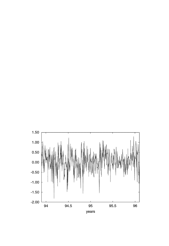
provided in Fig. 1. The mean return is equal to 0.043% and the standard deviation to
0.48%. The greatest positive and negative returns are 1.30% and

1.82%, the last

observation is 1.30% and the last but one observation is

1.07%. The index (not

reproduced here) exhibits a downward trend over the first half of the sample period and an
upward trend after.

Fig. 1. Brussels spot market index return (23/11/93 to 30/01/96).

L. Bauwens, M. Lubrano / Journal of Empirical Finance 9 (2002) 321–342

329

3.1. Models and likelihood function

The general form of the three models that we estimate and their likelihood functions are

given by:

¼ qy

ﬃﬃﬃﬃ

ð0; 1Þ

¼ gð y

;

ðh; yÞ~

¼2

1=2
t

exp

¼2

ð17Þ

For the symmetric model, h

is given in Eq. (10). We use a uniform prior on finite intervals

for all the parameters. The posterior moments exist provided h

is strictly positive and

finite. This implies that the range of integration for x starts at a strictly positive value.

The two variants of the symmetric GARCH model (10) we shall consider adopt the

common formulation

¼ x þ a

ð1 f

Þ þ a

þ bh

ð18Þ

The model of Glosten et al. (1993) assumes an asymmetry between positive and negative
shocks and is obtained by defining f

as a Heavyside function with

if u

< 0

otherwise:

ð19Þ

The leverage effect is present in Eq. (18) if a

is larger than a

, so that the news impact

curve is steeper for negative shocks than for positive ones. In this asymmetric model
(hereafter GJR), the impact of shocks on the variance depends on the sign of the shock.
This model was already used in a Bayesian framework by Bauwens and Lubrano (1998)
on weekly data for the Brussels stock index. We use the same type of prior as above.
Posterior moments exist under the same condition provided there are enough observations
in each regime.

The second variant considers the possibility of saturation in an asymmetric model.

Volatility is increased by bigger shocks, but till a certain extent beyond which it stays
constant. This effect is obtained by a smooth transition model introduced in Lubrano
(2001) who replaces the above f

Heavyside function by a smooth exponential transition

function with a threshold:

ðu; c; cÞ ¼ 1 expðcðu cÞ

Þ:

ð20Þ

In this transition function, the threshold c monitors the degree of asymmetry and c the
saturation. In order to get a scale-free c, the quantity u

c has to be normalised by the

standard deviation of y

. This model (hereafter STR) is known to present identification and

estimability problems at both ends of the support of c. For c = 0, the transition function is

L. Bauwens, M. Lubrano / Journal of Empirical Finance 9 (2002) 321–342

330

zero. Consequently, a

becomes not identified. When c

! l, the transition function

becomes a Heavyside function equal to zero for u = c and equal to one otherwise. The
parameter c will tend to pick up an outlier so that the model tends to be equivalent to a
linear GARCH model with a dummy variable for that point. As this is another well defined
model having a positive probability, the posterior density of c is not integrable because its
right tail does not tend to zero quickly enough (see Lubrano, 2001 for a formal proof). We
introduce a gamma prior to solve both problems:

ðcÞ~c

exp

ðc=c

Þ:

ð21Þ

The prior is zero at c = 0 if m > 1 and has an exponentially decaying tail that insures the
existence of posterior moments.

Generally speaking, the problem of existence of posterior

moments arises every time the likelihood function does not go to zero quickly enough or
presents a nonintegrable singularity. This is the case for some simultaneous equation
models and for cointegration models (see Bauwens et al., 1999). For GARCH models, the
likelihood function based on Gaussian errors does not present this kind of pathology. The
problem could have arisen with the STR model only. However, the prior solves the matter
and as anyway we integrate on a finite interval and the function is finite, the resulting
integrals converge.

3.2. Inference results

Classical and Bayesian inference results for the three models are given in Table 1. The

following general comments apply to these results:

(1) Negative shocks have a stronger impact than positive shocks on the next conditional

variance. In the GJR model, the difference k = a

has a posterior mean equal to 0.090

with a standard deviation equal to 0.066. The posterior probability that k is negative is
small (less than 6%). The posterior probability that a

is negative in the STR model is zero.

(2) For the smooth transition model, we chose m = 3 and c

= 0.5 for the gamma prior,

which implies E(c) = 1.5 and Var(c) = 0.75. The posterior density is dominated by the prior.
The coefficient corresponding to positive shocks, a

was set equal to zero, as the

maximum likelihood algorithm could not depart from this starting value. The news impact
curve (not reported here) is not flat for positive shocks as the transition between the two
regimes is smooth. Note that the news impact curves of the GJR and the smooth transition
model are fairly similar, but with a difference in the right tail that implies a further
dampening influence of large positive shocks for the smooth transition model compared to
the GJR model.

(3) Classical estimates and Bayesian posterior moments are very close for the

regression parameters l and q. Note the differences for x and b because the posterior
densities of these two parameters are rather skewed. The gamma prior on c entails a much
smaller posterior mean and standard deviation than their classical counterparts for c and c.
However, Bayesian posterior standard deviations are substantially larger for the GARCH

Note that with m = 1, we get as a particular case the exponential prior used for instance by Geweke (1993) in

a regression model with Student errors.

L. Bauwens, M. Lubrano / Journal of Empirical Finance 9 (2002) 321–342

331

Table 1
Inference in the GARCH models

Model

Classical results
Basic

0.031 [0.019]

0.24 [0.044]

0.0075 [0.0053]

0.91 [0.036]

0.056 [0.019]

GJR

0.027 [0.020]

0.25 [0.045]

0.0098 [0.0069]

0.90 [0.042]

0.021 [0.021]

0.083 [0.031]

STR

0.028 [0.019]

0.24 [0.045]

0.0081 [0.0058]

0.90 [0.038]

0.0 [ – ]

0.088 [0.031]

2.17 [4.36]

1.16 [0.46]

Bayesian results
Basic

0.032 [0.020]

0.24 [0.046]

0.028 [0.020]

0.80 [0.11]

0.082 [0.037]

GJR

0.026 [0.020]

0.25 [0.047]

0.027 [0.020]

0.80 [0.11]

0.039 [0.033]

0.13 [0.064]

STR

0.028 [0.020]

0.25 [0.047]

0.028 [0.016]

0.79 [0.088]

0.0 [ – ]

0.13 [0.063]

1.15 [0.81]

0.91 [0.44]

‘Basic’ is the model defined by Eq. (17) and h

in Eq. (10), ‘GJR’ corresponds to Eqs. (17) – (19), and ‘STR’ to (Eqs. (17), (18) and (20). Classical results are maximum

likelihood estimates and standard errors (in brackets). Bayesian results are posterior means and standard deviations (in brackets). Five thousand draws (plus 750 for
warming) were used for the Griddy – Gibbs algorithm (see Bauwens and Lubrano, 1998). The average computing time is 10 min on a Pentium 1Gh. All computations were
done with GAUSS.

L.
Bauwens,

Lubrano

Journal

of
Empirical

Finance

(2002)

321–342

332

parameters x, a and b, giving certainly a better account of parameter uncertainty than that
provided by classical standard errors.

3.3. Comparing estimated volatilities

We can compute the implied marginal variance for each empirical model. For the Q-

measure, the formulae are given by Eqs. (11), (25), and (27), depending on the model. For
the P-measure, the usual formulae for GARCH models apply (set q = 0 in the denominators,
and set the numerators to x). These variances can be used in the BS formula if one decides
to ignore heteroskedasticity. They should be compared to the empirical variance (0.231).

Table 2 presents the classical and the Bayesian results for the three models. They are

obtained as transformations of the original parameters. Classical results are evaluated at
the MLE and are thus very unreliable if the estimates are close to the nonstationarity
boundary, which corresponds to a denominator close to 0 in the formula. This produces the
relatively large values for the STR model (as its estimates are close to the nonstationarity
boundary). Bayesian marginal moments are obtained as a transformation of every draw of
the posterior density, the expectation being taken at the end (instead of computing the
marginal moments at the posterior expectation of the parameter). They are truncated
moments since the draws that do not verify the stationarity condition are rejected. The
reported posterior probabilities indicate that a small amount of draws had to be rejected
and that the processes can be taken as stationary. Due to the way they are computed, the
Bayesian results are more reliable than the classical ones, especially for the STR model.

The results indicate a significant increase in the marginal volatility when risk neutralisa-

tion is taken into account. The adoption of the asymmetric model in its GJR version hardly
makes a difference. On the contrary, the smooth transition model yields about 50% higher
marginal variances because this model implies a higher probability of nonstationarity.

4. Predictive option prices: computations and results

Predictive option pricing requires the evaluation of a high-dimensional integral as we

have to take the expectation both over the parameter space of h and over future returns. As
indicated before, Geweke (1989) has proposed a simulation algorithm to compute the
integrals in Eq. (14). In order to adapt this algorithm, we must take into account the fact
that the original GARCH model has an autoregressive mean and that the prediction has to

Table 2
Marginal volatilities for the empirical models

Basic

GJR

STR

Classical r

0.232

0.260

0.220

0.237

0.892

2.110

Bayesian r

0.249

0.299

0.249

0.319

0.375

0.470

Prob. stat.

0.986

0.976

0.984

0.979

0.874

0.837

Moments and posterior probabilities for P and Q are computed on the same set of draws, supposing that r = 0 for
the Q case. Prob. stat. is the posterior probability of stationarity.

L. Bauwens, M. Lubrano / Journal of Empirical Finance 9 (2002) 321–342

333

be done with the risk-neutralised GARCH process. We first detail the predictive skedastic
function for each model and then give the simulation algorithm. The rest of the section is
devoted to empirical results.

4.1. Predictive skedastic functions

Let us write down the risk-neutralised predictive skedastic function for each of the three

proposed empirical models. The general formula is given in Eq. (9) and we have justified
previously the choice l

= l + qy

. For the symmetric GARCH, we get

¼ x þ av

þ bh

;

ð22Þ

where

¼ ð1 qÞr l þ e

ﬃﬃﬃﬃﬃﬃﬃﬃﬃﬃ

;

ð23Þ

and e f N(0,1). For the asymmetric models, we have

¼ x þ a

þ ða

Þv

þ bh

ð24Þ

Let us first consider the case where f

is the Heavyside function ( = 1 if v

is negative

and 0 otherwise). We show in Appendix A that the predictive variance of y

Var

ðy

Þ ¼

þ ½ð1 qÞr l

ða

þ a

Þ=2

ð1 þ q

Þða

þ a

Þ=2 b

;

ð25Þ

provided

ð1 þ q

Þða

þ a

Þ=2 þ b < 1:

ð26Þ

When f

is the exponential smooth transition function defined in Eq. (20), the predictive

variance is

Var

ðy

Þ ¼

þ a

½ð1 qÞr l

ð1 þ q

Þa

;

ð27Þ

provided

ð1 þ q

Þa

þ b < 1:

ð28Þ

These two stationarity conditions, together with a + b < 1 for the symmetric case, serve to
reject draws of h for which stationarity is not verified.

4.2. Computational aspects

The algorithm given in Table 3 produces N M draws of the predictive density of P

. It

uses draws from the posterior density of h that are easily obtained provided a Monte Carlo
method has been used to make inference and that the draws have been stored. The draws

L. Bauwens, M. Lubrano / Journal of Empirical Finance 9 (2002) 321–342

334

that do not satisfy the stationarity conditions stated in the previous subsection have to be
rejected. The inner loop on k approximates the inner integral in y while the outer loop on i
approximates the outer integral in h.

This algorithm can be improved (variance reduction) by implementing the technique of

‘‘antithetic variates’’ (see, e.g. Davidson and MacKinnon, 1993, Chap. 21 and also Hull
and White, 1987). The draws of e are used twice in the inner loop, but with an opposite
sign the second time. Let us call P

and P

the two option prices obtained corresponding

to one draw of h. The price that is finally delivered is P

= ( P

+ P

)/2. Geweke (1989)

shows that when N

! l, the value of M no longer matters to obtain consistent results.

However, as h is typically costly to obtain, there is an incentive to take M greater than 1. In
the example treated below, we took N = 5000 (minus the number of rejections) and M = 50.
As detailed in Section 2.4, we retained only every tenth draw of h to limit the
autocorrelation in h generated by the MCMC algorithm. Consequently, the final number
of draws used for prediction is 5000/10 50 = 25 000. In a classical approach, N would be
equal to 1 as h is fixed at the maximum likelihood estimate and M would be chosen large.
Duan (1996), for instance, uses M = 5000.

The predictive density of the payoff function of the option can be approximated by a

kernel estimate of the N M simulated values of that function. Option prices are computed
as the discounted sample mean of P

as given in Eq. (16) with r = 0.

4.3. Option pricing for the Brussels spot index

We report in Table 4 the predictive option prices for the Brussels spot index for three

different maturities: 15, 30 and 60 days, starting at the end of the observed sample minus
two observations (because this n

2 observation is largely negative and thus constitutes a

good example for the asymmetric models). A 15-day maturity is certainly very short for an
option, but one should remember that its price is also the price of any option 15 days
before its maturity. When we observe a real option market for say 3-month options, the

Table 3
Simulation algorithm for option prices with maturity ns periods ahead of t

i = 1, N

f u(h j y)

k = 1, M

e f N

(0, I

)

= x

+ a

( y

)

+ b

¼ r þ e

ﬃﬃﬃﬃﬃﬃﬃ

= x

+ a

(ys

yt)

+ b

¼ r þ e

ﬃﬃﬃﬃﬃﬃﬃ

j = 3, ns

= x

+ a

(ys

)

+ b

¼ r þ e

ﬃﬃﬃﬃﬃﬃ

j = j + 1
S

¼ S

ns
j

¼1

ð1 þ ys

100

= (1 + r)

max(S

K, 0)

k = k + 1

i = i + 1

L. Bauwens, M. Lubrano / Journal of Empirical Finance 9 (2002) 321–342

335

market is very quiet at the beginning of the option life, but gets very active a few weeks
before the maturity. We have supposed that the riskless interest rate r was equal to zero.
We took the normalisation rule S

= 1 and considered a range of moneyness (S

/K) between

0.959 and 1.045.

We have computed the Monte Carlo standard errors. We do not give them in full detail,

but the following indications are useful. For out-of-the-money options, t statistics are
slightly above the maturity (20 for a 15-day maturity, etc). For at-the-money options, they
are all of the order of 200. For in-the-money options, they are between 1000 and 15000.
Translated in term of precision for the estimates, a 1% precision needs a t of 200, and 10%
precision a t of 20 (if the mean is 0.010, then 0.011 is at the border of the 95% confidence
interval in the case of a 10% precision). Every time we shall say that two option prices are
different, we mean that the second is not contained within a 95% confidence interval of the
first.

We computed but do not report classical results. Broadly speaking, classical estimates

of the option prices are close the Bayesian predictive means. They are slightly different
for out-of-the-money options. The differences are weaker for at-the-money options. We
can say that there are no noticeable differences for in-the-money options, except when
using the STR model. This is a sign of the robustness of the risk-neutral pricing
methodology.

Table 4
Predictive call option prices for Brussels stock index

Maturity (days)

Moneyness

0.959 (out)

1.000 (at)

1.045 (in)

Basic
15

0.00021 (0.02)

0.00013

0.0081 (0.50)

0.0076

0.0430 (0.98)

0.0430

0.00099 (0.07)

0.00079

0.0113 (0.50)

0.0108

0.0437 (0.94)

0.0435

0.00315 (0.14)

0.00278

0.0159 (0.49)

0.0153

0.0457 (0.86)

0.0453

GJR
15

0.00018 (0.02)

0.00015

0.0084 (0.51)

0.0077

0.0431 (0.91)

0.0430

0.00088 (0.07)

0.00081

0.0116 (0.51)

0.0109

0.0440 (0.93)

0.0435

0.00306 (0.14)

0.00283

0.0162 (0.50)

0.0153

0.0461 (0.86)

0.0453

STR
15

0.00020 (0.02)

0.00038

0.0082 (0.50)

0.0090

0.0430 (0.98)

0.0432

0.00089 (0.06)

0.00158

0.0113 (0.50)

0.0128

0.0438 (0.94)

0.0442

0.00283 (0.14)

0.00455

0.0159 (0.50)

0.0180

0.0457 (0.86)

0.0469

is the predictive option price defined in Eq. (16). Numbers in parentheses are the probabilities of exercise of

the option. BS

is the mean of Eq. (5) evaluated at the marginal variance under measure P, the mean being taken

with respect to h. Moneyness is S

/K. It is equal to 1 for options at the money, smaller than 1 for out-of-the-

money options, and larger than 1 for in-the-money options (at time t). The computing time (with GAUSS on a
Pentium 350Mh) using 500 (N) times 50 (M) repetitions is 77 s with the basic model for a maturity of 60 days,
shorter maturities being obtained as a by-product. This time goes up to 102 s for the GJR model and 109 s for the
STR model.

L. Bauwens, M. Lubrano / Journal of Empirical Finance 9 (2002) 321–342

336

Let us now compare the prices obtained using the predictive method and those obtained

with the expectation of the BS formula

, both reported in Table 4. For in-the-money

options, there are no economically significant differences. For at-the-money options,
significant differences are appearing (more than a 5% difference in price when the
numerical precision is of the order of 1%), but these differences are decreasing with
maturity. The BS formula underprices options for the basic and GJR models, but
overprices it for the STR model. For out-of-the-money options, the BS formula under-
prices strongly short maturities (38% for 15 days) for the basic model. This underpricing
attenuates with maturity and when the GJR model is used. This means that the GJR model
gives a better account of the marginal volatility of the underlying security. With the STR
model, the BS formula strongly overprices, showing that the marginal volatility is not
estimated with a satisfactory accuracy in this model. All these results amplify when we
plug in the BS formula the classical estimate of the marginal volatility.

We report in Table 5 the implied mean predictive volatilities. This is defined as the

mean, over the number of periods to maturity, of the predictive volatilities hs

¼1

ð29Þ

The predictive volatility in period j (between t and t + ns) is the mean of the volatilities hs

generated according to the simulation algorithm described in Table 3:

¼1

ð30Þ

For the three models, the mean predictive volatilities decrease with maturity. The decrease
is due to the configuration of the sample and convergence results from stationarity. These
mean conditional volatilities converge also to smaller values than the computed marginal
volatilities reported in Table 2. The latter were computed as truncated moments (as
explained in Section 3.3). Table 5 reveals no serious differences (not more than 5%)
between the models, but Table 2 reveals a similar picture for the Bayesian estimates of the
basic and the GJR models. Therefore, the differences we have found between the BS and
the predictive pricing methods for out-of-the-money options come just from the fact that
the BS formula is too sensitive to variations of the volatility.

We computed E

(BS[r(h)]). This is the posterior expectation of the BS formula of Section 2.1. It is

different from the Hull and White (1987) approach of Section 2.2.

Table 5
Mean predictive volatilities

15 days

30 days

60 days

Basic

0.282

0.275

0.270

GJR

0.304

0.290

0.282

STR

0.291

0.278

0.269

The mean predictive volatility is defined in Eqs. (29) and (30) together with Table 3.

L. Bauwens, M. Lubrano / Journal of Empirical Finance 9 (2002) 321–342

337

Looking at the results given in Table 4, we note that the expected option prices are not

much different between the basic and the two asymmetric models (within the Monte Carlo
precision). On one side, this gives confidence about the robustness of the predictive
pricing method compared to a misuse of the BS formula as reported above. On the other
side, this is disrupting as one may think that asymmetric models would have produced a
different pricing in the presence of negative shocks and short maturities. However, we
must not forget that the Bayesian approach gives not only an expected option price, but
also a complete density. Considering the complete density may shed some more light on
the question.

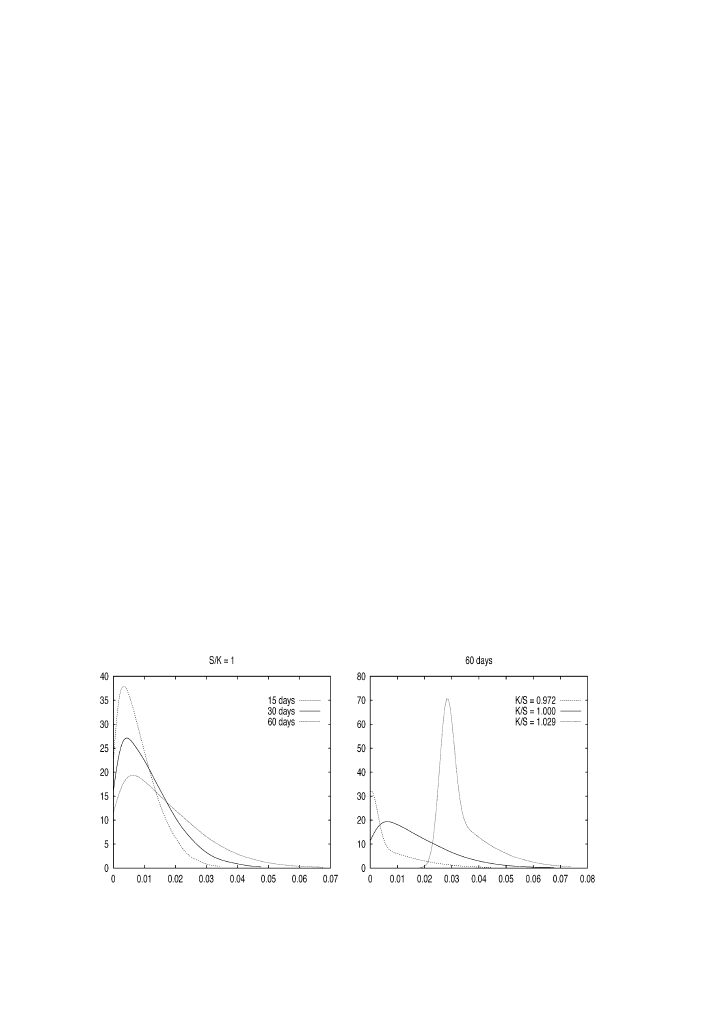
The interest of our approach is to provide a probability distribution with respect to

which (observed) option prices can be assessed, namely the predictive distribution of the
option payoff function (the expected value of this distribution being the predictive option
price). We provide in Fig. 2 (left panel) the computed predictive densities for the three
maturities and a strike of 1. Actually, this type of density has a discrete component and a
continuous one: the discrete component is at zero and corresponds to the fact that the
payoff function is the maximum of zero and the difference S

K, and the continuous part

corresponds to the positive values of this difference. Only the continuous part is drawn on
the figures so that the densities integrate to the probability of being positive (e.g. about
equal to 0.5 for at-the-money options). The probability at zero is the predictive probability
that the option will not be exercised. It is evaluated by the proportion of null values of the
payoff function in the total number of simulations (N M). The complementary proba-
bilities are reported in Table 4 (see the numbers in parentheses). The message that is
apparent from the left panel of Fig. 2 is that, at least for the observed sample, uncertainty
increases with maturity while the predictive mode does not increase significantly. On the
contrary, as shown in the right panel of Fig. 2, the option price is very sensitive to the
moneyness (given there for a maturity of 60 days and a smaller range of moneyness than
that displayed in Table 4).

It is difficult to detect an influence of modelling asymmetry on option prices. For out-

of-the-money options and at-the-money options, there is no significant differences in the

Fig. 2. Predictive density for the payoff function for the basic model.

L. Bauwens, M. Lubrano / Journal of Empirical Finance 9 (2002) 321–342

338

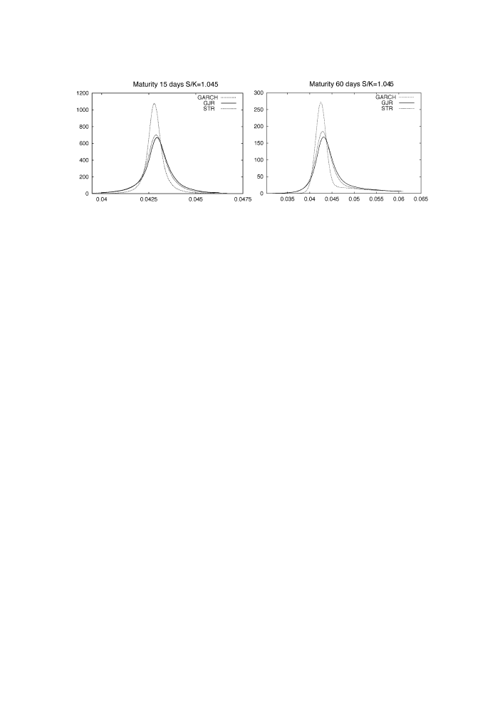
graphs of the predictive payoffs. However, surprisingly for options largely out-of-the-
money as those reported here, a difference appears as shown in Fig. 3. The two
asymmetric models perform similarly (which is not so surprising) but ignoring asymmetry
apparently gives a too-high precision about the mean option price for our particular
sample. This effect seems to be valid independently of the maturity.

5. Conclusion

This paper shows how option prices can be evaluated from a Bayesian viewpoint

using an econometric model to predict the future stock price and volatility. The option
price provided by our method is the predictive expectation of the payoff function of the
option. Other characteristics of options (delta, gamma,. . .) could be predicted. Our
method delivers the predictive distribution of the payoff function for a given econo-
metric model. This probability distribution could be useful to market participants who
wish to compare the model prediction to potential prices on the market or to other
predictions.

This paper also shows that in a Bayesian approach, an additional source of uncertainty

is taken into account, which has consequences on the measure of volatility and as a result
on option pricing. It shows how the predictive method finally produces a better evaluation
of the actual volatility contained in the data when there is a large uncertainty on marginal
measures due to nearly nonstationarity. Because of this nearly nonstationarity, using a
marginal measure to be plugged in the BS formula can be very dangerous.

Finally, this paper shows that modelling asymmetry does not seem essential for pricing

options nearly at the money, but may have a significant impact on the dispersion of the
predicted prices for in-the-money options.

Acknowledgements

Support of the European Commission Human Capital and Mobility Program through

the network ‘‘Econometric inference using simulation methods’’ is gratefully acknowl-

Fig. 3. Impact of the model choice on the predictive density for the payoff function.

L. Bauwens, M. Lubrano / Journal of Empirical Finance 9 (2002) 321–342

339

edged. While remaining responsible for any error, the authors wish to thank Christian
Hafner, Robert Kast, Valentin Patilea, Peter Schotman, and seminar participants at
Erasmus University Rotterdam, Humboldt-University Berlin, and CORE for useful
remarks and suggestions.

This paper presents research results of the Belgian Program on Interuniversity Poles of

Attraction initiated by the Belgian State, Prime Minister’s Office, Science Policy
Programming. The scientific responsibility is assumed by the authors.

Appendix A. Variance and stationarity condition for risk-neutralised GARCH
processes

The marginal variance of y in GARCH processes is computed using the law of iterated

expectations and the fact that the process is supposed to be stationary. See Bauwens et al.
(1999, Chap. 7) for details.

Let us write down the risk-neutralised predictive process for each of the three proposed

empirical models. We have first

¼ r þ e

ﬃﬃﬃﬃﬃ

fN ð0; 1Þ:

ð31Þ

For the skedastic function, the general formula is given in Eq. (9) and we have justified
previously the choice l

= l + qy

. For the symmetric GARCH, the predictive skedastic

function is

¼ x þ av

þ bh

;

ð32Þ

where

¼ ð1 qÞr l þ e

ﬃﬃﬃﬃﬃﬃﬃﬃﬃﬃ

ð33Þ

The predictive expectation of h

is given by

ðh

Þ ¼ x þ aEðv

Þ þ bEðh

Þ:

ð34Þ

We have essentially to compute

ðv

Þ ¼ ½ð1 qÞr l

þ E

ﬃﬃﬃﬃﬃﬃﬃﬃﬃﬃ

¼ ½ð1 qÞr l

þ E½e

þ q

¼ ½ð1 qÞr l

þ ð1 þ q

ÞE½h:

ð35Þ

Solving for E(h), we get Eq. (11)

For the GJR asymmetric model, the skedastic function is

¼ x þ a

þ ða

Þv

þ bh

;

ð36Þ

L. Bauwens, M. Lubrano / Journal of Empirical Finance 9 (2002) 321–342

340

where f

is the Heavyside function that is one if v

< 0 and zero otherwise. We have to

compute

ðh

Þ ¼ x þ a

ðv

Þ þ ða

ÞEðv

j v

Þ þ bEðh

Þ:

ð37Þ

We have already got E(v

) from the symmetric case. It thus remains to compute the

truncated conditional expectation E(v

< 0)

ðv

j v

Þ ¼ ðð1 qÞr lÞ

þ E

ﬃﬃﬃﬃﬃﬃﬃﬃﬃﬃ

Supposing that the distribution of v

is symmetric and that the function e

ﬃﬃﬃﬃﬃﬃﬃﬃﬃﬃ

is also symmetric, we have

ﬃﬃﬃﬃﬃﬃﬃﬃﬃﬃ

¼ ð1 þ q

ÞEðhÞ=2;

which is just half the quantity obtained in the symmetric case. Regrouping partial results,
we get Eqs. (25) and (26).

When f

is a smooth transition function, it seems natural to study the stationarity

condition for the limiting case when c

! l. With an even smooth transition function, the

limiting case is the GJR model. When the smooth transition function is the asymmetric
exponential function defined in Eq. (20), it must be noted that the model becomes linear
when c

! l. Consequently, E(h) and the stationarity condition in this case are identical to

the results derived for the standard GARCH(1,1) model, just replacing a by a

(see Eqs.

(27) and (28)).

References

Bauwens, L., Lubrano, M., 1998. Bayesian inference on GARCH models using the Gibbs sampler. The Econo-

metrics Journal 1, C23 – C46.

Bauwens, L., Lubrano, M., Richard, J.-F., 1999. Bayesian Inference in Dynamic Econometric Models. Oxford

Univ. Press, Oxford.

Campbell, J., Lo, A.W., MacKinley, A.C., 1997. The Econometrics of Financial Markets. Princeton University

Press, Princeton.

Cox, J.C., Ross, S.A., 1976. The valuation of options for alternative stochastic processes. Journal of Financial

Economics 3, 145 – 166.

Davidson, R., MacKinnon, J.G., 1993. Estimation and Inference in Econometrics. Oxford Univ. Press, Oxford.
Duan, J.C., 1995. The GARCH option pricing model. Mathematical Finance 5, 13 – 32.
Duan, J.C., 1996. Craking the smile. Risk 9, 55 – 59.
Duan, J.C., 1999. Conditionally fat-tailed distributions and the volatility smile in options. Working Paper, Depart-

ment of Finance, Hong-Kong University.

Engle, R.F., Lilen, D.M., Robin, R.P., 1987. Estimating time varying risk premia in the term structure: the ARCH-

M model. Econometrica 55, 391 – 407.

L. Bauwens, M. Lubrano / Journal of Empirical Finance 9 (2002) 321–342

341

Garcia, R., Renault, E., 1997. A note on hedging in ARCH and stochastic volatility option pricing models.

Working Paper 97s-13, CIRANO, Universite´ de Montre´al.

Geweke, J., 1989. Exact predictive densities for linear models with ARCH disturbances. Journal of Econometrics

40, 63 – 86.

Geweke, J., 1993. Bayesian treatment of the independent Student-t linear model. Journal of Applied Econometrics

8, 19 – 40 (Supplement).

Glosten, L.R., Jagannathan, R., Runkle, D.E., 1993. On the relation between the expected value and the volatility

of the nominal excess return on stocks. Journal of Finance 48, 1779 – 1801.

Hafner, C.M., Herwartz, H., 2001. Option pricing under linear autoregressive dynamics, heteroskedasticity and

conditional leptokurtosis. Journal of Empirical Finance 8, 1 – 34.

Heston, S.L., Nandi, S., 2000. A closed-form GARCH option valuation model. The Review of Financial Studies

13, 585 – 625.

Hull, J., White, A., 1987. The pricing of options with stochastic volatilities. Journal of Finance 42, 281 – 300.
Kallsen, J., Taqqu, M.S., 1998. Option pricing in ARCH-type models. Mathematical Finance 8, 13 – 26.
Lubrano, M., 2001. Smooth transition GARCH models: a Bayesian perspective. Recherches Economiques de

Louvain 67, 257 – 287.

Mahieu, R.J., Schotman, P.C., 1998. An empirical application of stochastic volatility models. Journal of Applied

Econometrics 13, 333 – 360.

Noh, J., Engle, R.F., Kane, A., 1994. Forecasting volatility and option prices of the S & P 500 index. Journal of

Derivatives, 17 – 30.

Pagan, A., 1996. The econometrics of financial markets. Journal of Empirical Finance 3, 15 – 102.
Terasvirta, T., 1996. Two stylised facts and the GARCH(1,1) model. Working Paper 96, Working Paper Series in

Economics and Finance, Stockholm School of Economics.

L. Bauwens, M. Lubrano / Journal of Empirical Finance 9 (2002) 321–342

342

Document Outline

Introduction
Predictive option pricing: principles
GARCH models for Brussels stock index
Predictive option prices: computations and results
Conclusion
Acknowledgements
Variance and stationarity condition for risk-neutralised GARCH processes
References

Wyszukiwarka

Podobne podstrony:
bayes v1 prezentacja
duration analysis v1 artykul id Nieznany
bayes v1 prezentacja
nieparametryczne v1 artykul
markov v1 artykul
gmm v1 artykul a
panele v1 artykul
gmm v1 artykul b
PO wyk07 v1
s10 v1
s7 4 v1
s9 3a v1
dodatkowy artykul 2
ARTYKUL
Prezentacja v1

więcej podobnych podstron

bayes v1 artykul

Document Outline