panele v1 artykul

The Predictive Value of Subjective Labour Supply Data:

A Dynamic Panel Data Model with Measurement Error

Rob Euwals

IZA, Bonn, and CEPR, London.

November 2001

Abstract

This paper tests the predictive value of subjective labour supply data for adjustments in working

hours over time. The idea is that if subjective labour supply data help to predict next year’s working

hours, such data must contain at least some information on individual labour supply preferences.

This informational content can be crucial to identify models of labour supply. Furthermore, it can be

crucial to investigate the need for, or, alternatively, the support for laws and collective agreements

on working hours flexibility. In this paper I apply dynamic panel data models that allow for

measurement error. I find evidence for the predictive power of subjective labour supply data

concerning desired working hours in the German Socio-Economic Panel 1988-1996.

KEYWORDS: Labour Supply, Subjective Data, Measurement Error, Dynamic Panel Data Models

JEL CLASSIFICATION: C23, J22

CONTACT:

euwals@iza.org

I wish to thank John Haisken-DeNew, Astrid Kunze, Markus Pannenberg, Rainer Winkelmann and my colleagues at IZA for their helpful advice and

valuable comments. The author gratefully acknowledges DIW for providing the data.

1. Introduction

This paper aims at testing the predictive value of subjective labour supply data for adjustments in

working hours over time. The idea is that if subjective labour supply data help to predict next year’s

working hours, such data must contain at least some information on individual labour supply

preferences. This informational content can be crucial to identify models of labour supply.

Furthermore it can be crucial to investigate the need for, or, alternatively, the support for laws and

collective agreements on working hours flexibility. To test the predictive value, I apply panel data

models that account for measurement error.

In the mainstream economic literature empirical strategies are typically based on the idea that

statistical inference should be based on ‘revealed preferences’, i.e. on ‘realised behaviour’. This

methodology is built on the general belief of (most) economists that it is only then that individuals

have to reveal their true preferences. However, in several fields of economics it has become clear

that only the informational content of realised behaviour can be limited to identify individual

preferences. The use of subjective data is then an alternative methodology for applications with

identification problems.

Subjective labour supply data can, for instance, be helpful to identify

individual labour supply preferences. In an early example of this methodology, Ham (1982) uses

subjective data on constraints on working hours in the Michigan Panel Study of Income Dynamics

to identify a labour supply model with underemployment. His approach is followed and extended by

many authors, including Ilmakunnas and Pudney (1990), Kahn and Lang (1991), Stewart and

Swaffield (1997), and Euwals and Van Soest (1999). Another example for the use of subjective

labour supply data (which is, however, less frequently published in the international literature) is the

investigation of the need for and/or the support for laws and collective agreements on working

hours flexibility. Examples, using the same data source as this study, are, for instance, Hunt (1998),

Bell and Freeman (2000), and Pannenberg and Wagner (2001).

Whatever the reason is for subjective data being used – one should always investigate how credible

the data really are. A way of testing their informational content is to test their predictive value.

this paper I examine whether subjective data on desired working hours have predictive power for

next year’s working hours, conditional on this year’s working hours. Since the data source for this

For more extensive arguments favouring this idea, see, for instance, Manski (2000) and Kapteyn and Kooreman (1992).

See Juster (1966) for an early and influential study using this idea. He finds no predictive power for subjective data on buying intentions in the US

Survey on Consumer Finances.

study – the German Socio-Economic Panel (GSOEP) – provides subjective labour supply data over

a long time period I will use panel data techniques. An advantage of these techniques is that they

allow for the incorporation of measurement error in observed variables.

The remainder of the paper is organised as follows: Section 2 discusses the labour supply data that

are available in the GSOEP. Section 3 introduces the analytical framework for testing the predictive

value of subjective labour supply data. Next, Section 4 presents descriptive statistics of the data,

while Section 5 presents estimation results. Section 6 concludes.

[Insert Table 1 about here]

2. Survey Questions

The data source of this study is the German Socio-Economic Panel (GSOEP), which is a nationally

representative annual panel on the household level. The first wave was conducted in 1984, and it is

currently still running. Data on individual working time are collected on a yearly basis using the

same questions in every year since 1988, which obviously facilitates a panel data analysis. The

question concerning the subjective labour supply data was not conducted in the first year of the

panel, 1984, nor was it conducted in 1996. Since the data of the year 1996 are useful for observing

adjustments in actual working hours over time, this study uses the data from 1988 to 1996.

For the interpretation of the results a good understanding of the data on working time is crucial.

This section presents the survey questions on actual and desired working time. Questions (1) to (3)

of Table 1 concern the questions on actual working hours. The answers to these three questions by

individual i at time t are denoted by contractual working hours hc

, total working hours ht

, and the

overtime rule or

. Due to the increasing popularity of working time accounts, compensation of over-

time in a certain period with extra time off in another period is quite common in Germany. In the

data used for this study the percentage of men and women that are compensated by extra time off

(answer ‘B’) increased from 22% and 30%, respectively, in 1988 to 34% and 45% in 1996.

Furthermore the percentage of men and women that are partly paid and partly compensated by extra

time off (answer ‘C’) increased from 11% and 7%, respectively, in 1988 to 17% and 10% in 1996.

This is an improvement over Euwals et al. (1998), where the time-period covered by the data was too short for such an approach.

The answer to question (4) of Table 1 by individual i at time t is denoted by desired working hours

. Comparing this question to questions (1) to (3) shows that a comparison of desired working

hours hd

to the outcomes on actual working hours is not straightforward: It is not clear for which

outcome the desired working hours hd

should have predictive value. One interpretation of question

(4) is that due to the explicit reference to a budget constraint (“…considering analogous changes of

your labour income…”), desired working hours hd

refer to the paid part of working hours only. On

the other hand, respondents might take into account that certain pecuniary rewards (like bonus

payments and promotions) partly depend on unpaid overtime, which means desired working hours

relate to total – paid and unpaid – actual working hours. The references of Section 1 that use the

same data source all stick to the latter interpretation. But to facilitate this concern I will define two

kinds of outcome variables on actual working hours: total actual hours ht

, which are observed, and

paid actual hours hp

. The measurement of paid actual hours is somewhat problematic as choice ‘C’

of question (3) does not state how much of the overtime is paid. I use the following approximation:

(1) hp

= hc

+ I( or

=‘A’) (ht

- hc

) + ½ I( or

=‘C’) (ht

- hc

)

with I( or

=‘A’) an indicator function for individual i at time t giving answer ‘A’ to the question on

the overtime rule. In case of answer ‘C’ I assume that half of the overtime is paid.

3. Panel Data Models with Measurement Error

In this section we formulate an empirical model that is able to test the predictive value of subjective

labour supply data, and that explicitly allows for measurement error in observed variables. We

develop an estimation procedure for the model by using the literature on dynamic panel data models

where measurement error can be incorporated by exploiting the time-dimension of the panel data.

The underlying idea, and crucial assumption, is that measurement error is uncorrelated over time so

that variables of time periods other than the time period of interest can be used as instruments. See

Griliches and Hausman (1986) for an early example exploiting this idea, and see Wansbeek (2001)

for a recent example.

The next subsection formulates an empirical model that explains actual working hours from lagged

actual and lagged desired working hours. For reasons discussed later, the second subsection

formulates an empirical model that explains the adjustment in actual working hours over time from

the lagged deviation between desired and actual working hours.

3.1 A Dynamic Panel Data Model with Measurement Error

We specify an empirical model to explain actual working hours by lagged actual and lagged desired

working hours. Define ha

as the true actual working hours (i.e. true total working hours ht

true paid working hours hp

) of individual i at time t, and hd

as the true desired working hours of

individual i at time t. Define the following model:

(2) ha

= β

+ β

it-1

+ β

it-1

+ ε

with ε

an idiosyncratic error term, which we assume to be uncorrelated over time, and ε

individual specific error term.

Note that the error terms relate to true actual working hours, and

have nothing to do with measurement error. For example, the individual specific error term might

partly represent individual specific effects in labour supply preferences where certain individuals

might prefer to work more hours than other individuals. For our test on the predictive value of the

subjective labour supply data concerning desired working hours, the parameter of interest is β

. The

null hypothesis of the test is β

=0, which means that there is no predictive value. The alternative

hypothesis is β

>0, which means there is predictive value in a way that is economically

interpretable as individuals adjust their actual working hours into the preferred direction.

Note that the empirical model does not include individual labour supply characteristics, like family

characteristics, observed at time t-1. The reason is that we expect these characteristics to have an

impact on true actual working hours ha

through lagged true desired working hours hd

it-1

only.

Therefore incorporation of these characteristics would need a structural simultaneous equations

model in which these characteristics explain the true desired working hours hd

it-1

. As it is not a goal

to explain individual labour supply preferences, this is beyond the scope of this study.

The idea behind the formulation of the model in terms of true actual and desired working hours is

that observed actual and desired hours might be contaminated with measurement error. I define the

relation between true actual and desired working hours (ha

, hd

) and observed actual and desired

working hours (ha

, hd

) as follows:

(3) ha

= ha

+ ν

(4) hd

= hd

+ ν

We will allow the constant term to be time-specific, which is easy to incorporate. See, for instance, Arrelano and Bond (1991).

See Euwals (2001) for a structural simultanous equations model that incorporates adjustments in actual working hours over time and labour supply,

and that is estimated on the basis of the Dutch Socio-Economic Panel.

with (ν

, ν

) idiosyncratic error terms, which we assume to be uncorrelated over time, and (ν

, ν

)

individual specific error terms. The interpretation of these error terms is purely measurement error,

whereby the individual specific error terms allow for systematic (time-constant) over- or under-

reporting of individual i. Substitution of equations (3) and (4) in equation (2) yields:

(5) ha

= β

+ β

it-1

+ β

it-1

+ (ε

+ (1-β

) ν

- β

) + (ε

+ ν

) - (β

it-1

+ β

it-1

)

The resulting model is a dynamic panel data model with some non-standard properties due to the

error structure. Like in the standard dynamic panel data model the lagged dependent variable ha

it-1

is endogenous. The solution offered by the literature is an instrumental variables approach within a

Generalized Method of Moments (GMM) estimation procedure. A particular advantage of this

method is that distributional assumptions are not needed.

As the observed actual and desired working hours of all time periods depend on individual specific

error terms, the first task is to get rid of these individual specific error terms. The common solution

is to take the first difference over time:

(6) ha

- ha

it-1

= β

(ha

it-1

- ha

it-2

) + β

(hd

it-1

- hd

it-2

)

+ (ε

- ε

it-1

) + (ν

- ν

it-1

) - β

(ν

it-1

- ν

it-2

) – β

(ν

it-1

- ν

it-2

)

As we assume all error terms to be uncorrelated over time, serial correlation in the residuals of this

model will only be due to lagged error terms. Now the literature proposes the two-times lagged

dependent variable ha

it-2

as an instrument for (ha

it-1

- ha

it-2

). And indeed is this variable uncorrelated

with the error-term (ε

- ε

it-1

). But the measurement error causes an additional endogeneity problem:

it-2

is correlated with ν

it-2

. Valid instruments are only obtained by using dependent variables that

are at least three-times lagged, for instance ha

it-3

. Notice that the observed desired working hours

are endogenous as well, and that the three-times lagged variable hd

it-3

is a valid instrument.

The goal is to get a consistent estimator for β=[β

, β

]’. Deriving an estimator that is efficient as

possible by using all valid moment restrictions is beyond the scope of the paper.

Instead, we will

follow the convenient and intuitively clear approach of Arellano and Bond (1991), which uses all

valid lagged variables as instruments. First, define ∆ha=ha-ha

-1

as a vector of first differences over

time of the actual working hours stacked for individuals i=1,…,N and time t=1,…,T. The size of the

vector is N(T-3) because for each individual the first three outcomes of the actual working hours

cannot be used. Then define a matrix of instruments Z, which contains sufficiently lagged variables

for (ha

it-1

, hd

it-1

) again stacked for individuals i=1,…,N and time t=1,…,T. The size of this matrix is

N(T-3) x (T-3)(T-2). The GMM estimator takes the following form:

(7)

GMM

= ([∆ha

-1

,∆hd

-1

]’Z W

Z’[∆ha

-1

,∆hd

-1

])

-1

([∆ha

-1

,∆hd

-1

]’Z W

Z’∆ha)

with W

some weighting matrix. For details on the estimation procedure, and in particular on the

relation to Arellano and Bond (1991), see Appendix A.

3.2 A Restricted Panel Data Model with Measurement Error

A disadvantage of the model of Subsection 3.1 is that it is very unrestrictive in the sense that even

the predictive value of lagged actual working hours ha

it-1

might be low. Especially in the case that

the individual specific effects ε

absorb a large part of the variation in actual working hours ha

this might very well happen.

Another interesting test on the predictive value of subjective labour supply data concerning desired

working hours is based on the idea that the lagged deviation between desired and actual working

hours (hd

it-1

- ha

it-1

) might have predictive value for the adjustment of actual working hours over

time (ha

- ha

it-1

). So where the model of Subsection 3.1 considers the predictive value of desired

working hours for the level of actual working hours, the model of this subsection considers the

predictive value for adjustments in actual working hours over time. We define the model as follows:

(8) ha

- ha

it-1

= β

+ β

(hd

it-1

- ha

it-1

) + ε

Note that the model does not include an individual specific effect at this level, as that would imply a

constant rise or fall in the actual working hours of individual i. A way to achieve the model from the

model of Subsection 3.1 is by imposing the restriction β

+β

=1, and by eliminating the individual

specific effect ε

. An interpretation of the restriction on the parameters is that it forces the model to

‘distribute’ the predictive value between the lagged actual and lagged desired working hours, as the

actual working hours are weighted average of these two variables. The time-specific constant term

allows for general upward and downward trends in actual working hours.

Now incorporation of measurement error (see equations (3) and (4)) leads to:

(9) ha

- ha

it-1

= β

+ β

(hd

it-1

- ha

it-1

) - β

(ν

- ν

) + ε

+ (ν

- ν

it-1

) - β

(ν

it-1

- ν

it-1

)

See Baltagi (1995) for an overview of the literature on dynamic panel data models.

The model is not dynamic in the sense that it contains a lagged dependent variable. But due to the

individual specific error terms that relate to measurement error, the model has an endogeneity

problem that is similar to the one of the dynamic panel data model. Take first-differences over time,

and define ∆ha

=ha

-ha

it-1

(10) ∆ha

- ∆ha

it-1

= β

( (hd

it-1

- ha

it-1

) - (hd

it-2

- ha

it-2

) ) + (ε

- ε

it-1

)

+ ( (ν

- ν

it-1

) - (ν

it-1

- ν

it-2

) ) - β

( (ν

it-1

- ν

it-1

) - (ν

it-2

- ν

it-2

) )

As we assume the error terms to be uncorrelated over time, serial correlation in the residuals of this

model will be due to lagged error terms. In the case of no measurement error, two-times lagged

variables (ha

it-2

, hd

it-2

) are valid instruments. An estimation procedure using all variables that are at

least two-times lagged is similar to the one proposed by Arellano and Bond (1991). But the

presence of measurement error makes two-times lagged variables invalid instruments. Instruments

therefore have to be at least three-times lagged. The estimation procedure for this model is similar

to the one described in Subsection 3.1, and we will not go into details here.

[Insert Table 2 and Figures 1.A and 1.B about here]

4. Data

From the GSOEP I select all employed individuals between ages 18 and 60 old that belong to a

West-German household where the household head does not belong to a foreigner group

for all

waves from 1988 to 1996. The selected sample includes employed individuals with valid data for at

least 4 subsequent years.

Individuals that have invalid data on desired working hours in the fourth

or a later year are maintained in the sample because they give an observed outcome on the actual

working hours for that year.

Table 2 shows the sample statistics. For men there is a clear downward trend in paid working hours,

which is consistent with the spreading of working time reductions and time accounts over the

different sectors of the economy in these years. However, total working hours seem to be unaffected

by this decline. For women, the developments are straightforward: There is a downward trend in

Households with a household head belonging to a foreigner group are oversampled in the GSOEP, and we exclude them to avoid weighting.

We ignore selection into and out-of employment, as incorporation would need a model with stronger assumptions.

total, paid and desired working hours. This is due in part to working time reductions and in part to

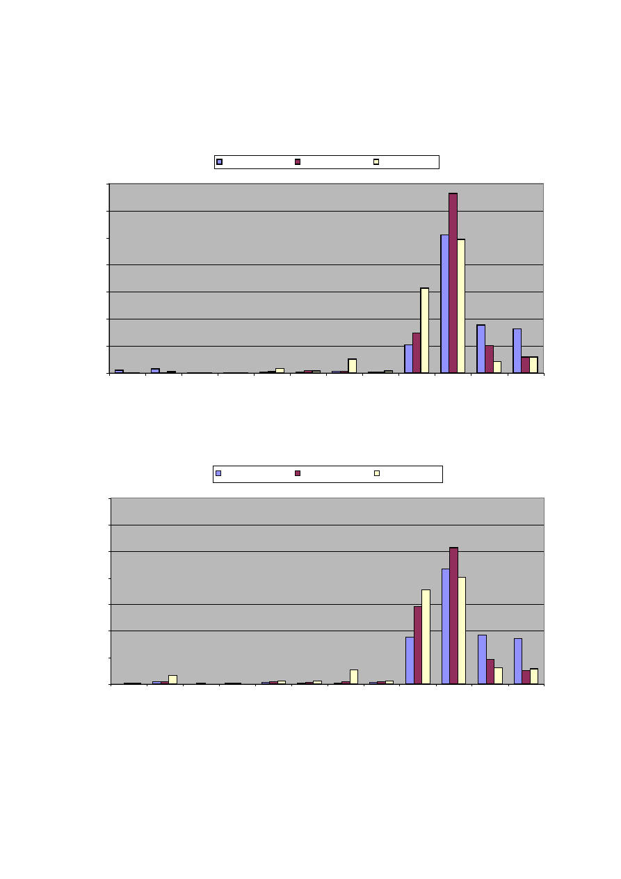
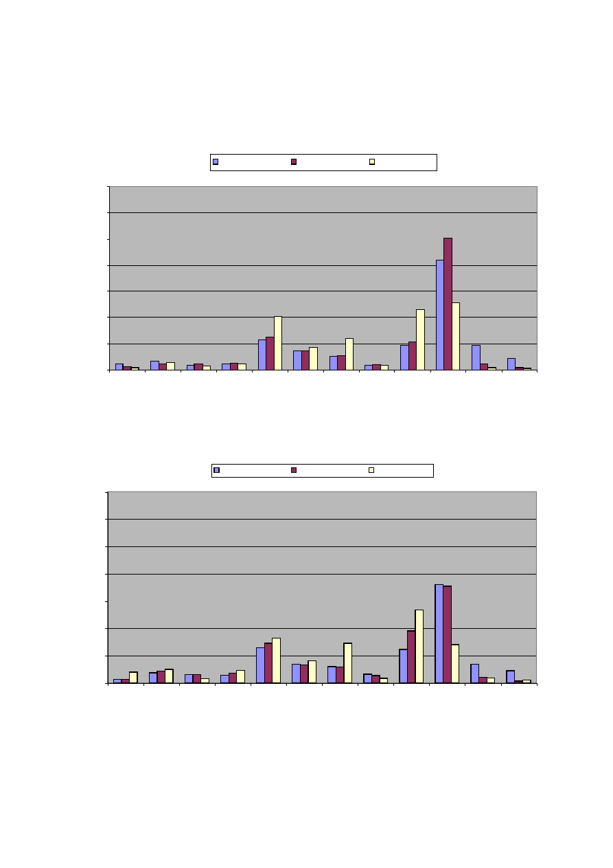
the increasing incidence of part-time employment. Figures 1.A and 1.B show the distribution of

actual and desired working hours. Clearly observable from these figures is the importance of

working time reductions: the number of men working about 36 hours per week increased

substantially between 1988 and 1995. Remarkably, the number of men that want long working

hours (more than 40 hours per week) increased slightly between 1988 and 1995. For women the

figures are much more diversified as a substantial fraction of women works part-time. Still, Figure

1.B expresses some lack of part-time jobs; especially the ‘demand’ for jobs of about 28 hours is

substantially larger than the availability.

Table 3 gives a descriptive answer on whether for all years pooled the subjective data on desired

working hours have predictive value for the next year’s actual working hours. Individuals who have

a wish to work fewer (more) hours have a relatively large probability to work fewer (more) hours

the next year. However, it is hard to tell whether the total or the paid hours are better predicted by

the desired hours. One measure for the success of prediction is the weighted percentage on the

diagonal: With 41.9% of the observations on paid hours on the diagonal for men, the prediction is

somewhat better than for total hours with 41.6%. For women, the prediction of total hours is better

with 44.0% against 42.1%. However, drawing conclusions from Table 3 might be premature: Say

that for individual i at time t-1 the actual working hours are too low due to measurement error. Then

we are likely to observe that the individual (1) wants to work more hours at time t-1, and (2) does

work more at time t. This spurious correlation may contaminate Table 3 substantially, and that is

exactly the reason why we need to apply a dynamic panel data model with instruments that are

sufficiently lagged.

[Insert Table 3]

5. Estimation Results

Besides estimation results for the method described in Section 3, this section presents results for

simpler methods like Ordinary Least Squares. The reason is that under a number of restrictive

assumptions, simpler methods lead to consistent and efficient estimators. In the remainder, all

reported estimation results of GMM-methods concern second step results.

The first step estimation results would lead to the same conclusions in a qualitative sense.

5.1 Results for the Dynamic Panel Data Model with Measurement Error

Table 4.A reports estimation results for men, while Table 4.B reports estimation results for women.

The Tables first report Ordinary Least Squares (LEV-OLS) results for the model in levels (equation

(5)). Note that in the case of absent individual effects and measurement error the method delivers a

consistent and efficient estimator. Next, to account for measurement error in the levels-equation, the

Tables report results of an instrumental variables approach that uses all at least two-times lagged

variables as instruments (LEV-ME). Equation (5) shows that in the case of no individual specific

effects these variables are valid instruments. Then to account for individual specific effects, the last

three columns report results for the model in first differences over time (equation (6)). Besides the

within group estimator for the fixed effect model (DIF-FE), results for the method proposed by

Arellano and Bond (DIF-AB) are reported. Moreover, the Tables report results for the method that

takes measurement error into account by using all variables that are at least three-times lagged as

instruments (DIF-ME). This method is the only one that delivers a consistent estimator under the

most general assumptions of this study.

Table 4.A shows that for men desired working hours have no predictive value for actual – total and

paid – working hours. First, the LEV-OLS results show a significantly positive impact of desired

working hours, see the parameter estimate for β

for both total and paid hours. That implies a

predictive value of desired working hours. Now in the case of measurement error, but no individual

specific effects, the model in levels (equation (5)) includes the error terms ν

and -β

it-1

, so that

the first-order serial correlation of the residual should be negative. The significantly negative test-

statistic for first-order serial correlation for both total and paid hours is therefore in line with

measurement error in actual working hours. This means that the LEV-OLS estimator is inconsistent.

Next, the correction for measurement error (LEV-ME) leads to an insignificant impact of desired

working hours, as the parameter estimate for β

is not significantly different from zero. The

significantly negative test-statistic for first-order serial correlation is again in line with measurement

error in actual working hours. As in the case of measurement error the model does not include an

error term that relates to time-period t-2, there should be no second-order serial correlation present

in the residuals of the model. This hypothesis gets accepted (in contrast to the LEV-OLS results),

which implies that we accept the hypothesis that the measurement error is uncorrelated over time.

So in the case that the assumption of no individual specific effect would be correct, the LEV-ME

estimator is consistent and we find no evidence for a predictive value of the desired working hours.

[Insert Tables 4.A and 4.B about here]

For the model in first differences over time, the fixed effect results (DIF-FE) show a significantly

positive impact of desired working hours for both total and paid hours. Next, accounting for the

endogeneity of lagged actual working hours (DIF-AB) leads to an insignificant impact of desired

working hours. The lack of second-order serial correlation in the residuals of the model in first-

differences, see the insignificant test-statistic for second-order serial correlation, implies that two-

times lagged variables are valid instruments (see Arellano and Bond (1991) for the interpretation of

this test). But incorporation of measurement error into the model implies that the first-difference

equation (equation (6)) includes measurement error terms ν

and β

it-2

. And that should lead to a

positive second-order serial correlation in the residuals of the first-difference equation. Thus the

insignificant test-statistic for second-order serial correlation for total and paid hours surprisingly

implies an absence of measurement error in actual working hours. As the Sargan test accepts the

hypothesis that the model is not over-identified, the results according to DIF-AB are satisfactory!

We nevertheless consider the results correcting for measurement error (DIF-ME). For total hours,

this method leads to a significantly negative impact of desired working hours, see the parameter

estimate for β

. As the test-statistic for second-order serial correlation is insignificant, there is no

evidence for measurement error in actual working hours. Overall, the results for the different

estimation methods are contradictory, and we have to conclude that for men there is no evidence for

a predictive value of subjective labour supply data (unless one believes the results of LEV-OLS).

Table 4.B shows that the estimation results are also contradictory for women. The LEV-OLS results

give a significantly positive impact of desired working hours, see the parameter estimate for β

for

both total and paid hours. The significantly negative test-statistic for first-order serial correlation

and the insignificant test-statistic for second-order serial correlation are in line with measurement

error in actual working hours that is uncorrelated over time (see equation (5) and paragraph 2 of this

Subsection). Taking measurement error into account (LEV-ME) leads to nice results for both total

and paid working hours: the desired working hours have a significantly positive impact, the test-

statistic for first-order serial correlation is significantly negative, the test-statistic for second-order

serial correlation is insignificant, and the Sargan test does not reject the model specification. From

these results one would conclude that there is measurement error in actual working hours, and that

after accounting for it there is still evidence for a predictive value of the desired working hours.

For the model in first differences, fixed effects results (DIF-FE) give a significantly positive impact

of desired working hours for total hours, but not for paid hours. Correcting for the endogeneity of

the lagged dependent variable (DIF-AB) leads to disappointing results: The impact of the desired

working hours is insignificant, as the parameter estimate for β

is not significantly different from

zero for both total and paid hours. The test-statistic on second-order serial correlation is not

significantly different from zero, which implies that we find no evidence for measurement error in

actual working hours (see equation (6) and paragraph 3 of this Subsection). So also for women the

results according to the method DIF-AB are satisfactory, leading to the conclusion that there is no

predictive value of the desired working hours. We nevertheless consider the results correcting for

measurement error (DIF-ME), but that does not alter the conclusions: again the impact of the

desired working hours is insignificant, and again the test-statistics on serial correlation hint at an

absence of measurement error in actual working hours.

In the case of no individual specific effects, and depending on the presence of measurement error,

one of the estimators according to the methods for the model in levels is consistent and efficient.

Despite the contradictory results for women we might therefore still be able to conclude that desired

working hours have a predictive value due to the significant results for the model in levels (see

equation (5)). The question is whether individual specific effects are indeed absent. In that case,

assuming that there is measurement error, the method DIF-ME delivers a consistent but inefficient

estimator. Thus it is possible to apply a Hausman test. Unfortunately, a simple look at the parameter

estimates and standard errors for LEV-ME and DIF-ME already shows that they are very different.

The Hausman test confirms this for both total and paid hours by rejecting the null hypothesis of

equality (realizations are 24.0 for total hours and 75.6 for paid hours with both a χ²-distribution with

2 DF). The results according to LEV-ME are therefore invalid. For women, we have to conclude

there is no evidence for a predictive value of subjective labour supply data either.

[Insert Tables 5.A and 5.B about here]

5.2 Results for the Restricted Panel Data Model with Measurement Error

For the model that explains the level of actual working hours, we find no evidence for a predictive

value of the subjective labour supply data. But a remarkable result is that the parameter estimates

for β

are low for the models that correct for individual specific effects. As we expect lagged actual

working hours to be a strong predictor for current actual working hours, a parameter estimate close

to one would seem more reasonable. The individual specific effects, however, explain away a major

part of the variation in actual working hours. This leaves a minor role for the lagged actual working

hours. Subsection 3.2 discusses this problem and proposes an empirical model that explains the

adjustments of actual working hours over time. Subsection 5.2 reports and discusses the estimation

results for the model in levels (see equation (9)) and for the model in first-differences over time (see

equation (10)). Table 5.A and 5.B report the estimation results for men and women, respectively.

The level-equation results of Table 5.A lead to the conclusion that desired working hours have a

predictive value. The method that accounts for measurement error (LEV-ME) gives a significantly

positive parameter of interest (β

) for both total and paid hours, which means that the subjective

data have predictive value for adjustments in actual working hours over time. In the case of

measurement error, but no individual specific effects, the model in levels (equation (9)) includes the

error terms ν

and –(1-β

)ν

it-1

, so that the first-order serial correlation of the residual should be

negative. The significantly negative test-statistic for first-order serial correlation is therefore in line

with measurement error in actual working hours. As the model does not include an error term that

relates to time-period t-2, and as we assume that the measurement error is uncorrelated over time,

there should be no second-order serial correlation present in the residuals of the model. The second-

order serial correlation test accepts this hypothesis for both total and paid hours. So in the case that

the assumption of no individual specific effect would be correct, we find evidence for a predictive

value of the subjective labour supply data.

The first-difference equation results of Table 5.A are, however, less clear. For the method that

accounts for measurement error (DIF-ME) the parameter of interest (β

) is insignificantly different

from zero for both total and paid hours. But a presence of measurement error would imply that the

model in first-differences (equation (10)) includes measurement error terms ν

and (1-β

)ν

it-2

. That

should lead to a positive second-order serial correlation in the residuals of the first-difference

equation. The significantly negative test-statistic for second-order serial correlation for both total

and paid hours thus gives clear evidence for measurement error in actual working hours. The

contradictory results for the model in levels and the model in first-differences over time lead to the

question whether individual specific effects are present. Assuming the presence of measurement

error, Hausman tests for the absence of individual specific effects on the basis of the parameter

estimates and standard errors for LEV-ME and DIF-ME accept the null hypothesis (realizations are

0.09 for total hours and 0.04 for paid hours with both a χ²-distribution with 1 DF). The estimators

according to LEV-ME are therefore consistent and efficient, and we do find evidence that the

subjective data concerning desired working hours have predictive value.

Table 5.B shows that the estimation results for women are even better than for men. For the level-

equation results (LEV-OLS, LEV-ME) the parameter of interest (β

) is significantly positive for

both total and paid hours. The outcomes of the test-statistics on first-order and second-order serial

correlation are in line with measurement error in actual working hours that is uncorrelated over time

(see equation (9) and paragraph 2 of this Subsection). Next, on the basis of the first-difference

equation results (DIF-BA, DIF-ME) we can draw the same conclusion: The parameter of interest

(β

) is significantly positive parameter for both total and paid hours, and the outcomes of the test-

statistics on serial correlation are in line with measurement error in actual working hours. So on the

basis of these results we can conclude that we find evidence for measurement error in actual

working hours, and that after accounting for this measurement error there is evidence for a

predictive power of the subjective labour supply data concerning desired working hours. Next, note

that individual specific effects in this model for adjustments in actual working hours over time

purely have an interpretation of measurement error (equation (8) does not include an individual

specific effect). Now Hausman tests on the basis of the parameter estimates and standard errors for

LEV-ME and DIF-ME lead to an interesting result: For total working hours there is no evidence for

individual specific effects, while for paid working hours we do find evidence for individual specific

effects (realizations are 2.32 for total hours and 9.28 for paid hours with both a χ²-distribution with

1 DF). This is in line with the measurement problem that we have for paid working, as this clearly

allows for systematic measurement error on the individual level (see equation (1) of Section 2).

Given the nice estimation results for the model for the adjustment of actual working hours over

time, a remaining question is whether the predictive value is better for total or for paid hours. One

way to evaluate this is by looking at the size of the parameter of interest (β

), whereby for the

interpretation we should not forget that the degree of adjustment also depends on existing

restrictions on working hours. For men, we find that the parameter estimates for total and paid hours

according to LEV-ME of Table 5.A are not significantly different. As these were the most credible

results, for men we clearly find no evidence on this issue. For women, we find that the parameter

estimates for total and paid hours according to DIF-ME of Table 5.B are also not significantly

different. As for total hours we found no evidence for individual specific effects, the estimation

result according to LEV-ME might also be used. In that case we do find that the parameter estimate

for paid hours according to DIF-ME is significantly larger than the parameter estimate for total

hours according to LEV-ME. So we find some evidence that for women the predictive value of

desired working hours is better for paid hours than for total working hours.

6. Conclusions

This paper tests the predictive value of subjective labour supply data for adjustments in working

hours over time. The idea is that if subjective labour supply data help to predict next year’s working

hours, such data must contain at least some information on individual labour supply preferences.

This informational content is crucial to identify models of labour supply. Furthermore it is crucial to

investigate the need for, or, alternatively, the support for laws and collective agreements on working

hours flexibility.

The paper uses two panel data models that both account for measurement error. The first model is a

dynamic panel data model explaining the level of actual working hours from lagged actual and

lagged desired working hours. The second model explains the adjustments in actual working hours

over time from the lagged difference between desired and actual working hours. The paper applies

the GMM estimator proposed by Arellano and Bond (1991), whereby measurement error in

observed variables is taken into account by using sufficiently lagged variables as instruments.

The German Socio-Economic Panel 1988-1996 yields the following results: Conditional on lagged

actual working hours, lagged desired working hours have no predictive value for the level of the

actual working hours. The explanation is that individual specific effects explain a major part of the

variation in actual working hours, leaving little explanatory power for both lagged actual and lagged

desired working hours. However, according to the results of the second model, lagged desired

working hours have predictive value for adjustments in actual working hours over time. We find

evidence that for women the predictive value is somewhat better for paid hours than for total hours.

The conclusion of this study is that subjective labour supply data concerning desired working hours

have no added (or predictive) value in a panel data context that allows for individual specific

effects. However, the subjective labour supply data on desired working hours can be used to analyse

preferred adjustments in working hours over time.

Appendix A: GMM for a Dynamic Panel Data Model with Measurement Error

The error structure of the model of Subsection 3.1 is more complicated than the one of a standard

dynamic panel data model. A more extensive discussion of the estimation procedure is therefore

necessary. For convenience we first reformulate equation (6):

(A.1) ha

- ha

it-1

= β

(ha

it-1

- ha

it-2

) + β

(hd

it-1

- hd

it-2

) + (η

- η

it-1

)

with:

(A.2) η

= ε

+ ν

- β

it-1

– β

it-1

Due to the incorporation of measurement error, the two times lagged variables ha

it-2

and hd

it-2

are

endogenous. Thus, the instruments have to be at least three-times lagged. Define a vector of first-

differences error-terms for a general number of time-periods T, using an individual level notation:

∆η

= [η

- η

, …, η

- η

iT-1

]’. This vector is of size (T-3). Then define a matrix of instruments Z

being a block diagonal matrix whose s-th block is given by [ha

, hd

,…, hd

, hd

]. This matrix is

of size (T-3) x (T-3)(T-2). Each row of the matrix Z

contains the instruments that are valid for the

given period. Consequently, the set of all moment conditions can be written as:

(A.3) E{

’ ∆η

} = 0

or alternatively:

(A.4) E{

’ ( ∆ha

- β

∆ha

i,-1

- β

∆hd

i,-1

) } = 0

Pre-multiplying the differenced equation (A.1) in the vector form by Z

’ results in:

(A.5) Z

’(∆ha

) = β

’(∆ha

i,-1

) + β

’(∆hd

i,-1

) + Z

’(∆η

)

Define the vector of parameters β = [β

,β

]’ and drop the individual level notation by defining the

matrix of instruments Z = [Z

’,…, Z

’]’. This matrix is then of size N(T-3) x (T-3)(T-2). Define

∆ha=ha-ha

-1

as a vector of size N(T-3) of first differences over time of actual hours stacked for

individuals i=1,…,N and time t=1,…,T. Then we get the model:

(A.8) Z’(∆ha) = Z’[∆ha

-1

,∆hd

-1

] β + Z’(∆η)

The GMM-estimator is then given by:

(A.9) β

GMM

= ([∆ha

-1

,∆hd

-1

]’Z W

Z’[∆ha

-1

,∆hd

-1

])

-1

([∆ha

-1

,∆hd

-1

]’Z W

Z’∆ha)

where W

is a positive definite weighting matrix. The properties of the estimator depend upon the

choice for W

, although it is consistent as long as this matrix is positive definite. The optimal

weighting matrix, in the sense that it gives the smallest asymptotic covariance matrix for the GMM

estimator, should satisfy:

(A.10) plim

N→∞

= V{ Z

’(∆η

) }

-1

= E{ Z

’(∆η

)(∆η

)’ Z

}

-1

In the case where no restrictions are imposed upon the covariance matrix of η, this can be estimated

using a first-step consistent estimator of β and replacing the expectation operator by a sample

average. This gives:

(A.11) W

opt

= { (1/N) ∑

I=1,…,N

’(∆η

)(∆η

)’ Z

}

-1

where ∆η

is the residual vector from a consistent first-step estimator. Notice that as no restrictions

are imposed upon the covariance matrix of η, which allows for any covariance structure between the

three error-terms ( ε, ν

Define the variances V(ε

)=σ²

, V(ν

)=σ²

, and V(ν

)=σ²

, and define H as a square matrix that has

twos in the main diagonal, minus ones in the first sub-diagonals and zeros otherwise. Then in the

case of no measurement error, the covariance matrix of the errors would be equal to σ²

H, and a

good choice for the first-round estimator would be W

=H. Here we get another slight deviation

from Arellano and Bond (1991): In the case of measurement error, the covariance matrix of the

errors of equation (A.1) becomes (σ²

+(1+β

σ²

)+β

σ²

)H+β

σ²

F, with square matrix F with ones

in the main diagonal, minus twos in the first sub-diagonals, ones in the second sub-diagonals, and

zeros otherwise. As this covariance matrix depends on the parameters of interest, no optimal first-

round estimator exists. As any full-rank weighting matrix gives a consistent first-round estimator,

we will use matrix H for the first round.

Literature

Arellano, M. and S. Bond (1991). ‘Some Tests of Specification for Panel Data: Monte Carlo Evidence and an
Application to Employment Equations.’ Review of Economic Studies, Vol. 58, pp. 277-297.

Baltagi, B. (1995). ‘Econometric Analysis of Panel Data.’ Wiley & Sons, Chichester.

Bell, L. and R. Freeman. (2000). ‘The Incentive for Working Hard: Explaining Hours Worked Differences in the U.S.
and Germany.’ NBER Working Paper No. 8051.

Euwals, R. (2001), ‘Female Labour Supply, Flexibility of Working Hours, and Job Mobility.’ Economic Journal, Vol.
111, pp. 120-134.

Euwals, R. and A. van Soest (1999). ‘Desired and Actual Labour Supply of Unmarried Men and Women in the
Netherlands.’ Labour Economics, Vol. 6, pp. 95-118.

Euwals, R., B. Melenberg and A. van Soest (1998). ‘Testing the Predictive Value of Subjective Labour Supply Data.’
Journal of Applied Econometrics, Vol. 13, pp. 567-585.

Griliches, Z. and J. Hausman (1986). ‘Errors in Variables in Panel Data.’ Journal of Econometrics, Vol. 32, pp. 93-118.

Ham, J. (1982). ‘Estimation of a Labour Supply Model with Censoring Due to Unemployment and Underemployment.’
Review of Economic Studies, Vol. 49, pp. 333-354.

Hunt, J. (1998). ‘Hours Reductions as Work-Sharing.’ Brookings Papers on Economic Activity, Vol. 1, pp. 339-369.

Ilmakunnas, S. and S. Pudney (1990). ‘A Model of Female Labour Supply in the Presence of Hours Restrictions.’
Journal of Public Economics, Vol. 41, pp. 183-210.

Juster F. (1966). ‘Consumer Buying Intentions and Purchase Probability: An Experiment in Survey Design.’ Journal of
the American Statistical Association, Vol. 61, pp. 658-696.

Kahn, S. and K. Lang (1991). ‘The Effect of Hours Constraints on Labour Supply Estimates.’ Review of Economics and
Statistics, Vol. 73, pp. 605-611.

Kapteyn, A. and P. Kooreman (1992). ‘Household Labor Supply: What kind of Data can tell us how many Decision
Makers there are?’ European Economic Review, Vol. 36, pp. 365-371.

Manski, C. (2000). ‘Economic Analysis of Social Interactions.’ Journal of Economic Perspectives, Vol. 14, pp.115-136.

Stewart, M. and J. Swaffield (1997). ‘Constraints on the Desired Hours of Work of British Men’, Economic Journal,
Vol. 107, pp. 520-535.

Pannenberg, M. and G. Wagner (2001). ‘Overtime Work, Overtime Compensation and the Distribution of Economic
Well-Being.’ IZA DP No. 318.

Wansbeek, T. (2001). ‘GMM Estimation in Panel Data with Measurement Error.’ Journal of Econometrics, Vol. 104,
pp. 259-268.

Figure 1.A: Male Working Hours

Male Working Hours (1988)

hours per week

total actual hours

paid actual hours

desired hours

Male Working Hours (1995)

hours per w eek

total actual hours

paid actual hours

desired hours

Note: Employed men, ages 18 to 60, with valid data on both actual and desired hours. Classification h: (h-1,h+2) except 4:(1,6) and 48:(47,80).

Figure 1.B: Female Working Hours

Fem ale Working Hours (1988)

hours per w eek

total actual hours

paid actual hours

desired hours

Female Working Hours (1995)

hours per week

total actual hours

paid actual hours

desired hours

Note: Employed women, ages 18 to 60, with valid data on both actual and desired hours. Classification h: (h-1,h+2) except 4:(1,6) and 48:(47,80).

Table 1: Questions in the German Socio-Economic Panel

No.

Question

Variable

(1) What is the average amount of your contracted working hours (excluding overtime)?

Answer in hours per week

→ hc

(2) What is the average amount of your total working hours including possible overtime?

Answer in hours per week

→ ht

(3) In case you do work overtime: Do you get paid, do you get compensated by extra time off

at another time, or do you not get compensated at all?

Possible answers:

→ or

. . (A) Paid;

. . (B) Compensated by extra time off;

. . (C) Partly paid, partly compensated by extra time off;

. . (D) Not compensated at all.

(4) If you could choose the extent of your working hours by yourself, considering analogous

changes of your labour income: What is the amount of your desired working hours?

Answer in hours per week

→ hd

Table 2: Sample Statistics

Men

Women

Total

Paid Desired

Total Paid Desired

year #obs. hours

hours

#obs.

hours

1988 1967

41.72

40.28

38.41

1336

33.78

33.04

30.32

(8.43) (4.41)

(5.96)

(11.55) (10.10)

(9.56)

1989 1900

42.51

40.19

38.17

1283

34.34

33.23

30.51

(7.47) (5.11)

(5.87)

(11.35) (10.20)

(9.55)

1990 1827

41.75

39.68

37.80

1303

33.70

32.65

29.96

(7.75) (5.17)

(5.83)

(11.23) (10.07)

(9.55)

1991 1856

42.25

39.70

37.79

1371

33.37

31.71

29.35

(7.14) (5.49)

(6.07)

(11.31) (10.35)

(9.67)

1992 1759

42.07

39.57

37.88

1349

33.03

31.59

29.11

(6.80) (5.38)

(5.38)

(11.27) (10.46)

(9.81)

1993 1711

41.82

39.14

37.98

1294

32.87

31.36

29.13

(6.43) (4.40)

(5.70)

(11.20) (10.34)

(9.65)

1994 1615

41.72

39.04

38.15

1262

32.59

31.07

29.58

(6.68) (4.93)

(5.36)

(11.19) (10.35)

(9.46)

1995 1679

41.92

38.81

37.45

1292

32.68

30.87

28.61

(7.66) (5.84)

(7.99)

(11.29) (10.45) (10.82)

1996 1623

41.65

38.70

1285

32.02

30.37

(7.36) (5.48)

(11.39) (10.49)

Note: Standard deviations between parentheses. For a given year, only individuals with valid data on all three (two for 1996) variables are included.

Table 3: Cross-Tabulation of Sign of Desired and Realised Changes in Working Hours

Total

hours

Men Women

-ha

<0 hd

-ha

=0 hd

-ha

>0 hd

-ha

<0 hd

-ha

=0 hd

-ha

it-1

41.9% 29.4% 24.4% 42.6% 23.0% 20.2%

-ha

it-1

28.3% 38.5% 30.8% 28.4% 43.4% 27.9%

-ha

it-1

29.8% 32.1% 44.9% 29.1% 33.5% 51.8%

100.0% 100.0% 100.0% 100.0% 100.0% 100.0%

#observations

7675 2387 1605 5016 2052 1053

Paid

hours

Men Women

-ha

<0 hd

-ha

=0 hd

-ha

>0 hd

-ha

<0 hd

-ha

=0 hd

-ha

it-1

44.7% 31.4% 27.9% 39.8% 25.0% 21.2%

-ha

it-1

30.6% 44.7% 37.9% 39.2% 49.3% 41.4%

-ha

it-1

24.7% 24.0% 34.2% 21.0% 25.7% 37.5%

100.0% 100.0% 100.0% 100.0% 100.0% 100.0%

#observations

6153 2385 2139 4276 2370 1475

Note: Data of the years 1988 to 1996 are pooled.

Table 4.A: Estimation Results of the Dynamic Panel Data Model for Men

Equation in levels

Equation in first differences

Total hours

LEV-OLS

LEV-ME

DIF-FE DIF-AB DIF-ME

0.546 0.942

0.028

0.108 0.359

(0.020)

(0.018)

(0.020) (0.029) (0.130)

0.092

-0.006

0.050

0.025

-0.265

(0.016)

(0.017)

(0.018)

(0.023)

(0.128)

First-order

-5.435

-11.575

-11.797

-9.635

-4.633

serial correlation

[1711]

[1376]

{0.000}

Second-order

7.686

-0.638

0.162

1.447

1.753

serial correlation

[1711]

[1376]

[1140]

{0.000}

{0.523}

{0.871}

{0.148}

{0.080}

Sargan test

64.014

61.848

31.192

[54]

[52]

[40]

{0.165}

{0.839}

Equation in levels

Equation in first differences

Paid hours

LEV-OLS

LEV-ME

DIF-FE DIF-AB DIF-ME

0.608 0.911

0.065

0.170

0.312

(0.022)

(0.023)

(0.032) (0.043) (0.110)

0.056

0.019

0.031

0.014 -0.100

(0.010)

(0.012)

(0.014)

(0.080)

First-order

-7.745 -9.697

-9.110

-7.834

-4.453

serial correlation

[1711]

[1376]

{0.000}

Second-order

3.733

-1.475

0.263

1.414

1.203

serial correlation

[1711]

[1376]

[1140]

{0.000}

{0.140}

{0.792}

{0.157}

{0.229}

Sargan test

67.746

48.728

32.465

[54]

[52]

[40]

{0.099}

{0.603}

{0.796}

Note: All models include year-dummies (which are not reported). LEV-ME takes measurement error into account by using at least two-times lagged
as instruments. DIF-FE concerns the within-group estimator for the fixed effects model, while DIF-AB concerns the method of Arellano and Bond
(1991). DIF-ME takes measurement error into account by using at least three-times lagged variables as instruments. The test statistics on first- and
second-order serial correlation are standard normal, while the Sargan test statistic is χ². Between ( ) are standard errors, between [ ] are numbers of
observations for the tests on serial correlation and degrees of freedom for the Sargan test. Between { } are p-values of the corresponding tests.

Table 4.B: Estimation Results of the Dynamic Panel Data Model for Women

Equation in levels

Equation in first differences

Total hours

LEV-OLS

LEV-ME

DIF-FE DIF-AB DIF-ME

0.717 0.912

0.106

0.215

0.406

(0.017)

(0.028) (0.040) (0.103)

0.177 0.044

0.053

-0.009 -0.079

(0.016)

(0.020)

(0.028)

(0.023)

(0.090)

First-order

-8.314 -8.665

-9.762

-7.453

-4.729

serial correlation

[1236]

[938]

{0.000}

{0.000} {0.000}

Second-order

1.094 -1.685

-0.696

1.216

1.568

serial correlation

[1236]

[939]

[721]

{0.274}

{0.092}

{0.487}

{0.224}

{0.117}

Sargan test

62.046

58.217

41.957

[54]

[52]

[40]

{0.211}

{0.257}

{0.386}

Equation in levels

Equation in first differences

Paid hours

LEV-OLS

LEV-ME

DIF-FE DIF-AB DIF-ME

0.796 0.901

0.179

0.210

0.318

(0.014)

(0.017)

(0.031) (0.039) (0.069)

0.101 0.059

0.016

-0.026

0.015

(0.011)

(0.020)

(0.015)

(0.016)

(0.071)

First-order

-6.931 -7.254

-8.363

-6.841

-5.961

serial correlation

[1236]

[938]

{0.000}

Second-order

1.536 -0.731

0.969

1.376

1.797

serial correlation

[1236]

[938]

[721]

{0.125}

{0.465}

{0.332}

{0.169}

{0.072}

Sargan test

57.803

66.212

50.851

[54]

[52]

[40]

{0.337}

{0.089}

{0.117}

Table 5.A: Estimation Results of the Restricted Panel Data Model for Men

Equation in levels

Equation in first differences

Total hours

LEV-OLS

LEV-ME

DIF-FE DIF-AB DIF-ME

0.307 0.053

0.518

0.466

0.099

(0.017)

(0.014)

(0.028)

(0.033)

(0.151)

First-order

-10.921 -12.078

-12.846

-12.603

-7.161

serial correlation

[1711]

[1376]

{0.000}

Second-order

3.476

-0.651

4.030 4.098 3.774

serial correlation

[1711]

[1140]

{0.000}

{0.515}

{0.000}

Sargan test

26.734

35.861

18.480

[27]

[26]

[20]

{0.478}

{0.094}

{0.556}

Equation in levels

Equation in first differences

Paid hours

LEV-OLS

LEV-ME

DIF-FE DIF-AB DIF-ME

0.161 0.039

0.298

0.220

0.058

(0.012)

(0.011)

(0.024)

(0.025)

(0.093)

First-order

-10.357 -10.445

-10.481

-10.311

-8.833

serial correlation

[1711]

[1376]

{0.000}

Second-order

-0.508 -1.609

3.895 3.891 3.494

serial correlation

[1711]

[1140]

{0.611}

{0.108}

{0.000}

Sargan test

36.519

35.894

27.198

[27]

[26]

[20]

{0.104}

{0.094}

{0.130}

Table 5.B: Estimation Results of the Restricted Panel Data Model for Women

Equation in levels

Equation in first differences

Total hours

LEV-OLS

LEV-ME

DIF-FE DIF-AB DIF-ME

0.250 0.101

0.389

0.295

0.273

(0.017)

(0.027)

(0.032)

(0.112)

First-order

-9.146 -8.733

-8.861

-9.163

-7.337

serial correlation

[1236]

[938]

{0.000}

Second-order

-0.428 -1.752

1.948

2.145 1.966

serial correlation

[1236]

[721]

{0.669}

{0.080}

{0.051}

{0.032}

{0.049}

Sargan test

25.490

27.219

16.650

[27]

[26]

[20]

{0.547}

{0.398}

{0.676}

Equation in levels

Equation in first differences

Paid hours

LEV-OLS

LEV-ME

DIF-FE DIF-AB DIF-ME

0.158 0.115

0.230

0.169

0.437

(0.013)

(0.019)

(0.022)

(0.024)

(0.104)

First-order

-7.377 -7.264

-7.877

-7.714

-8.429

serial correlation

[1236]

[938]

{0.000}

Second-order

-0.413 -0.790

2.366 2.395 2.101

serial correlation

[1236]

[721]

{0.680}

{0.429}

{0.018}

{0.017}

{0.036}

Sargan test

27.034

22.442

13.444

[27]

[26]

[20]

{0.462}

{0.664}

{0.858}

Wyszukiwarka

Podobne podstrony:
duration analysis v1 artykul id Nieznany
panele v1 prezentacja id 348812 Nieznany
panele v1 streszczenie
nieparametryczne v1 artykul
panele v3 artykul
panele v2 artykul
markov v1 artykul
bayes v1 artykul
gmm v1 artykul a
gmm v1 artykul b
PO wyk07 v1
s10 v1
s7 4 v1
s9 3a v1

więcej podobnych podstron