Becker, Klaus “Target Motion Analysis (TMA)"
Advanced Signal Processing Handbook
Editor: Stergios Stergiopoulos
Boca Raton: CRC Press LLC, 2001

Target Motion Analysis

(TMA)

Abbreviations and Symbols

9.1 Introduction

9.2 Features of the TMA Problem

Various Types of Measurements

•

Observability

9.3 Solution of the TMA Problem

Bearings-Only Tracking — A Typical TMA Problem

•

Step 1

— Cramer-Rao Lower Bound

Step 3 — Optimal Observer Motion

9.4 Conclusion

References

Abbreviations and Symbols

(…)

Tranpose

Time derivative

|…|

Norm of a vector

(…)

′

Quantity associated with

′

(

)

∇

Gradient with respect to

-Dimensional null vector

null matrix

Weight coefficients in the performance index

(

), (

(

) Scalar functions

Vector of exact bearings

(

)

Exact bearing at time

Vector of measured bearings

(

)

Bearing measurement at time

(

+ 1|

)

Measurement prediction

Angles from the observer to the target

(

)

Transition matrix

Constant determining

Eigenvalue of

Doppler-shifted target signal frequency

…

( )

∅

Klaus Becker

FGAN Research Institute
for Communication, Information
Processing, and Ergonomics (FKIE)

Fixed target signal frequency

Generic measurement vector

Variance of angle measurement error

Eigenvector of

Frequency-TMA ambiguity parameter

Coefficient matrix of a vector polynomial

Generic state parameter

Estimate of

∆

Estimation error of

Cartesian components of the observer acceleration

ARM

Anti-radiation missile

AWACS

Airborne Warning and Control System

Signal velocity

Covariance of

∆

Cramer Rao

CRLB

Cramer-Rao lower bound

Orthogonal transformation

det(…)

Determinant

[…]

Expected value

EKF

Extended Kalman filter

Unit vector in the direction of LOS

[

(

);

]

Solution of the initial value problem in MP coordinates

Jacobian of

(

)

Transformation from MP to Cartesian state

Transformation from Cartesian state to MP state

Filter gain

Measurement matrix

identity matrix

Infrared

Fisher information matrix

2 partitions of

…

Performance index of the optimal control problem

Frequency-TMA ambiguity parameter

Number of bearing measurements

[

(

);

]

Solution of the initial value problem in Cartesian coordinates

LOS

Line-of-sight

MLE

Maximum likelihood estimation

Modified polar

MPEKF

Modified polar EKF

Vector of measurement errors

aˆ

(

)

Measurement error at time

Covariance of the measurement vector

Degree of target/observer dynamics

Projection operator onto the position space

(

)

Covariance of

(

)

(

+ 1|

)

Covariance of

(

+ 1|

)

Class of vector polynomials of a degree less than or equal to N

(

)

Conditional probability density function

Projection operator onto the velocity space

Quadratic form of the bearing measurement errors

Target position relative to the observer

, r

Cartesian components of r

(t)

Observer trajectory

(t)

Target trajectory

time derivative of r

′

(t)

Target trajectory leading to the same measurement history as r

(t)

(N + 1)-dimensional vector consisting of powers of (t – t

)

t …

Time variable

TMA

Target motion analysis

Volume of the concentration ellipsoid

Volume of the n-dimensional sphere

(t, t

)

Non-inertial part of the four-dimensional Cartesian observer state

Four-dimensional Cartesian relative state vector

Four-dimensional Cartesian state of the non-accelerating target

= x

)

State parameter at t

MP state vector

y(k|k)

Estimate of y at t

given k measurements

y(k + 1|k)

State prediction of y(k|k)

9.1 Introduction

This chapter deals with a class of tracking problems that uses passive sensors only. In solving tracking
problems, active sensors certainly have an advantage over passive sensors. Nevertheless, passive sensors
may be a prerequisite to some tracking solution concepts. This is the case, e.g., whenever active sensors
are not a feasible solution from a technical or tactical point of view.

An important problem in passive target tracking is the target motion analysis (TMA) problem. The

term TMA is normally used for the process of estimating the state of a radiating target from noisy
measurements collected by a single passive observer. Typical applications can be found in passive sonar
infrared (IR), or radar tracking systems.

A well-known example is the tracking of a ship by a submarine from passive sonar measurements.

Here, the submarine uses a passive system because it does not want to reveal its presence by active
transmissions. The measurements are noisy bearings from the radiating acoustic target, which are sub-
sequently processed to obtain an estimate of the target state. In contrast to active sonar, range cannot be
measured by the passive system.

( )

Range measurements are also not available under jamming conditions. A fighter that wants to launch

a missile against a jammer, however, needs some information on range and, therefore, has to estimate
the jammer state. This constitutes an air warfare example of a TMA application.

Another important application is the Airborne Warning and Control System (AWACS), in which, among

other things, passive angle measurements to radiating sources are processed for reconnaissance purposes.

TMA techniques are also applied in the field of missile guidance. Some modern anti-radiation missiles

(ARM), e.g., exploit the radar transmissions for target state estimation in order to keep a lock-on in case
the radar shuts down or operates intermittently for self-protection. Some other modern missiles are
equipped with passive radar and/or IR receivers and estimate the target state in order to utilize optimal
guidance procedures.

From the definition, passive target localization is a subset of TMA and involves the estimation of

position only when the target is stationary. This has been studied in detail in the literature (see, e.g.,
references 1 and 2 and references cited therein). Conventional TMA, however, typically involves moving
targets. This has also been the topic of much research in the literature, and since it will be the topic of
this chapter also, the relevant literature will be cited later in a proper context in subsequent sections.

The TMA problem is characterized by the type of measurement extracted from the target signal.

Different types induce qualitatively different estimation problems. This point is elaborated in Section
9.2.1, taking angle and frequency measurements as an example.

A peculiarity of passive tracking is the fact that the target may not be observable from the used

measurement set. In Section 9.2.2, we separately discuss the observability conditions in the cases of
angle and/or frequency measurements. Choosing a general but intuitive method, we can show that
fundamental ambiguities exist if no restrictions are imposed on the target motion. It turns out that
for the considered types of measurement, target modeling is a prerequisite to ambiguity resolution.
Given the target model, the ambiguities can be resolved by suitable observer motions, which depend
on the measurement set and the target model as well. For an illustration of this method, the
observability conditions are discussed in the case of angle measurements and a three-dimensional
Nth-order dynamics target model.

In Section 9.3, we develop steps toward a solution of the TMA problem. Since the steps are the same

irrespective of the target model and the type of measurement, the discussion is restricted to the relatively
simple, two-dimensional, constant target velocity, bearings-only TMA problem, which is defined in
Section 9.3.1. One of the solution steps is a theoretical Cramer-Rao (CR) analysis of the TMA problem.
This analysis provides a lower bound on the estimation accuracy, which is valid for any realized estimator,
and thus reveals characteristic features of the estimation problem. In Section 9.3.2, the Cramer-Rao lower
bound (CRLB) for the specified bearings-only TMA problem is calculated and discussed.

The development of powerful estimation algorithms is another necessary step in solving the TMA

problem. In Section 9.3.3, some of the algorithms that have been devised to solve the bearings-only
TMA problem are presented, and two of them that have been successfully applied are discussed in
more detail, namely, the extended Kalman filter in modified polar coordinates and the maximum
likelihood estimator (MLE).

If the observer is free to move, then a further solution step is required. The objective of this step is to

find an observer motion that maximizes estimation accuracy. Useful optimality criteria for the resulting
optimal control problem can be derived from the CRLB. Some of them are discussed in Section 9.3.4.

9.2 Features of the TMA Problem

9.2.1 Various Types of Measurements

Passive state estimation is based on exploiting the signals coming from the target. In doing so, crucial
points are the type and quality of the measurements, which can be extracted from the signal, and their
information content about the target. Generally, all measurements are suited for the process of state
estimation, which are functions of the target state, e.g., as the angles from the observer to the target, the

Doppler-shifted emitter frequencies, time delays, etc. A basic requirement, however, for successful esti-
mation is that the final measurement set contains information on the full emitter state, i.e., that the
noise-free measurements can be uniquely assigned to a target state. This point will be elaborated in detail
in Section 9.2.2.

The final measurement set thereby used may consist of one single measurement type only, but it may

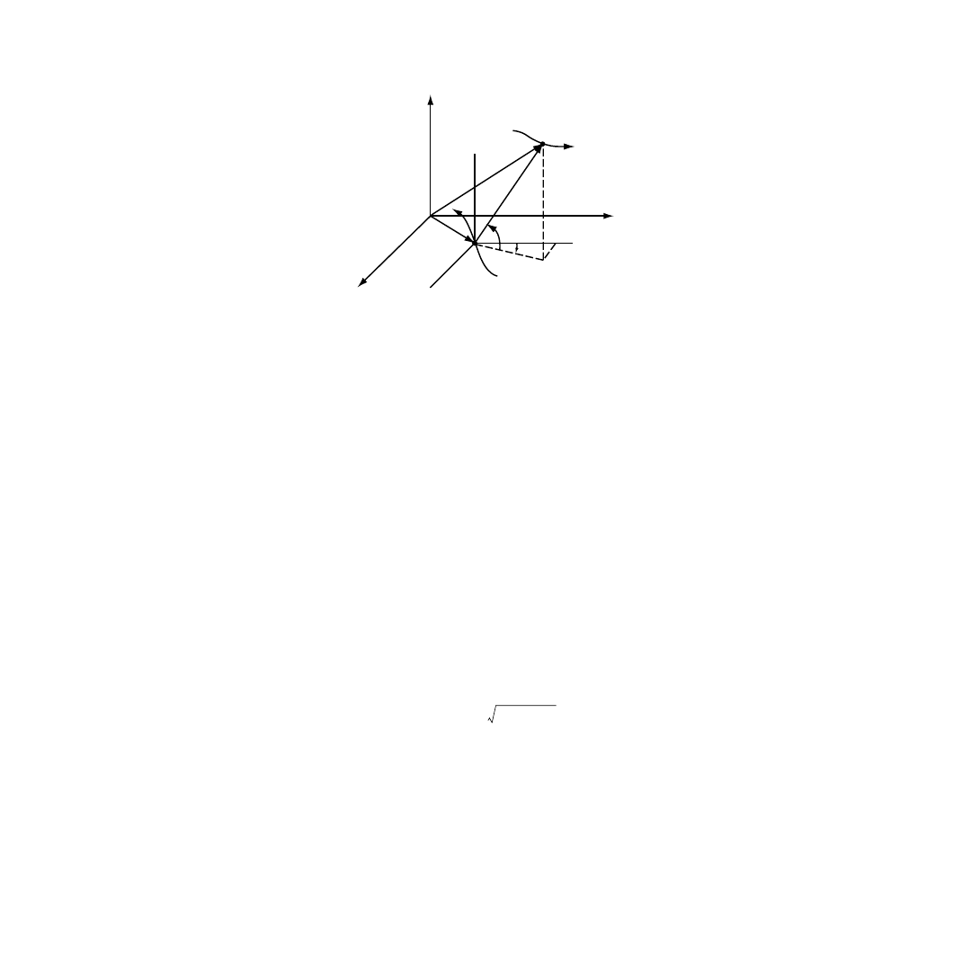
be composed of various types as well. To give an example, let us consider the measurement type angles
and Doppler-shifted frequencies in the three-dimensional scenario illustrated in

Figure 9.1

. Here, the target

is moving along a trajectory r

(t). Let us assume that the target emits a signal of constant but unknown

frequency

. The observer moving along another trajectory r

(t) (assumed known) receives the signal

and tries to estimate the target state from passive measurements of the line-of-sight (LOS) angles

and/or of the Doppler-shifted frequency

. This leads to the three alternative measurement sets:

(9.1)

which are time histories of the LOS angles, the Doppler-shifted frequency, and the combined measure-
ment data, respectively.

In the absence of noise and interference, the angle and frequency measurements satisfy the non-

linear relations

(9.2)

(9.3)

(9.4)

whereas r(t) = r

(t) – r

(t) = (r

(t), r

(t))

is the target position relative to the observer, r = |r| is

its norm, and c is the signal velocity.

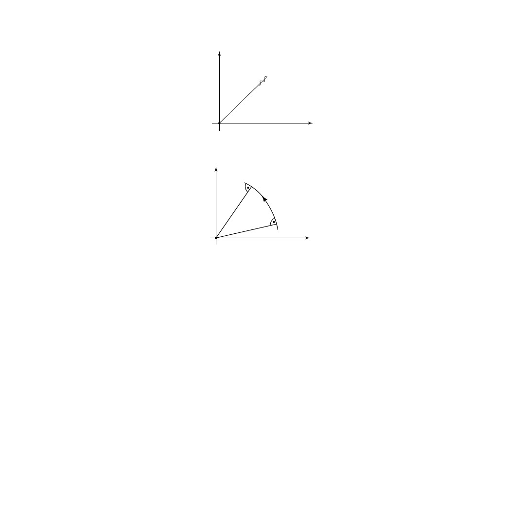
The estimation problem and its specific features change with the measurement set. There are target-

observer scenarios in which the sensitivities of the measurement Equations 9.2 to 9.4 may be quite
different. For example, whereas the orientation of the relative velocity has a strong effect on frequency,
the angles are not affected. That means that maneuvers may lead to a large variation in frequency, while
the angle variation is small and vice versa. Simple examples are weaving and spherical relative motions,
respectively, as illustrated in

Figures 9.2

and

9.3

for two-dimensional motions.

FIGURE 9.1

OBSERVER

TARGET

( ) φ

( )

{

} ν

( )

{

} β

( ) φ

( ) ν

( )

{

}

( )

arctan

( )

-----------

( )

arctan

( )

---------------------------------

( )

r˙ t

( )

r t

( )

⋅

cr t

( )

-----------------------

–









r˙ t

( )

---------

–









r˙

On the other hand, the different formulas may lead to measurement sets with qualitatively different

information content. For example, in a straight-line collision course, the angle measurement set provides
angle information only, and no information on closing velocity is contained. In contrast, the frequency
measurement set provides closing velocity information only (

assumed known), whereas angle infor-

mation is not contained. The qualitatively different information content leads to differently oriented
estimation error ellipsoids. From this, a significant gain in estimation accuracy may result when the
combined set of angle and frequency measurements is processed. This has been verified and discussed
in detail in the stationary target case,

for example.

Other significant differences resulting from the distinct measurement sets in Equation 9.1 will become

apparent in Section 9.2.2.

9.2.2 Observability

As indicated, a basic requirement for passive state estimation is the existence of a unique tracking solution.
This leads to the question of observability.

3–11

We shall say that the target state r

(t) is observable over

the time interval [t

, t

] if, and only if, it is uniquely determined by the measurements taken in that

interval. Otherwise, it is considered unobservable. The ensuing discussion covers the three specified
measurement sets in Equation 9.1. Since observability characteristics can be discerned under ideal
conditions, only the noise-free measurements Equations 9.2 to 9.4 need to be considered.

To understand the observability problem emanating from the measurement sets in Equation 9.1 in

full detail, it is important to know the transformations that leave the target trajectories compatible with
the measurements when no restrictions are imposed on the target motion. Observability analysis for a
particular target model then can be done in a systemic way by specializing the general set of compatible
trajectories to the model under consideration.

FIGURE 9.2

Weaving motion.

FIGURE 9.3

Spherical motion.

OBSERVER

TARGET

OBSERVER

TARGET

9.2.2.1 Fundamental Ambiguities

Provided that only the LOS angles are measured, it is obviously necessary and sufficient for trajectories
r

′

(t) to lead to the same measurement history as r

(t), if at all times the target lies on the LOS defined

by the direction of r(t). Thus,

(9.5)

where

(t) is an arbitrary scalar function greater than zero, i.e., both r

(t) and r

′

(t) have to be on the

same “side” of the observer in order for the LOS angles to be the same. Since

(t) is an arbitrary function,

the trajectory r

′

(t) may be of any shape.

If only frequencies are measured, the trajectories r

′

(t) and r

(t) trivially will lead to the same mea-

surement history if, and only if (cf. Equation 9.4),

(9.6)

where the prime signifies quantities associated with r

′

(t). Equation 9.6 may be rearranged as

–

ν′

–

ν′

). Integrating from t

to t and rearranging, we obtain

(9.7)

with

(9.8)

Conversely, it is easy to show that Equation 9.6 follows from Equation 9.7. Thus, a target trajectory r

′

(t)

cannot be distinguished from a trajectory r

(t) by frequency measurements in Equation 9.4, if, and only

if, the relative distance r

′

= |r

′

– r

| satisfies Equation 9.7. This is obviously true if, and only if, the

trajectories are of the form

(9.9)

where D(t) is an arbitrary orthogonal transformation.

If LOS angles and frequencies are measured, the compatible trajectories r

′

(t) necessarily must belong

to a common subset of the trajectories defined by Equations 9.5 and 9.9. Since none of the sets in
Equations 9.5 and 9.9 is a subset of the other, the intersection will remove some of the arbitrariness in
Equations 9.5 and 9.9. Evidently, by the additional angle measurements, the orthogonal transformation
in Equation 9.9 becomes the identity transformation, yielding trajectories which are contained in the set
defined by Equation 9.5. Therefore, in the case of angle and frequency measurements necessary and
sufficient for r

′

(t) to lead to the same measurement history as r

(t) is that r

′

(t) can be written as

(9.10)

with k + (a + c(1 – k)(t – t

))/(r(t) > 0).

Equations 9.5, 9.9, and 9.10 show that the true target trajectory is always embedded in a continuum

of compatible trajectories if no restrictions are imposed on the class of target motions. As an example,
let us consider Equation 9.10. Even if the signal frequency is supposed to be known, i.e.,

ν′

or k = 1,

′

( )

r t

( )

r˙
c

–









ν′

r˙

′

---

–









r˙

′

c 1

–

(

)

t t

–

(

)

ν′

-------

′

–

′

( )

D t

( )

c 1

–

(

)

t t

–

(

)

r t

( )

---------------------------------------------

r t

( )

′

( )

–

(

)

t t

–

(

)

r t

( )

---------------------------------------------

r t

( )

there is still a continuum of compatible trajectories parameterized by a = r

′

– r

which lead to the same

angle and frequency measurement history, i.e.,

(9.11)

The ambiguity is illustrated in

Figure 9.4

for a two-dimensional motion where, besides the true trajectory,

some compatible trajectories have been depicted within the observer’s coordinate system. According to
Equation 9.11, the compatible trajectories result from the true trajectory by a shift of the trajectory points
along the instantaneous LOS by an arbitrary but constant amount a.

The relation in Equation 9.11 constitutes a set of compatible trajectories if the measurement data are

composed of angle and frequency measurements. In case the measurement set, however, consists of angles
or frequencies only, Equations 9.5 and 9.9 introduce additional ambiguities into the curves of

Figure 9.4

Whereas Equation 9.5 removes the restriction on shape, Equation 9.9, of course, leaves the shape
unchanged, but the curves may be rotated, e.g., by an arbitrary angle.

The fundamental ambiguities of the target state exhibited in Equations 9.5, 9.9, and 9.10 in the class

of unrestricted target motions clearly demonstrate that in TMA the question for observability is of no
use unless specific target models are considered. Since the models impose restrictions on the analytical
behavior of the target state, the fundamental ambiguities change into specific ones. These can be resolved
in general by suitable observer maneuvers.

Note that in this way different target models may lead to completely different observability criteria.

Consequently, in case of model mismatch, there may be situations where the target state is observable within
the class of modeled motion, but is unobservable within the class of actual motion. The metric embedding
of the observed target trajectory in the unobservable ones via Equations 9.5, 9.9, and 9.10 then gives rise
to the fear that practical estimation algorithms may suggest convergence even in cases of divergence.

9.2.2.2 Nth-Order Dynamics Target

An illustrative example for a target model is the standard Nth-order dynamics model, i.e., the target
motion r

(t) can be described over the time interval [t

, t

] as a vector polynomial of degree N:

(9.12)

with

as the ith time derivative. Now, as a result of the model, r

′

(t) must also be a vector polynomial

of degree N. If this condition can only be fulfilled by r

′

(t)

≡

(t), then the set of compatible trajectories

shrinks to one single element and the state is observable, otherwise, it is not.

FIGURE 9.4

′

( )

r t

( )

---------

r t

( )

TRUE TRAJECTORY

OBSERVER

r(t)

( )

---------------

t t

–

(

)

∑

( )

To simplify the subsequent discussion, we introduce the class of vector polynomials

(9.13)

where A = (a

, …, a

) is a arbitrary 3

(N + 1) matrix of coefficients independent of t and t = (1, t – t

…, (t – t

)

. Obviously, r

(t)

∈

and

⊂

(n < N), as can be easily verified by a suitable choice of A.

For an illustration of how the method works, let us consider the measurement set {

(t),

(t)}. The

other measurement sets in Equation 9.1 are discussed in detail in Reference 9. The true target trajectory
is described by

(9.14)

Subtracting Equation 9.14 from Equation 9.5, the observer motion is eliminated: r

′

(t) – r

(t) =

(

(t) – 1)r(t). Since r

(t)

∈

and r

′

(t)

∈

, the difference also must be in

, i.e., (r

′

– r

)

∈

. So

′

– r

) must be of the form At as in Equation 9.13. From this, it follows that r(t) can be represented as

(9.15)

where

= (

– 1)

–1

. This is the necessary and sufficient condition for unobservability in the class of

Nth-order dynamics targets.

7–9

Examples

1. Obviously, the target cannot be observed from angle measurements in case of a constant LOS. This

can easily be verified from Equation 9.15 by selecting (t) = r(t) and A = (e

, 0

, …, 0

), where 0

is the three-dimensional null vector and e

is the constant unit vector in the direction of LOS.

2. For (t)

≡

1, Equation 9.15 reduces to r(t) = At, i.e., the target is unobservable, if r is a polynomial

of a degree less than or equal to N. From this, it follows that the target can be observed only if the
observer dynamics is of a higher degree than the target dynamics. This is reflected in the well-known
fact that a constant velocity target cannot be observed by a stationary or constant velocity observer.
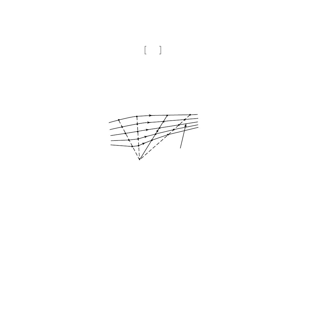
The condition of a higher observer dynamics degree, however, is only a necessary but not a sufficient
condition. The target may also be unobservable, even then when the observer motion is of a higher
degree than the target motion. This is true, e.g., when the higher order terms result in observer
displacements in the direction of the instantaneous LOS only, i.e., if the observer trajectory is of the
form r

(t) = A

t +

(t)r(t), where A

∈

and

(t)r(t) is the higher order terms observer motion.

Proof
Since r

= A

∈

, we have r = (A

– A

)t –

r. From this follows r = (1 +

)

–1

– A

)t, which is

of the form of Equation 9.15.

This proof is illustrated in

Figure 9.5

for the example of a constant velocity target.

9.3 Solution of the TMA Problem

9.3.1 Bearings-Only Tracking — A Typical TMA Problem

In the preceding section it has been shown that different types of measurement sets lead to estimation
problems different in nature. In this section, we develop the steps toward a solution of the problem.

Since the steps are the same irrespective of the type of measurement, we restrict the discussion to the

angles-only problem. Also, the three-dimensional problem is not particularly more enlightening than
the two-dimensional one. Therefore, for computational ease, we assume that the target and the observer
move in the (x,y)-plane of

Figure 9.1

. In doing so, the three-dimensional angles-only problem reduces

t t

–

(

)

= At

∑













( )

r t

( )

r t

( )

˜ t

( )

to the two-dimensional bearings-only problem. For simplicity reasons, we further assume that the target
moves along a straight line with constant velocity. Thus, the goal is to estimate the target position and
velocity through noisy bearing measurements and knowledge of the observer motion. Note that since
the bearings-only problem is a two-dimensional problem, the position vectors r

(t), r

(t), and r(t) denote

two-dimensional vectors in the (x,y)-plane throughout this section.

Let

(9.16)

be the Cartesian four-dimensional, position-velocity vector of the nonaccelerating target. Then a math-
ematical model of the target can be specified via the linear state equation

(9.17)

where

is the 2

2 null matrix, and I

is the 2

2 identity matrix. Integrating Equation 9.17, we

arrive at the solution

(9.18)

Herein is

(9.19)

the state transition matrix, which relates the state vector (Equation 9.16) at time t to the initial state
x

) at time t

FIGURE 9.5

Constant velocity target ambiguities in case of a constant velocity observer trajectory or its displace-

ment along instantaneous LOS.

OBSERVER

TRUE TARGET

( )

r˙

(

)

x˙

∅













∅

( )

t t

(

)

( )

t t

(

)

t t

–

(

)

∅













The bearing angle defined by the relation in Equation 9.2 is obviously a function of the unknown state

vector in Equation 9.16, i.e.,

(t)]. Viewed by the observer, the bearing, however, is noise corrupted.

Now, let a set of K bearing measurements

, i = 1, …, K, be collected at various times t

. Then in the

presence of additive errors n

, the measured bearings are given by

(9.20)

where

) and

)]. Since x

) =

, t

) for an arbitrary reference time t

(cf.

Equation 9.18), the angles

can be considered as functions of t

and of the constant state x

= x

Hence,

(9.21)

Identifying ,

, and n

with the components of vectors, Equation 9.20 can be organized in vector

form as

(9.22)

The measurement error n is a K-dimensional multivariate random vector with covariance matrix N =
E[(n – E[n])(n – E[n])

], where E[…] denotes the expected value.

In what follows, we assume that the measurement error n can be adequately described by a multivariate,

zero mean, normal probability distribution. Accordingly, the conditional density of

, given x

, is the

multivariate normal density

(9.23)

where det(2

N) denotes the determinant of 2

N. In addition, we assume that the measurements are

independent of each other and that the variances are independent of the measurement points, i.e.,

(9.24)

These are reasonable assumptions if the sampling frequency is not too high and if the measurement
points are much closer to each other than to the target.

The outlined two-dimensional, single observer, bearings-only problem has been the topic of much

research in the past.

12–26

The problem has been solved in detail in a variety of scenarios with different

approaches. For the numerical solutions, pertinent plots, and tables, we refer to the cited literature. A
discussion of these results is beyond the scope of this more tutorial chapter, which is confined to some
theoretical fundamentals only that will be discussed in the subsequent description of the solution steps.

9.3.2 Step 1 — Cramer-Rao Lower Bound

In judging an estimation problem, it is important to know the maximum estimation accuracy that can
be attained with the measurements. It is well known that the CRLB provides a powerful lower bound
on the estimation accuracy. Moreover, since it is a lower bound for any estimator, its parameter depen-
dence reveals characteristic features of the estimation problem. This and the fact that the optimal
performance bound is usually used as an evaluation basis for specific estimation algorithms are the very
reasons for the CR analysis to be a viable step in solving the TMA problem.

9.3.2.1 General Case

In its multi-dimensional form, the CR inequality states (see, e.g., References 27 and 28):

…

, ,

( )

[

]

( )

(

)

det 2

(

)

----------------------------

1
2

---

( )

–

[

]

–

( )

–

[

]

–













exp

Let a be an unknown parameter vector of dimension n and let (

) denote some unbiased estimate

of a based on the measurements

. Further, let C denote the covariance matrix of the estimation

error

∆

a = (

) – a and J the Fisher information matrix

(9.25)

where

∇

is the gradient with respect to a. Then the inequality

(9.26)

holds, meaning C – J

–1

is positive semidefinite.

The relation in Equation 9.26 is the multi-dimensional CR inequality, and J

–1

is the CRLB.

Geometrically, the covariance C can be visualized in the estimation error space by the concen-

tration ellipsoid

(9.27)

which has the volume

(9.28)

Herein V

is the volume of the n-dimensional unit hypersphere. In these terms, an equivalent formulation

of the CR inequality reads:

For any unbiased estimate of a, the concentration ellipsoid (Equation 9.27) lies outside or on the
bound ellipsoid (

Figure 9.6

) defined by

(9.29)

The size and orientation of the ellipsoid (Equation 9.29) can be best described in terms of the

eigenvalues and eigenvectors of the positive definite n

n matrix J. To this end, the eigenvalue problem

, (i = 1, …, n) has to be solved, where

, …,

are the eigenvalues of J and

, …,

are the

corresponding eigenvectors. The mutually orthogonal eigenvectors

coincide with the principal axes of

the bound ellipsoid, and the eigenvalues

establish the lengths of the semiaxes via

FIGURE 9.6

Geometrical visualization of the CRLB.

aˆ

∇

(

) ∇

(

)

(

)

[

]

–

≥

∆

–

∆

detC

∆

κ λ

⁄

a =

-1

a =

9.3.2.2 Bearings-Only Tracking

For bearings-only TMA considered in this section, we have a = x

, and the Fisher information

matrix is obtained from the conditional density in Equation 9.23. The gradient of the log-likelihood
function is

(9.30)

where

∂β

∂

is the Jacobian matrix of the vector function

). Inserting Equation 9.30 in Equation

9.25 and taking the expectation, the Fisher information matrix at reference time t

results in

(9.31)

which enters into the bearings-only tracking bound ellipsoid (cf. Equation 9.29)

(9.32)

The ith row of

∂β

∂

is calculated from Equation 9.21 by the chain rule

(9.33)

Denoting

= (cos

, – sin

, 0, 0) and considering that N is diagonal (cf. Equation 9.24), the matrix

in Equation 9.31 takes the particular form

(9.34)

Since

, t

) =

, t

)

, t

), it immediately follows that

(9.35)

Hence, if we know the information matrix at the reference time t

, we can calculate from it the information

matrix at an arbitrary time by a pre- and post-multiplication with the transition matrix

According to Equation 9.19, det

= 1. Consequently,

det J(t

) = det J(t

)

(9.36)

i.e., det J is invariant under shifts in the reference time. Since the inverse of det J is proportional to the
volume of the bound ellipsoid (Equation 9.32) (cf. Equation 9.28), we infer that time translations, of
course, may change the orientation and shape of the bound ellipsoid, while the total volume, however,
is preserved.

Due to the four-dimensional state parameter vector x

, the Fisher information matrix (Equation 9.31)

is a 4

4 matrix. The associated bound ellipsoid (Equation 9.32) is a hyperellipsoid in the four-

dimensional position-velocity space of mixed dimension and not amenable to direct geometrical inter-
pretation. Only the projections of the hyperellipsoid onto the position and velocity subspaces, respectively,
can be visualized and geometrically interpreted.

∇

(

)

∂

---------

–

( )

–

[

]

J t

( )

∂

---------

–

∂

---------

∆

J t

( )∆

∂

---------

x t

( )

[

]

∂

( )

∂

----------------------

∂

( )

∂

----------------

---

cos

sin

–

0 0

, ,

(

)Φ

(

)

J t

( )

-----

∑

(

)

----------

(

)

(

)

J t

( )Φ

(

)

J t

( )

Generally, the projection of the bound ellipsoid onto a subspace of the state vector corresponds to

the subspace estimation error bound when only the subspace components are classified as parameters
of real interest and all others as nuisance parameters of no practical interest.

Thus, the projection of

the hyperellipsoid onto the position subspace is the relevant estimation error bound of a location
system, in which the position components of the target are estimated irrespective of its velocity.
Obviously, the CRLB on this error is provided by the position space submatrix of J

–1

(cf. Equation

9.26), which can be written as

–1

(9.37)

where P denotes the projection operator P = (I

) that projects the four-dimensional position-velocity

space onto the two-dimensional position subspace. The corresponding estimation error bound (Equation
9.32) is an ellipse given by

(9.38)

The information matrix associated to the bound Equation 9.37 is its inverse. Naturally, the information

content is affected by the presence of the unknown velocity covariances. Their effect can be calculated
in an easy way from the partitioned form of Equation 9.31

(9.39)

where J

and J

are the 2

2 Fisher information matrices in the case of known velocity and known

position components, respectively, and J

is the 2

2 cross-term block matrix. Now, the difference J

–

(PJ

–1

)

–1

is the information loss due to the presence of the unknown velocity parameters. Since (PJ

–1

)

–1

is the Schur complement of J

the information loss is the positive definite matrix

(9.40)

A similar result holds for the projection of the hyperellipsoid onto the velocity subspace.

9.3.3 Step 2 — Estimation Algorithm

Good estimates of the target state are the ultimate goal in any TMA application. Consequently, powerful
estimation algorithms are a very important step in solving the TMA problem.

In this section, the single observer bearings-only tracking problem is considered. Unfortunately, this

type of estimation problem is not amenable to a simple solution. First, since observations and states are
not linearly related, conventional linear analysis cannot be applied. Second, the measurements provide
only directional information on the state and thereby introduce the question of system observability as
an important issue into the estimation problem. As discussed in Section 9.2.2, restrictions must be
imposed on the observer motion in order to warrant a unique tracking solution. In the considered
scenario, e.g., the observer must execute at least one maneuver. But even then, quite realistic target-
observer constellations often suffer from poor observability, in which cases TMA proves to be an ill-
conditioned estimation problem.

Numerous estimators have been devised for bearings-only TMA. From the implementation viewpoint,

the solutions can be loosely grouped into four categories: graphical methods, Kalman filters, explicit
methods, and search methods. The graphical solutions are earlier approaches proposed for use without
computers. Today, these methods are no longer of any practical value, and they are mentioned here only
for completeness reasons. More important are the numerical estimators. Here, a multitude of different

∅

∆

(

)

–

(

)

–

∆













–

(

)

–

algorithms exist. However, in the discussion to follow, we concentrate only on some prominent repre-
sentatives of each category. For a more complete list of algorithms, see, e.g., References 22 and 26.

• The Kalman filter solutions recursively update the target state estimates. Since the problem is

nonlinear, they are basically extended Kalman filters (EKF). Depending on the choice of coordi-
nates, linearizations are necessary for either the state or the measurement equation. Estimators of
this kind are

1. The Cartesian EKF:

12,13

The state equation is linear, whereas the measurement equation is

nonlinear. Although the solution can be very good, in many instances, however, it exhibits
divergence problems precipitated by a premature convergence of the covariance matrix prior
to the first observer maneuver.

2. The modified polar EKF (MPEKF):

14–16

The measurement equation is linear, but the state

equation is nonlinear. The filter is free from premature covariance convergence, since the
observable and the unobservable state components are automatically decoupled prior to the
first observer maneuver. The performance of the filter is good if initialized properly.

• The explicit methods provide solutions in explicit form as a function of the measurements.

The most well-known one is the pseudo-linear estimator (PLE).

17–23

In PLE, the nonlinear

measurement equation is replaced with an equation of pseudo-measurements that are derived
from the known observer state and the bearing measurements and are linearly related to the
target state. Thus, the method of linear least squares can be applied for the explicit solution.
Note that because of the linearity PLE may also be implemented in recursive form.

Geomet-

rically, the solution minimizes the sum of squared cross-range errors perpendicular to the
measured bearing. The PLE method avoids the instability problems of the Cartesian EKF.
However, it has not gained widespread acceptance because the estimates are biased whenever
noisy measurements are processed.

17,19

The bias can be severe, but modifications of PLE appear

to have limited that problem.

22,23

• The search methods are numerical optimization algorithms which iteratively improve the estimate.

They are basically batch methods using the entire measurement set at every iteration. A prominent
representative of this group is the MLE. The MLE is the best estimator,

20,22

but it is a computa-

tionally expensive solution.

From the performance aspect, MPEKF and MLE are both suitable candidates in a real-time system.

They will be discussed in more detail in Sections 9.3.3.1 and 9.3.3.2.

9.3.3.1 The Modified Polar Extended Kalman Filter

It is well known that the system equations often acquire entirely dissimilar properties when expressed in
different coordinate systems. In the same way, the performance of an estimator is affected by the choice
of coordinates.

The Cartesian formulation of the EKF, though appealing from the computational point of view, was

found to be unstable for bearings-only TMA. Therefore, research efforts have focused on alternative
coordinates that reduce the problems inherent in Cartesian EKF. Apparently, the premature covariance
convergence problem can be avoided by using coordinates whose observable and unobservable compo-
nents are decoupled in the filter equations prior to the first observer maneuver. Coordinates with these
attributes are, e.g., the modified polar (MP) coordinates.

The MP state vector is defined by

(9.41)

Herein the last three components are observable without an observer maneuver, while the first component
becomes observable only after a maneuver.

14,15

Differentiating Equation 9.41 with respect to time and

y t

( )

r t

( )

---------

( )

r˙ t

( )

r t

( )

---------

˙ t

( )









using the polar coordinate representation for the components of the Cartesian relative position vector r
= (rsin

, rcos

)

, we obtain the state equation in MP coordinates

(9.42)

where a

, a

are the Cartesian components of the observer acceleration

. The general solution of

the nonlinear differential Equation 9.42 can be expeditiously found by solving its Cartesian counterpart

(9.43)

of the relative state x = (r

)

and by making use of the one-to-one transformations

(9.44)

between the Cartesian and MP coordinate system.

The Cartesian state Equation 9.43 can be readily solved. The solution is a linear function of the initial

state x(t

), and it is given by

(9.45)

where

(9.46)

and t

denotes an arbitrary fixed value of time.

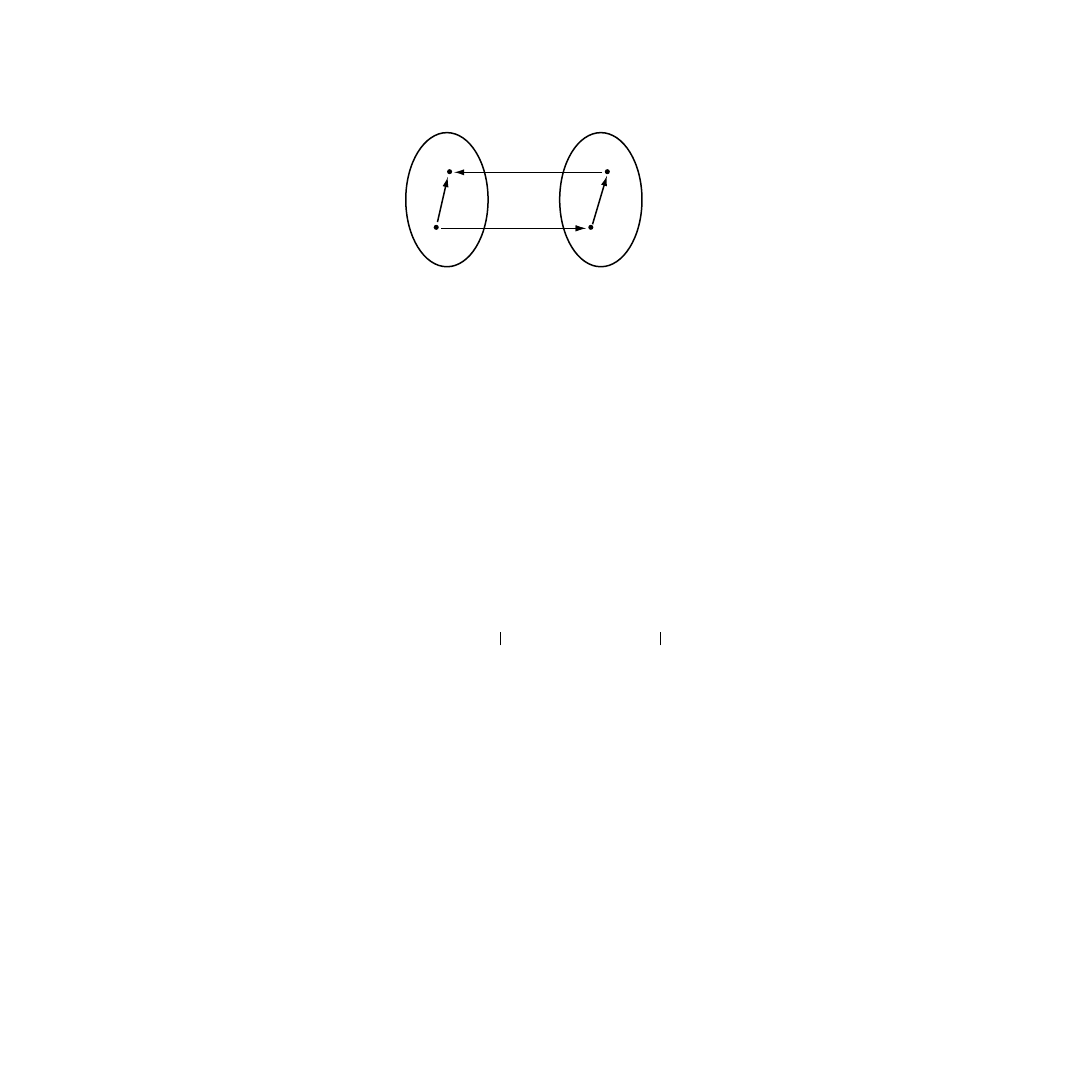
Using the relations in Equations 9.44 and 9.45, the solution of Equation 9.42 can obviously be written

in the form of three successive transformations. First, the initial MP state y(t

) is transformed via Equation

9.44 to its Cartesian counterpart x(t

), which then is linearly extrapolated via Equation 9.45. Finally, the

result x(t) is transformed via Equation 9.44 back to MP coordinates, giving the solution

(9.47)

which is a nonlinear function of y(t

). The solution scheme is illustrated in

Figure 9.7

Since

(t) is a component of the MP state vector (Equation 9.41), the nonlinear measurement Equation

9.20 becomes linear when expressed in MP coordinates, i.e.,

y˙

–

cos

sin

(

)

–

cos

sin

–

(

)

–

























r˙˙

x˙

∅













r˙˙













–

r˙

( )

x t

( )

t t

(

)

x t

( )

t t

(

)

–

L x t

( )

;

[

]

t t

(

)

–

(

)

( ) λ

∫

–

(

)

( ) λ

∫

( ) λ

∫

( ) λ

∫

















































y t

( )

f y t

( )

;

[

]

t t

(

)

y t

( )

[

]

t t

(

)

–

[

]

(9.48)

where

(9.49)

is the measurement matrix.

Equations 9.47 and 9.48 are the MP system equations in continuous form. From these, the discrete

time equations readily follow by assigning discrete values to t and t

. In the simplified index-only time

notation, we obtain

(9.50)

(9.51)

Expanding the nonlinear state Equation 9.50 in a Taylor series around the latest estimate y(k|k) and
neglecting higher than first-order terms, we arrive at the linearized state equation

(9.52)

where F

∂

f[y(k|k);t

k + 1

, t

∂

y(k|k) is the Jacobian of the vector function f. Straightforward application

of the Kalman filter to the linearized system Equations 9.52 and 9.51 results in the MPEKF. One cycle
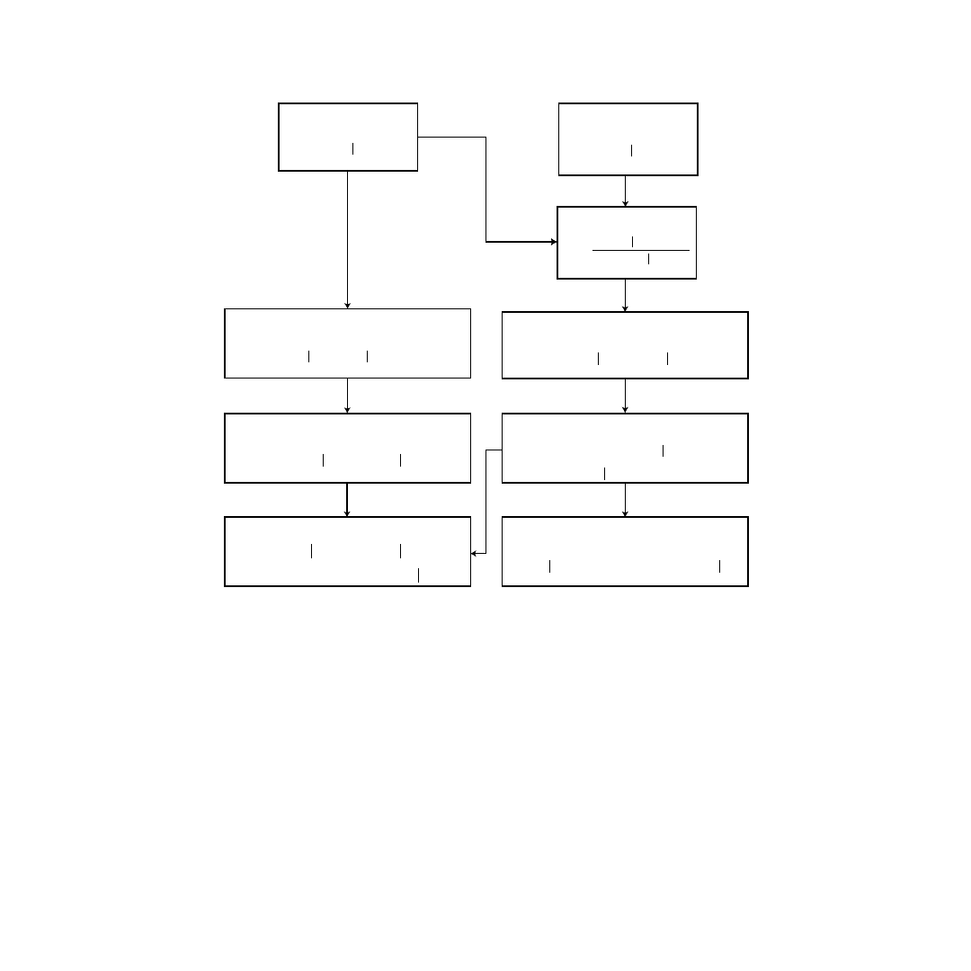
of the filter is presented in

Figure 9.8

Theoretical and experimental findings have conclusively shown that the performance of the MPEKF

is good provided that it is initialized by a proper choice of the initial state estimate y(0|0) and the initial
state covariance matrix P(0|0).

9.3.3.2 The Maximum Likelihood Estimator

Target tracking becomes increasingly difficult in a scenario of poor observability, for example, as in a
long-range scenario. The linearizations at each update in the recursive Kalman filter algorithms may then
lead to significant errors in this ill-conditioned estimation problem, whereas the MLE, as a batch algo-
rithm, avoids these linearization error effects.

For the problem specified in Section 9.3.1, the ML estimate is that value of x

which maximizes

Equation 9.23. Thus, the ML estimate minimizes the quadratic form

(9.53)

FIGURE 9.7

Solution scheme of the differential Equation 9.42.

MP coordinates

Cartesian coordinates

y (t)

x (t)

y (t

)

x (t

)

( )

Hy t

( )

n t

( )

0 1 0 0

, , ,

(

)

y k

(

)

f y k

( )

;

[

]

( )

Hy k

( )

n k

( )

y k

(

)

f y k k

(

)

;

[

]

y k

( )

y k k

(

)

–

[

]

Q x

( )

–

[

]

–

( )

–

[

]

-----

( )

–

[

]

∑

i.e., in case of a normal distribution the MLE and the least squares estimator with N

–1

as weight matrix

are identical.

Given a proper measurement set, the performance of the MLE is usually very good. In the single

observer bearings-only case, the MLE is known to be asymptotically efficient; but analytical closed-form
solutions do not exist. To find the minimum of Equation 9.53, a numerical iterative search algorithm is
needed. Consequently, application of MLE suffers from the same problems as the numerical algorithms.
Suitable optimization algorithms are e.g., the Gauss-Newton and the Levenberg-Marquardt method.

29,30

These methods are easy to implement, but to avoid a possibly large number of time consuming iteration
steps, good starting values are usually necessary.

9.3.4 Step 3 — Optimal Observer Motion

In TMA the estimation accuracy highly depends on the target-observer geometry. By changing the
geometry, estimation accuracy can increase or decrease, as the case may be. In an application, the target
motion is given and cannot be changed; but, if the observer is free to move, the target-observer geometry
can be changed by observer maneuvers. This leads to the final step in solving the TMA problem: Find
an optimal observer maneuver which creates a geometry that maximizes estimation accuracy.

FIGURE 9.8

Flowchart of MPEKF (one cycle).

state estimate at t

state covariance at t

y (k k)

P (k k)

measurement prediction

updated state estimate

state prediction covariance

filter gain

updated state covariance

Jacobian

state prediction

y(k + 1 k) = f[y (k k);t

]

P (k + 1 k) = F

P (k k) F

G (k + 1) = P (k + 1 k)H

[HP(k + 1 k)H

+ N(k + 1)]

-1

(k + 1 k) = Hy(k + 1 k)

P (k + 1 k + 1) = [I - G(k + 1)H]P(k + 1 k)

y(k + 1 k + 1) = y(k + 1 k)

+G(k + 1)[

(k + 1) -

(k + 1 k)]

∂

f [y(k k); t

k+1

, t

]

∂

y(k k)

From the discussion in Section 9.3.2, optimality is properly defined by the CRLB. Like the bound,

optimality criteria based upon CRLB are independent of the particular estimation algorithm. In the
literature, several criteria have been applied. One of them,

31,32

e.g., is maximizing

(9.54)

This is an intuitively appealing approach, since it minimizes the volume of the bound ellipsoid

(Equation 9.32) (cf. Equation 9.28). The determinant criterion (Equation 9.54) has, on the one hand,
the advantages that it is sensitive to the precision of all target state components and that it is independent
of the reference time (cf. Equation 9.36). On the other hand, however, it may be disadvantageous, because
using volume as a performance criterion may favor solutions with highly eccentric ellipsoids and with
large uncertainties in target state components of practical interest.

The eccentricity problem can be alleviated, e.g., by choosing an optimization criterion that minimizes

the trace of a weighted sum of the position and velocity lower bounds,

i.e.,

(9.55)

Herein P and Q are the projection operators onto the position and velocity space, respectively, and

are weight coefficients to decide whether position or velocity estimation is more important. The trace

of the position lower bound PJ

–1

is the sum of its eigenvalues, which according to Section 9.3.2.7 are

proportional to the square of the semiaxes of the bound ellipse (Equation 9.38). The same is true for the
trace of the velocity lower bound QJ

–1

and the bound ellipse in the velocity subspace. Therefore, the

optimality criterion (Equation 9.55) penalizes solutions with large semiaxes, and by this, it reduces the
possibly highly unbalanced estimation uncertainties resulting from the determinant criterion.

In a localization system the position components of the target state are of main interest. To improve

the estimation accuracy of these components, optimality criteria are needed that penalize the position
errors above all. To this end, criteria have been proposed that minimize the trace of the position
lower bound

(9.56)

or the range variance

22,32

(9.57)

respectively.

In finding the optimal observer trajectories for the various optimality criteria, Quasi-Newton optimi-

zation procedures

31,33,34

and optimal control theory

have been applied. The specific characteristics of

the solutions prove to be different for the individual criteria. For the details, we refer to the literature.
All solutions, however, involve a trade-off between increasing bearing rate and decreasing range.

9.4 Conclusion

Different types of measurements differ in their functional relation to the target state. As shown, this leads
to basically different estimation problems. The differences are reflected in the observability conditions
and the estimation accuracy as well. From this, we conclude that a measurement set consisting of different
measurement types will result in less restrictive observability conditions and in an improvement of
estimation accuracy. Depending on the qualitative differences of the estimates pertinent to the different
measurement types, the improvement may be substantial and may justify increased measurement equip-
ment complexity, all the more so as the computational complexity is not severely affected.

det

det J

trace

tr PJ

–

{

} α

tr QJ

–

{

}

plb

tr PJ

–

{

}

∂

---------

–

∂

---------









In the preceding section, the TMA problem is solved in three consecutive steps. The main step is the

development of a powerful algorithm that effectively estimates the target state from the noisy measure-
ments collected by the observer. The performance of the realized algorithm is usually assessed in a
simulation. In doing so, typical performance criteria of the estimator are unbiasedness and estimation
accuracy. Needed computer power is only a minor point in this context, due to the continually ongoing
rapid computer development. Whereas the question of unbiasedness can directly be answered by inspec-
tion, the question whether the estimation accuracy is good can only be conclusively answered by a
comparison with other estimators or even better by a comparison with an estimation error bound that
is independent of any specific estimation algorithm. A bound with this attribute is the CRLB. Its calcu-
lation is based on a theoretical measurement model, and because it is a function of the system parameters,
an analysis of its parametric dependences reveals characteristic features of the TMA problem under
consideration. Since the CRLB on the one hand gives a deep insight into the properties of the estimation
problem and on the other hand is used to evaluate particular estimators, the calculation and analysis of
the CRLB should always be the first step in solving the TMA problem.

In an application the user should always strive to get the maximum of attainable estimation accuracy.

Estimation accuracy can be influenced by the user first via the used algorithm and second, since it is a
function of the target-observer geometry, via observer motions as well. The improvement in estimation
accuracy via observer motions may be substantial even then, when the estimation accuracy of the used
estimator is generally very close to the CRLB. Therefore, if the observer is free to move, a final third step
is necessary in the TMA solution process. This step requires the solution of an optimal control problem,
in which the observer motion is controlled to achieve the maximum of attainable estimation accuracy.
Suitable optimality criteria in the solution of the problem can be derived, e.g., from the CRLB established
in the first solution step.

For a better understanding, the individual solution steps have exemplarily been discussed in the

relatively simple, constant target velocity, bearings-only TMA problem. Naturally, the complexity of the
solution steps increases with the complexity of the estimation problem. For example, the three-dimen-
sional angles-only TMA problem leads to far more complex equations than its two-dimensional bearings-
only counterpart. The same is true if the observer has no perfect knowledge of its own state or if the
target is allowed to maneuver. But, nevertheless, whatever cases are considered, the solution steps of the
pertinent TMA problem are always the same. They differ only in the level of complexity.

References

1. Constantine, J., Airborne passive emitter location (APEL), Proceedings of the Symposium on

Electronic Warfare Technology, Brussels, November 1993.

2. Becker, K., An efficient method of passive emitter location, IEEE Trans. Aerosp. Electron. Syst.,

AES-28, 1091–1004, 1992.

3. Nardone, S.C. and Aidala, V.J., Observability criteria for bearings-only target motion analysis, IEEE

Trans. Aerosp. Electron. Syst., AES-17, 162–166, 1981.

4. Shensa, M.J., On the uniqueness of Doppler tracking, J. Acoust. Soc. Am., 70, 1062–1064, 1981.
5. Hammel, S.E. and Aidala, V.J., Observability requirements for three-dimensional tracking via angle

measurements, IEEE Trans. Aerosp. Electron. Syst., AES-21, 200–207, 1985.

6. Payne, A.N., Observability conditions for angles-only tracking, in Proceedings of the 22nd Asilomar

Conference on Signals, Systems, and Computers, pp. 451–457, October 1988.

7. Fogel, E. and Gavish, M., Nth-order dynamics target observability from angle measurements, IEEE

Trans. Aerosp. Electron. Syst., AES-24, 305–308, 1988.

8. Becker, K., Simple linear theory approach to TMA observability, IEEE Trans. Aerosp. Electron. Syst.,

AES-29, 575–578, 1993.

9. Becker, K., A general approach to TMA observability from angle and frequency measurements,

IEEE Trans. Aerosp. Electron. Syst., AES-32, 487–494, 1996.

10. Jauffret, C. and Pillon, D., Observability in passive target motion analysis, IEEE Trans. Aerosp.

Electron. Syst., AES-32, 1290–1300, 1996.

11. Song, T.L., Observability of target tracking with bearings-only measurements, IEEE Trans. Aerosp.

Electron. Syst., AES-32, 1468–1472, 1996.

12. Kolb, R.C. and Hollister, F.H., Bearings-only target motion estimation, in Proceedings of the 1st

Asilomar Conference on Circuits and Systems, pp. 935–946, 1967.

13. Aidala, V.J., Kalman filter behavior in bearings-only tracking applications, IEEE Trans. Aerosp.

Electron. Syst., AES-15, 29–39, 1979.

14. Hoelzer, H.D., Johnson, G.W., and Cohen, A.O., Modified Polar Coordinates — The Key to Well

Behaved Bearings-Only Ranging, IBM Rep. 78-M19-0001A, IBM Shipboard and Defense Systems,
Manassas, VA, 1978.

15. Aidala, V.J. and Hammel, S.E., Utilization of modified polar coordinates for bearings-only tracking,

IEEE Trans. Automat. Control, AC-28, 283–294, 1983.

16. Van Huyssteen, D. and Farooq, M., Performance analysis of bearings-only tracking algorithm, in

SPIE Conference on Acquisition, Tracking, and Pointing XII, Orlando, FL, pp. 139–149, 1998.

17. Lindgren, A.G. and Gong, K.F., Position and velocity estimation via bearing observations, IEEE

Trans. Aerosp. Electron. Syst., AES-14, 564–577, 1978.

18. Lindgren, A.G. and Gong, K.F., Properties of a nonlinear estimator for determining position and

velocity from angle-of-arrival measurements, in Proceedings of the 14th Asilomar Conference on
Circuits, Systems, and Computers, pp. 394–401, November 1980.

19. Aidala, V.J. and Nardone, S.C., Biased estimation properties of the pseudolinear tracking filter,

IEEE Trans. Aerosp. Electron. Syst., AES-18, 432–441, 1982.

20. Nardone, S.C., Lindgren, A.G., and Gong, K.F., Fundamental properties and performance of conven-

tional bearings-only target motion analysis, IEEE Trans. Automat. Control, AC-29, 775–787, 1984.

21. Holst, J., A Note on a Least Squares Method for Bearings-Only Tracking, Tech. Rep. TFMS-3047,

Department of Math. Stat., Lund Institute of Technology, Sweden, 1988.

22. Holtsberg, A., A Statistical Analysis of Bearing-Only Tracking, Ph.D. dissertation, Department of

Math. Stat., Lund Institute of Technology, Sweden, 1992.

23. Holtsberg, A. and Holst, J., A nearly unbiased inherently stable bearings-only tracker, IEEE J.

Oceanic Eng., 18, 138–141, 1993.

24. Petridis, V., A method for bearings-only velocity and position estimation, IEEE Trans. Automat.

Control, AC-26, 488–493, 1981.

25. Pham, D.T., Some quick and efficient methods for bearings-only target motion analysis, IEEE

Trans. Signal Process., 41, 2737–2751, 1993.

26. Nardone, S.C. and Graham, M.L., A closed-form solution to bearings-only target motion analysis,

IEEE J. Oceanic Eng., 22, 168–178, 1997.

27. Van Trees, H.L., Detection, Estimation, and Modulation Theory, Part 1, Wiley, New York, 1968.
28. Scharf, L.L., Statistical Signal Processing, Addison Wesley, New York, 1991.
29. Gill, P.E., Murray, W., and Wright, M.H., Practical Optimization, Academic Press, New York, 1981.
30. Dennis, J.E. and Schnabel, R.B., Numerical Methods for Unconstrained Optimization and Nonlinear

Equations, Prentice-Hall, Englewood Cliffs, NJ, 1983.

31. Hammel, S.E., Optimal Observer Motion for Bearings-Only Localization and Tracking, Ph.D.

thesis, University of Rhode Island, Kingston.

32. Passerieux, J.M. and van Cappel, D., Optimal observer maneuver for bearings-only tracking, IEEE

Trans. Aerosp. Electron. Syst., AES-34, 777–788, 1998.

33. Helferty, J.P. and Mudgett, D.R., Optimal observer trajectories for bearings-only tracking by min-

imizing the trace of the Cramer-Rao lower bound, in Proceedings of the 32nd Conference on
Decision and Control, San Antonio, TX, pp. 936–939, December 1993.

34. Helferty, J.P., Mudgett, D.R., and Dzielski, J.E., Trajectory optimization for minimum range error

in bearings-only source localization, in OCEAN’93, Engineering in Harmony with Ocean Proceed-
ings, Victoria, BC, Canada, pp. 229–234, October 1993.

Document Outline

Advanced Signal Processing Handbook
- Contents
- Chapter 9: Target Motion Analysis (TMA)

Wyszukiwarka

Podobne podstrony:
(ebook pdf) Mathematics Statistical Signal Processing WLBIFTIJHHO6AMO5Z3SDWWHJDIBJQVMSGHGBTHI
1Introduction Signal Processing Haslerid 19014 (2)
Algorithm Collections for Digital Signal Processing Applications using Matlab E S Gopi
Algorithm Collections for Digital Signal Processing Applications using Matlab E S Gopi
Digital Signal Processing Teil 4
Advance 9PL Process Control
Digital Signal Processing Teil 1
Digital Signal Processing Teil 3
Digital Signal Processing Teil 2
2 Advanced X Sectional Results Using Paths to Post Process
2 Advanced X Sectional Results Using Paths to Post Process
W4 Proces wytwórczy oprogramowania
WEWNĘTRZNE PROCESY RZEŹBIĄCE ZIEMIE
Proces tworzenia oprogramowania
Proces pielęgnowania Dokumentacja procesu

więcej podobnych podstron