Johnny Lam report 238

Control of an Inverted Pendulum

Johnny Lam

Abstract. The balancing of an inverted pendulum by
moving a cart along a horizontal track is a classic problem
in the area of control. This paper will describe two methods
to swing a pendulum attached to a cart from an initial
downwards position to an upright position and maintain that
state. A nonlinear heuristic controller and an energy
controller have been implemented in order to swing the
pendulum to an upright position. After the pendulum is
swung up, a linear quadratic regulator state feedback
optimal controller has been implemented to maintain the
balanced state. The heuristic controller outputs a repetitive
signal at the appropriate moment and is finely tuned for the
specific experimental setup. The energy controller adds an
appropriate amount of energy into the pendulum system in
order to achieve a desired energy state. The optimal state
feedback controller is a stabilizing controller based on a
model linearized around the upright position and is effective
when the cart-pendulum system is near the balanced state.
The pendulum has been swung from the downwards
position to the upright position using both methods and the
experimental results are reported.

1. INTRODUCTION

The inverted pendulum system is a standard problem in the
area of control systems. They are often useful to
demonstrate concepts in linear control such as the
stabilization of unstable systems. Since the system is
inherently nonlinear, it has also been useful in illustrating
some of the ideas in nonlinear control. In this system, an
inverted pendulum is attached to a cart equipped with a
motor that drives it along a horizontal track. The user is
able to dictate the position and velocity of the cart through
the motor and the track restricts the cart to movement in the
horizontal direction. Sensors are attached to the cart and the
pivot in order to measure the cart position and pendulum
joint angle, respectively. Measurements are taken with a
quadrature encoder connected to a MultiQ-3 general
purpose data acquisition and control board.

Matlab/Simulink is used to implement the controller and
analyze data.

The inverted pendulum system inherently has two

equilibria, one of which is stable while the other is unstable.
The stable equilibrium corresponds to a state in which the
pendulum is pointing downwards. In the absence of any
control force, the system will naturally return to this state.
The stable equilibrium requires no control input to be
achieved and, thus, is uninteresting from a control
perspective. The unstable equilibrium corresponds to a state
in which the pendulum points strictly upwards and, thus,
requires a control force to maintain this position. The basic
control objective of the inverted pendulum problem is to
maintain the unstable equilibrium position when the
pendulum initially starts in an upright position. The control
objective for this project will focus on starting from the
stable equilibrium position (pendulum pointing down),
swinging it up to the unstable equilibrium position
(pendulum upright), and maintaining this state.

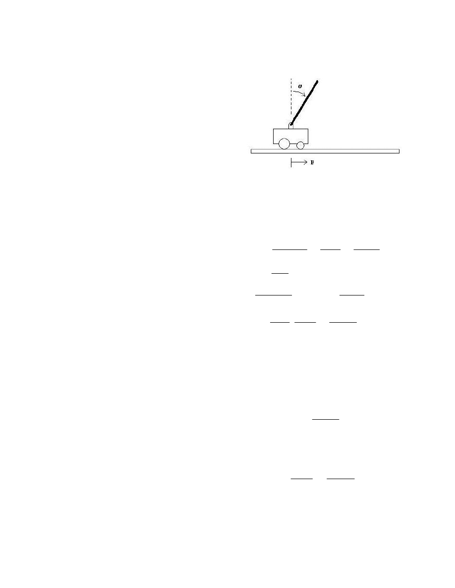
2. MODELLING

A schematic of the inverted pendulum is shown in Figure 1.

Figure 1. Inverted Pendulum Setup

A cart equipped with a motor provides horizontal motion of
the cart while cart position, p, and joint angle, θ,
measurements are taken via a quadrature encoder.

By applying the law of dynamics on the inverted

pendulum system, the equations of motion are:

( )

( ) ( )

( )

sin

cos

)

(

M -

−

⎟

⎟
⎠

⎞

⎜

⎜
⎝

⎛

(1)

( )

( ) ( )

( )

cos

sin

cos

sin

cos

⎟

⎟
⎠

⎞

⎜

⎜
⎝

⎛

−

⎟

⎟
⎠

⎞

⎜

⎜
⎝

⎛

)

L -

(2)

where m

is the cart mass, m

is the pendulum mass, I is the

rotational inertia, l is the half-length of the pendulum, R is
the motor armature resistance, r is the motor pinion radius,
K

is the motor torque constant, and K

is the gearbox ratio.

Also, for simplicity,

(3)

and note that the relationship between force, F, and voltage,
V, for the motor is:

−

. (4)

Let the state vector be defined as:

(5)

Finally, we linearize the system about the unstable
equilibrium (0 0 0 0)

. Note that θ = 0 corresponds to the

(

)

pendulum being in the upright position. The linearization of
the cart-pendulum system around the upright position is:

(6)

where

(7)

⎟⎟

⎠

⎞

⎜⎜

⎝

⎛

⎟

⎠

⎞

⎜

⎝

⎛

⎟⎟

⎠

⎞

⎜⎜

⎝

⎛

−

;

Finally, by substituting the parameter values that correspond
to the experimental setup:

(8)

.

This system will allow us to design a controller to balance
the inverted pendulum around the point of linearization.

STABILIZING CONTROLLER DESIGN

The controller design approach for this project is broken up
into two components. The first part involves the design of
an optimal state feedback controller for the linearized model
that will stabilize the pendulum around the upright position.
The second part involves the design of a controller that
swings the pendulum up to the unstable equilibrium. When
the pendulum approaches the linearized point, the control
will switch to the stabilizing controller which will balance
the pendulum around the upright position.

The state feedback controller responsible for

balancing the pendulum in the upright position is based on a

Linear Quadratic Regulator (LQR) design using the
linearized system. In a LQR design, the gain matrix K for a
linear state feedback control law u = -Kx is found by
minimizing a quadratic cost function of the form

, (9)

∫

∞

Ru(t)dt

u(t)

Qx(t)

x(t)

where Q and R are weighting parameters that penalize
certain states or control inputs.

The weighting parameters chosen in the design of

the optimal state feedback controller are:

⎟⎟

⎟

⎠

⎞

⎜⎜

⎜

⎝

⎛

−

⎟⎟

⎠

⎞

⎜⎜

⎝

⎛

−

⎟⎟

⎠

⎞

⎜⎜

⎝

⎛

−

10000

⎟⎟

⎟

⎠

⎞

⎜⎜

⎜

⎝

⎛

(10)

Based on this design, the controller gain matrix for the
linearized system is:

(

)

5668

6568

180

4448

0916

. (11)

By using this K and the control law u = -Kx, the system is
stabilized around the linearized point (pendulum upright).
Since this control law is based on the linearized system, the
state feedback optimal controller is only effective when the
pendulum is near the upright position.

4. STATE ESTIMATION

For the inverted pendulum experimental setup, not all the
state variables are available for measurement. In fact, only
the cart position, p, and the pendulum angle, θ, are directly
measured. This means that the cart velocity and the
pendulum angular velocity are not immediately available for
use in any control schemes beyond just stabilization. Thus,
an observer is relied upon to supply accurate estimations of
the states at all cart-pendulum positions.

A linear full state observer can be implemented

based on the linearized system derived earlier. This
observer is simple in design and provides accurate
estimation of all the states around the linearized point. The
observer is implemented by using a duplicate of the
linearized system dynamics and adding in a correction term
that is simply a gain on the error in the estimates. The
observer gain matrix is determined by an LQR design
similar to that used to determine the gain of the optimal state
feedback stabilizing controller. In this case, the weighting
parameters are chosen to be:

(12)

10000

⎟⎟

⎠

⎞

⎜⎜

⎝

⎛

⎟⎟

⎟

⎠

⎞

⎜⎜

⎜

⎝

⎛

Based on this design, the observer gain matrix is:

⎟⎟

⎟

⎠

⎞

⎜⎜

⎜

⎝

⎟⎟

⎠

⎞

⎜⎜

⎝

⎛

⎟⎟

⎟

⎠

⎞

⎜⎜

⎜

⎛

−

⎟⎟

⎟

⎞

⎜⎜

⎜

⎝

⎛

⎟⎟

⎟

⎞

⎜⎜

⎜

⎛

−

⎟⎟

⎟

⎠

⎞

⎜

⎛ p

⎝

⎠

⎝

⎜⎜

⎜

⎛

. (13)

⎟⎟

⎠

⎞

⎜⎜

⎝

⎛

−

0490

9999

0015

9999

Since the linear full state observer is based on the

linearized system, it is only effective in estimating the state
variables when the cart-pendulum system is near the upright
position. Thus, a low-pass filtered derivative is used to
estimate the two unmeasured states, cart velocity and
pendulum angular velocity, when the system is not close to
the unstable equilibrium. This method approximates the
cart velocity and pendulum angular velocity by using a
finite difference and then passing it through a low-pass
filter. The following filter is chosen for this estimation
method:

G(s)

. (14)

The problems with such a method are that it introduces
some delay and has a gain that is slightly less than one. The
state estimates obtained from the filtered derivative,
however, are reasonably accurate for the swing-up
controllers implemented in this paper.

SWING-UP CONTROLLER DESIGN

Two different control schemes were implemented to swing
the pendulum from the downwards position to the upright
position. The first is a heuristic controller that provides a
constant voltage in the appropriate direction and, thus,
drives the cart back and forth along the track repeatedly. It
will repeat this action until the pendulum is close enough to
the upright position such that the stabilizing controller can
be triggered to maintain this balanced state. The second
scheme is an energy controller that regulates the amount of
energy in the pendulum. This controller inputs energy into
the cart-pendulum system until it attains the energy state
that corresponds to the pendulum in the upright position.
Similar to the heuristic control method, the energy control
method will also switch to the stabilizing controller when
the pendulum is close to the upright position. The switch
that triggers the stabilizing controller in both cases is
activated when the pendulum is within 5° of the upright
position and the angular velocity is slower than 2.5 radians
per second.

Heuristic Controller
The heuristic controller is a logic-based control design that
determines the direction and the moment in time the cart
should move depending on the state of the system. A
specific voltage gain is applied to the cart motor based on
results from repeated experimentation. This controller will
make the cart drive forward or back whenever the pendulum
crosses the downwards position and depending on the
direction that the pendulum is swinging when it reaches the
downwards position.

The logic-based control design is completely

dependent on the pendulum angle, one of the available
measured state variables. The control scheme will change
the direction of the cart movement whenever the pendulum

angle crosses the downwards position. Since this control
design is based solely on the pendulum angle, the
downwards position is the optimal moment in time to add
energy to the pendulum by moving the cart in the
appropriate direction. The direction the cart moves is the
opposite sign of the pendulum angle immediately after it
crosses the downwards position. When the direction of the
cart movement is determined, a constant voltage gain is
applied to the cart motor in that same direction until the
pendulum returns to the downwards position. This control
scheme will effectively move the cart back and forth along
the track repeatedly until the pendulum swings close enough
to the upright position.

It is important to note that the nature of this control

scheme is that the same cart movement is applied regardless
of whether the pendulum is above or below the horizontal
axis (since the sign of the pendulum angle remains the
same). The nature of the cart-pendulum system, however, is
that the same cart movement that once added energy to the
pendulum while it was below the horizontal axis now
actually takes away energy from the pendulum. Eventually,
the pendulum will reach a point where it can add no more
energy to the pendulum system but it has yet to build
enough energy to reach the upright position. To avoid this
phenomenon, a switch has been implemented that changes
the voltage input to the cart motor to 0 when the pendulum
is 135° from the downwards position. As a result, the cart
will not move to take energy away from the pendulum
system when the pendulum is higher than 135°. This will
allow the pendulum to simply return to the downwards
position without losing anymore energy. When the
pendulum crosses the downwards position again, the logic-
based controller will be able to add more energy to the
pendulum until it eventually approaches the upright
position.

The voltage gain of this control scheme is

determined by repeated experimentation. There is a direct
correlation between the time it takes to swing the pendulum
to its upright position and the magnitude of the voltage gain.
A gain that is too high, though, may make the pendulum
approach the upright position with too high a velocity and,
thus, the stabilizing controller will be unable to balance the
pendulum. On the other hand, a gain too low may not
provide enough energy to the pendulum so that it can reach
the upright position. Also, the reliability of the controller in
performing the task varies depending on the gain selected.
Thus, repeated experimentation is required to finely tune the
gain so that the pendulum approaches the upright position
with just the right amount of velocity and in a reasonable
amount of time with a high success rate.

Energy Controller
The swinging up of a pendulum from the downwards
position can also be accomplished by controlling the amount
of energy in the system. The energy in the pendulum
system can be driven to a desired value through the use of
feedback control. By adding in enough energy such that its
value corresponds to the upright position, the pendulum can
be swung up to its unstable equilibrium. When the
pendulum is close to the upright position, the stabilizing
controller designed earlier can be triggered to catch the
pendulum and balance it around the unstable equilibrium.

The system is defined such that the energy, E, is

zero in the upright position. The energy of the pendulum
can be written as

⎟

⎟
⎠

⎞

⎜

⎜
⎝

⎛

−

⎟⎟

⎠

⎞

⎜⎜

⎝

⎛

cos

(15)

where

(16)

and m

is the mass of the pendulum, l is the half-length of

the pendulum, g is the acceleration of gravity, and I is the
rotational inertia. Thus, the energy in the pendulum is a
function of the pendulum angle and the pendulum angular
velocity. Note also that the energy corresponding to the
pendulum in the downwards position is -2m

gl. The goal of

the control scheme is to add energy into the system until the
value corresponds to the pendulum in the upright position.

The control law implemented to achieve the

desired energy is

(17)

(

)

(

)

(

cos

sign

sat

−

)

where k is a design parameter and E

is the desired energy

level. The control output, a, is the acceleration of the pivot
which can be translated to a voltage input to the cart motor
by using equation (4) and the fact that:

(18)

≈

for the system. In this control scheme, the sat

function is

defined as the value for which the voltage supplied to the
cart saturates. This controller essentially uses pendulum
angle and pendulum angular velocity to determine the
direction the cart should move at any point in time. A
proportional controller that scales with the amount of energy
still required to achieve the desired energy state dictates the
amount of voltage applied to the cart motor. The value of
the parameter V in sat

dictates the maximum amount of

control signal available and thus the maximum amount of
energy increase to the pendulum system. The value of k
determines how much the control favors using the
maximum control input to achieve the desired energy state.
This control is effective in increasing the energy of the
pendulum to a desired value. When used as a swing-up
control method, the desired value corresponds to the energy
of the pendulum in its upright position. This will allow the
switch to be triggered so that the stabilizing controller can
be used to catch the pendulum and balance it around the
unstable equilibrium point.

6. EXPERIMENTAL RESULTS

Results were gathered from the implementation of both
swing-up control methods. Data were collected from
experimental runs where each control scheme swings up the
pendulum from an initially downwards position to an

upright position and balances the pendulum around the
unstable equilibrium point.

The heuristic controller was finely tuned to swing

the pendulum by applying a constant voltage of 3.26 V.
Repeated experimentation with this voltage gain showed
that this controller was successful in swinging the pendulum
to an upright position for the stabilizing controller to
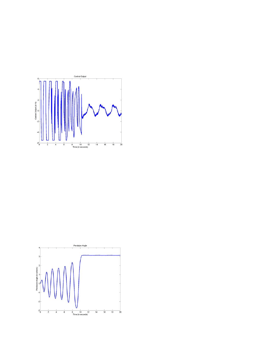
maintain the balanced state about 75% of the time. A plot
of the controller output during an experimental run for the
heuristic controller is shown in Figure 2.

Figure 2. Plot of Control Output for the Heuristic Controller

It is important to note that the swing-up controller

takes approximately 12.5 seconds to reach the upright
position. The point at which the stabilizing controller
catches the pendulum in the upright position is clearly
displayed in the plot. Also, the control output to the cart
motor alternates between 3.26 V and -3.26 V as determined
by pendulum angle. At a little under 7 seconds, the control
output also begins to output 0 V at small stretches of time
since the pendulum angle is beyond 135° from the
downwards position. Thus, it takes about another 5.5
seconds for the pendulum to get from beyond 135° from the
downwards position to within 5° of the upright position.

The corresponding plot of the pendulum angle is

shown in Figure 3. Each swing increases the pendulum
angle slightly until the pendulum is close to its unstable
equilibrium. The controller takes about 13 swings before
the pendulum is close enough to the upright position for the
stabilizing controller to catch it. The point in which the
stabilizing controller is activated is discernible from the
plot. Also, once activated, the pendulum angle remains
fairly constant around the balanced position.

Figure 3. Plot of the Pendulum Angle for the Heuristic Controller

The energy controller is implemented with the

design parameter, k, chosen to be 6.5. Also, as a result of
the friction in the cart-pendulum system and the
approximation made in equation (18), the desired energy
was offset to a value slightly higher than 0. The appropriate
offset can be determined through experimentation. In these
experiments, the offset is raised to E

= 0.70. Repeated

experimentation on the energy controller showed that this
controller was reliable at least 90% of the time. A plot of
the controller output during an experimental run using the
energy controller is shown in Figure 4.

Figure 4. Plot of the Control Output for the Energy Controller

It is important to note that the energy control takes

approximately 10 seconds to reach the upright position. The
control output initially alternates between 5.5 V and -5.5 V
since it attempts to increase the energy of the system as
quickly as it possibly can by using its maximum control
output (in this case, the saturation is defined to be at 5.5 V).
When the pendulum is close to the upright position, the
control output starts to decrease in magnitude since the
control output is based on the difference between the energy
of the system and the desired value. As with the heuristic
controller, the point at which the stabilizing controller is
activated is clearly discernible on the plot.

The corresponding plot of the pendulum angle for

the energy controller is shown in Figure 5. Note that with
each swing the pendulum angle is increased slightly. This
controller takes about 12 swings before the pendulum is

Figure 5. Plot of the Pendulum Angle for the Energy Controller

close to the upright position. It is easy to see that the
stabilizing controller is able to catch the pendulum and
balance it once the energy controller successfully swings the
pendulum to the upright position.

7. CONCLUSIONS

Two swing-up control schemes have been implemented that
will switch to a stabilizing controller when the pendulum is
near the upright position in order to balance the pendulum.
Both controllers are capable of successfully swinging a
pendulum from an initially downwards position to the
upright position and balancing the pendulum around that
point. The energy control happens to be more robust and
reliable than the heuristic controller in successfully
swinging the pendulum to the upright position. As the data
indicates, the energy controller is also slightly faster than
the heuristic controller implemented. Another advantage in
the energy controller is that it is capable of reaching the
upright position even if it runs out of track length and
begins to run into the walls at the end of the track. The
heuristic controller implemented in this paper, on the other
hand, will immediately fail once the cart hits the end of the
track. Both swing-up methods still require multiple swings
to reach the upright position and also require a stabilizing
controller to catch the pendulum in the upright position.
Overall, it is seen that the energy controller is more
convenient to swing up a pendulum to its unstable
equilibrium than the heuristic controller. It has been shown,
however, that both controllers can be effective in swinging a
pendulum to the upright position from the downwards
position.

8. REFERNCES

Astrom, K.J. and K. Furuta, “Swinging up a Pendulum by
Energy Control”, Automatica, Vol. 36, 2000

Smith, R. S, ECE 147b/ECE 238 Course Webpages,
http://www.ccec.ece.ucsb.edu/people/smith/

Eker, J, and K.J. Astrom, “A Nonlinear Observer for the
Inverted Pendulum”, 8th IEEE Conference on Control
Application, 1996

Chung, C.C. and J. Hauser, “Nonlinear Control of a
Swinging Pendulum”, Automatica, Vol. 31, 1995

Wyszukiwarka

Podobne podstrony:
PNADD523 USAID SARi Report id 3 Nieznany
238
Mądrzycki Deformacje w spostrzeganiu ludzi str 1 238
Ludzie najsłabsi i najbardziej potrzebujący w życiu społeczeństwa, Konferencje, audycje, reportaże,
REPORTAŻ (1), anestezjologia i intensywna terapia
Reportaż
Raport FOCP Fractions Report Fractions Final
reported speech
Reportaże telewizyjne
daily technical report 2012 10 03
Mazowieckie Studia Humanistyczne r2000 t6 n1 2 s236 238
MN 238 revII
O 238 1
Hydrostatics reportzaj
tab lam, Akademia Morska -materiały mechaniczne, szkoła, Mega Szkoła, PODSTAWY KON, Program do oblic

więcej podobnych podstron