
Non-Associative Local Lie Groups
Peter J. Olver
†
School of Mathematics
University of Minnesota
Minneapolis, MN 55455
olver@ima.umn.edu
Abstract.
A general method for constructing local Lie groups which are not con-
tained in any global Lie group is described. These examples fail to satisfy the global
associativity axiom which, by a theorem of Mal’cev, is necessary and sufficient for glob-
alizability. Furthermore, we prove that every local Lie group can be characterized by
such a covering construction, thereby generalizing Cartan’s global version of the Third
Fundamental Theorem of Lie.
1.
Introduction.
In Sophus Lie’s time, all Lie groups
‡
were local. The group was identified with an
open subset of Euclidean space, the group multiplication and inversion operations only
being defined for elements sufficiently near the identity. The global theory had to await
†
Supported in part by NSF Grants DMS 92–04192 and 95–00931.
‡
See [
4
; pp. 410–429] for a short historical survey of Lie group theory. Hofmann, [
11
], argues
that Lie’s investigations were more along the lines of a local semigroup theory, which had its
origins in a paper of Abel, [
1
]. In recent times, topological and Lie semigroups have become an
important area of research in their own right; see, for example, the book [
13
] and the papers in
[
14
], [
15
].
July 1, 2003
1

the proper abstract definition of manifold, and was finally codified in the work of ´
Elie
Cartan in the 1920’s. The question then arose as to whether every local Lie group was
contained in a global Lie group. This was answered affirmatively in the small by Cartan,
[6], who showed that every local Lie group contains a neighborhood of the identity which
is homeomorphic to a neighborhood of the identity of a global Lie group; see also [28;
Theorem 84]. Cartan’s result provides a global version Lie’s Third Fundamental Theorem
— every Lie algebra is the Lie algebra for a global Lie group. Indeed, the additional
conditions that the Lie group be connected and simply connected are enough to uniquely
specify it; any other connected global Lie group having the given Lie algebra is a quotient
of this “maximal” Lie group by a discrete normal subgroup.
The global counterpart to Cartan’s result is, however, not true. Not every local Lie
group is contained in a global Lie group. The problem of globalizability of local topological
groups was investigated in the 1930’s by P.A. Smith, [33], [34], and by Mal’cev, [19],
who pointed out the crucial connection between associativity and globalizability. Mal’cev
proved that a necessary and sufficient condition for the existence of a global topological
group containing a given local group is that it satisfy a certain “global” associativity
hypothesis — see Definition 4 below. Their work was continued by, among others, Van
Est, [35], Douady, [9], and, more recently, Plaut, [27], in connection with the study of
local groups of isometries, metric convergence, and pinching, cf. [26]. However, these
authors have tended to emphasize the infinite-dimensional version of Lie’s Third Theorem,
and all the examples of non-globalizable Lie groups appearing in their work are infinite-
dimensional topological groups. Less well investigated, but also of interest is the finite-
dimensional framework that forms the subject of this paper. A paper of Jacoby, [17],
stated some globalizability theorems for finite-dimensional local groups, but his proofs are
flawed. Indeed, the examples to be presented are readily seen to provide counterexamples
to Jacoby’s main globalizability theorem.
In this paper we describe a simple technique for constructing large families of examples
of non-globalizable local Lie groups, and prove that every local Lie group is contained in
one of these examples. The basic method is to start with a Lie group G, and let S ⊂ G be
an arbitrary closed subset not containing the identity element of G. It is not hard to see
that any covering manifold π: L → G \ S can be endowed with the structure of a local Lie
group which, in many instances, cannot be contained in any global Lie group. (A similar
construction appears in [2; p. 388].) Indeed, if, as usually happens, the resulting local Lie
group does not satisfy the global associativity axiom, Mal’cev’s Theorem implies that it
cannot be globalized. This paper includes a rather detailed analysis of the very simplest
example of this general construction, when G =
R
2
is the two-dimensional abelian Lie
group and S is a single point. However, the reader can readily see how these particular
constructions can be generalized.
Thus, the results in this paper provide an interesting counterpoint to the infinite
dimensional examples of Mal’cev, Van Est and Douady, leading to a wide class of finite
dimensional local Lie groups, which, by the globalizability theorem of Cartan, are locally
isomorphic to a neighborhood of the identity of a global Lie group, but which are not
themselves embeddable into any global Lie group. Thus, in analogy with the tripartite
division of the theory of Lie semigroups proposed in [12], the theory of finite-dimensional
2

Lie groups also divides into three parts — the infinitesimal theory, the local theory, and the
global theory. The present paper shows that the local theory is not a simple corollary of
the global theory of Lie groups, but has its own set of interesting and delicate geometrical
structures. Furthermore, our examples can be viewed as particular instances of non-
associative local group actions on manifolds — we just view the group acting on itself by left
multiplication — and can thus serve as useful test cases for the commonly misunderstood
role played by associativity in the analysis of local transformation groups. See Mostow,
[22], and Palais, [25], for results on globalizing local transformation group actions.
This work arose during the course of writing the book [24], when I was attempting
to establish a global version of the local equivalence results found by Cartan’s method
of equivalence, [7], [10]. The equivalence method, which (in the cases relevant to our
constructions) is based on the Frobenius Theorem, cf. [24; Chapter 14], [36], governing
the existence of solutions to certain involutive systems of partial differential equations,
can, in fact be employed to prove that these examples are the most general possible: every
local Lie group is a generalized covering, in the sense of Definition 16, of an open subset
of a global Lie group, leading to a complete characterization of the most general possible
local Lie group. See Theorem 21 for a precise statement of this result. In the final section,
we revisit Mal’cev’s Theorem, adapting and fleshing out the proof to show that a local Lie
group can be globalized if and only if it satisfies the global associativity condition.
2.
Local and Global Lie Groups.
We begin by formalizing the definitions of local and global Lie groups. For simplicity
we work in the smooth category, although results of Lie, [18; p. 366], and Schur, [32],
could be used to significantly relax our differentiability hypotheses. To avoid constant
repetition, we assume the blanket hypothesis that all groups and manifolds are assumed
to be connected. We begin with the standard definition of a Lie group.
Definition 1.
A global Lie group is a group G which also carries the structure of a
smooth manifold so that the operations of group multiplication
µ: G × G −→ G,
µ(g, h) = g · h,
g, h ∈ G
and inversion
ι: G −→ G,
ι(g) = g
−1
,
g ∈ G
are smooth, globally defined maps.
While the definition of a global Lie group is standard, the precise definition of a local
Lie group varies from author to author. The following one is slightly adapted from that
appearing in Pontryagin, [28; p. 83]; see also [4; §III.1.10], [23; Definition 1.20]. The group
multiplication is defined locally, meaning one of the multiplicands must be sufficiently close
to the identity element. The only difference between our definition and Pontryagin’s is that
we require the left and right inverses of a group element to both be defined, and the same,
whenever one or the other exists. This requirement could clearly be relaxed, without
appreciable complication.
3

Definition 2.
A smooth manifold L is called a local Lie group if there exists a) a
distinguished element e ∈ L, the identity element, b) a smooth product map µ: U → L
defined on an open subset ({e}×L)∪(L×{e}) ⊂ U ⊂ L×L, and c) a smooth inversion map
ι: V → L defined on an open subset e ∈ V ⊂ L such that V × ι(V) ⊂ U, and ι(V) × V ⊂ U,
all satisfying the following properties:
(i )
Identity:
µ(e, x) = x = µ(x, e) for all x ∈ L.
(ii )
Inverse:
µ(ι(x), x) = e = µ(x, ι(x)) for all x ∈ V.
(iii )
Associativity:
If (x, y), (y, z), (µ(x, y), z), and (x, µ(y, z)) all belong to U, then
µ(x, µ(y, z)) = µ(µ(x, y), z).
(1)
In the classical texts, L is assumed to be an open subset of Euclidean space, so
that the multiplication map µ(x, y) and the inversion map ι(x) are expressed in terms of
coordinates. However, allowing more general manifolds does not lead to any appreciable
change in either the methods or the results to be presented here.
Example 3.
The most basic example of a local Lie group is provided by any neigh-
borhood e ∈ N ⊂ G of the identity element in a global Lie group. Indeed, we set U to be
any open subset of N ×N such that ({e}×N)∪(N ×{e}) ⊂ U ⊂ (N ×N)∩µ
−1
(N ), and V
to be any open subset of N such that {e} ⊂ V ⊂ N ∩ι
−1
(N ) and (V ×ι(V))∪(ι(V)×V) ⊂ U.
The group multiplication µ and inversion ι on G then clearly restrict to define local group
multiplication and inversion maps on N .
Note that we can restrict the domains of definition of the local group multiplication
and inversion maps, leading to a family of “restricted” local group structures on L. Two
local group structures on the manifold L are locally homeomorphic if they have a common
restriction. In other words, the two local group structures on the same manifold L, defined
by (µ, U, ι, V), and (e
µ, e
U, eι, e
V), as per Definition 2, are locally homeomorphic provided
there exists open sets ({e} × L) ∪ (L × {e}) ⊂ b
U ⊂ U ∩ e
U, and e ∈ b
V ⊂ V ∩ e
V, on which the
two multiplications and inversions agree: µ| b
U = e
µ | b
U, ι|b
V = eι|b
V. Continuity then implies
that the two local group structure agree on the connected components (U ∩ e
U)
0
, (V ∩ e
V)
0
of
the intersections of their domains. However, the two local group structures need not agree
on the entire intersections U ∩ e
U, V ∩ e
V, which precludes the existence of a “maximal”
local group structure among the locally homeomorphic local group structures on a given
manifold L. By abuse of terminology, though, we shall refer to “the local Lie group L” with
the understanding that the local group structure may need to be appropriately restricted
if necessary.
There are several inequivalent ways of imposing the associativity requirement on a
local Lie group. The least restrictive is to require that it hold locally, meaning for triples
of group elements where two are sufficiently close to the identity; in other words, we require
(1) hold for (x, y, z) ∈ W, where
({e} × {e} × L) ∪ ({e} × L × {e}) ∪ (L × {e} × {e}) ⊂ W ⊂ Z ⊂ L × L × L,
is an open subset contained in the set
Z =
£
(1
1
× µ)
−1
U ∩ (L × U)
¤
∩
£
(1
1
× µ)
−1
U ∩ (L × U)
¤
⊂ L × L × L
4

of all (x, y, z) ∈ L × L × L for which both sides of equation (1) are defined. We shall
call such local groups locally associative. A similar condition appears in [17], [13; p. 542],
where one assumes the existence of an open set e ∈ Y ⊂ V such that Y × Y ⊂ U, and
requires (1) to hold whenever x, y, z, µ(x, y), µ(y, z) ∈ Y; this amounts to requiring local
associativity with W = (Y × Y × Y) ∩ (Y × µ
−1
(Y)) ∩ (µ
−1
(Y) × Y).
More restrictively, one can require that the associativity law hold for all triples of group
elements for which the required group products are defined. This means that W = Z, and
this is the version that I have chosen in Definition 2. Such local groups will be called
associative
for short.
There is a further generalized associative law that requires that associativity holds for
all possible iterated products. From now on, if S is any set, we let S
×n
= S ×· · ·×S denote
the n-fold Cartesian product of S with itself. Given an ordered n-tuple (x
1
, . . . , x
n
) ∈ L
×n
of local group elements, we can, provided they are defined, form a variety of n-fold products.
For example, the two sides of the associativity law (1) define the two possible three-fold
products. There are, potentially, five different products associated with an ordered four-
tuple (x
1
, x
2
, x
3
, x
4
) ∈ L
×4
, namely
µ(x
1
, µ(x
2
, µ(x
3
, x
4
))),
µ(x
1
, µ(µ(x
2
, x
3
), x
4
)),
µ(µ(x
1
, x
2
), µ(x
3
, x
4
)),
µ(µ(x
1
, µ(x
2
, x
3
)), x
4
),
µ(µ(µ(x
1
, x
2
), x
3
), x
4
).
Each possible n-fold product
†
of a given n-tuple is determined by an n-fold parenthesis
system, cf. [8; p. 53], or, equivalently, a complete, planar, rooted binary tree on whose
leaves are labeled by the x
i
’s, cf. [29; p. 4]. The precise number of possible n-fold products
of an ordered n-tuple of group elements (x
1
, . . . , x
n
) ∈ L
×n
, that is the number of possible
ways of introducing parentheses into the list, is therefore given by the Catalan number
C
n
=
1
n
µ
2n − 2
n − 1
¶
.
Definition 4.
A local Lie group is associative to order n if, for every 3 ≤ m ≤ n,
and every ordered m-tuple of group elements (x
1
, . . . , x
m
) ∈ L
×m
, all corresponding well-
defined m-fold products are equal. A local group is called globally associative if it is
associative to every order n ≥ 3.
Note that, in particular, the associativity assumption (iii ) in Definition 2 requires
that any local group be associative to order 3 (at least). Of course, for a global group,
associativity to order 3 automatically implies global associativity. The remarkable fact,
which is explicitly borne out by our examples, is that this is not the case for local groups.
Mal’cev’s theorem, [19], demonstrates that the condition of globally associativity is both
necessary and sufficient condition for a globally inversional local topological group to be
globalizable. Moreover, Mal’cev exhibits infinite-dimensional examples of globally inver-
sional topological groups which are associative to some fixed order n, but which fail to
satisfy the global associativity requirement, and hence cannot be contained in any global
group. Later, we shall see how to produce similar examples of local Lie groups that are
associative, but not globally associative.
†
Of course, not all of these products may be well defined.
5

Remark
: In an attempt to generalize the Gleason–Montgomery–Zippin Theorem, [21],
on topological groups and thereby solve Hilbert’s Fifth Problem
‡
for local Lie groups,
Jacoby, [17], claimed to prove that any locally Euclidean local group is contained in a
global Lie group. However, as pointed out by Plaut, [27], Jacoby did not appreciate the
significance of the global associativity assumption. Indeed, Jacoby’s Theorem 8, which
is stated without proof, essentially makes the false claim that local associativity implies
global associativity. Despite this initial flaw, it is likely that some of Jacoby’s results can
be recovered in a local or germ sense, or, alternatively, subject to an appropriate global
associativity assumption. Thus, it is probably correct to state that every locally Euclidean
local group is locally isomorphic to a neighborhood of the identity in a global Lie group.
Unfortunately, since the rest of Jacoby’s paper relies heavily on his incorrect Theorem 8,
the re-establishment of his results (in an appropriately amended form) would require a
significant effort. Such a project would not be without motivation — for instance, results
of Brown and Houston, [5], and Hofmann and Weiss, [16], that provide a positive solution
to Hilbert’s Fifth Problem for semigroups on manifolds, rely heavily on Jacoby’s results.
A map between local groups is a local group homomorphism provided it respects the
two multiplication and inversions where they are defined. Specifically:
Definition 5.
Let (L, µ, U, ι, V), and (e
L, e
µ, e
U, eι, e
V), be local Lie groups. A smooth
map Φ: L → e
L is called a local group homomorphism if
(i )
Φ × Φ( U) ⊂ e
U, Φ(V) ⊂ e
V, Φ(e) = ˜e,
(ii )
Φ(µ(g, h)) = e
µ(Φ(g), Φ(h)) for (g, h) ∈ U, and
(iii )
Φ(ι(g)) = eι(Φ(g)) for g ∈ V.
A local group homomorphism is called a homeomorphism if it is one-to-one, onto, with
smooth inverse.
Note that the image of a local group homeomorphism Φ: L → e
L effectively identifies L
as a restriction of the local group structure on e
L. We could further relax the requirement for
a local group homomorphism by only requiring that Φ respect the group multiplication and
inversion maps on suitably small open subsets. However, this completely local definition
can be subsumed in the present definition by utilizing a suitable restriction of the local
group structure on L.
The main focus of the present paper is to understand to what extent local groups
can be globalized, thereby identifying them as a neighborhood of the identity element in a
global Lie group of the same dimension. This will be formalized in the following definition.
Definition 6.
A local Lie group L is called globalizable if there exists a local group
homeomorphism Φ: L → N mapping L onto a neighborhood e ∈ N ⊂ G of the identity of
a global Lie group G.
‡
Hilbert’s fifth problem concerns the role of analyticity in general transformation groups, and
seeks to generalize the result of Lie, [
18
; p. 366], and Schur, [
32
]. The Gleason–Montgomery–
Zippin result only addresses the special case when a global Lie group acts on itself by right or left
multiplication.
6

Example 7.
Before proceeding further, it is useful to illustrate these concepts by a
simple example of a one-dimensional local Lie group, cf. [23; pp. 19–20]. Let M =
R. The
identity element will be e = 0. The formulas for the multiplication and inversion maps are
given by
µ(x, y) =
2xy − x − y
xy − 1
,
ι(x) =
x
2x − 1
.
(2)
First, we restrict the multiplication and inversion maps by defining L = {|x| <
1
2
}, and
using
U =
©
(x, y)
¯
¯ |x| <
1
2
, |y| <
1
2
, (3x − 2)(3y − 2) > 1, (5x − 2)(5y − 2) < 9
ª
⊂ L × L,
V = {−
1
2
< x <
1
4
} ⊂ L,
as the domains of definition of the multiplication and inversion maps. The reader can
straightforwardly verify that (2) does indeed define a globally associative, abelian, local
Lie group. Indeed, the local Lie group L can be globalized via an embedding into the
unique global, simply connected, one-dimensional Lie group G =
R. The map Φ: L → G
given by Φ(x) = x/(x − 1) satisfies Φ(µ(x, y)) = Φ(x) + Φ(y), and Φ(ι(x)) = −Φ(x) where
defined. Therefore Φ provides the desired local group homeomorphism mapping L to the
open interval N = {−1 < x <
1
3
} ⊂ G.
In fact, one can expand the domains of definition of the multiplication and inversion
maps in this example, but this leads to a curious phenomenon. The largest possible
domains that will still satisfy the local group axioms are b
U = { (x, y) | |xy| 6= 1 } ⊂ M × M
and b
V = { x | x 6=
1
2
, x 6= 1 } ⊂ M. However, in this situation, the group element 1 ∈ M
plays a strange role. We find µ(x, 1) = µ(1, x) = 1 for all x 6= 1, so that 1 defines an
“infinite group element”. Moreover, its “inverse” ι(1) = 1 can even be defined, although
the product of the two, µ(1, ι(1)), is not defined, and hence not equal to the identity. On
the other hand, the infinite group element is “inaccessible” since µ(x, y) = 1 if and only if
either x = 1 or y = 1. Note that we can complete M and G by adjoining a point at infinity,
realizing both as subsets of the projective line: M, G ⊂ RP
1
. The “group homomorphism”
Φ then extends to a global projective map of
RP
1
, thereby endowing the projective line
with the structure of a local Lie group with an infinite group element, containing a global
Lie group as a dense open subset.
Remark
: The latter construction in Example 7 is a special instance of a general com-
pactification process that can be applied to any noncompact, but locally compact group;
see [31] for details.
To avoid the pathologies caused by such infinite local group elements, we must impose
an additional invertibility assumption on the local group. The most common way to do
this, advocated in [19], [33], is to require that every group element have an inverse.
Definition 8.
A local Lie group L is called globally inversional if the inversion map
ι is defined everywhere, so that V = L.
For example, a local group {e} ⊂ N ⊂ G given by a neighborhood of the identity
element in a global Lie group will be globally inversional if and only if it satisfies the
7

symmetry restriction N = ι(N ). Bourbaki’s Lie group germs
†
, [4; §III.1.10], are the same
as globally inversional local Lie groups.
For our purposes, though, it is useful to weaken the rather severe global inversionality
assumption, without permitting the pathology of infinite group elements. One way to do
this is to require that the group multiplication map does not degenerate. More specifically,
define the left and right multiplication maps λ
x
, ρ
x
so that
λ
x
(y) = µ(x, y),
ρ
x
(y) = µ(y, x).
(3)
Definition 9.
A local Lie group L is called regular if, for each x ∈ L, the maps
λ
x
, ρ
x
defining left and right multiplication, (3), are diffeomorphisms on their respective
domains of definition.
Thus, in the local Lie group of Example 7, in order to retain regularity we must
throw away the infinite group element 1, since its left and right multiplication maps are
constant. A slightly more restrictive approach is to require that the group elements always
be expressible as products of invertible ones.
Definition 10.
An element x of a local Lie group L is called inversional if there
exist invertible elements x
1
, . . . , x
n
∈ V such that x equals an n-fold product of the x
i
’s.
A local Lie group L is called inversional if every x ∈ L is an inversional element.
The following result is straightforward; its converse, though, is not necessarily valid,
since the group might include additional components containing regular, but non-invertible
elements.
Proposition 11.
Every inversional local Lie group is regular.
The property of being inversional is related to the notion of connectivity of a local Lie
group. A global Lie group is connected if it forms a connected manifold. Although a first
glance this appears a reasonable definition in the case of a local Lie group, we have seen
that it permits inaccessible, non-regular group elements. Moreover, one of the principal
means of characterizing connected global Lie groups, which lies at the foundations of the
infinitesimal approach to Lie group analysis, [23], is no longer equivalent to the mere
connectivity of the manifold in the case of local groups.
Definition 12.
A subset U ⊂ L of a local Lie group L is said to generate L if
L =
S
∞
n
=1
U
(n)
. Here U
(n)
⊂ L denotes the subset consisting of all group elements x ∈ L
which can be written as a well-defined n-fold product of elements x
1
, . . . , x
n
∈ U.
For example, Definition 10 just says that a local Lie group is inversional if and only
if the domain V of the inversion map generates L. A key result in the theory of global
Lie groups states that any open neighborhood e ∈ U of the identity of a connected global
Lie group G generates the entire Lie group G, cf. [36; Proposition 3.18]. In particular,
†
The original French version [
3
; §III.1.10] uses the wonderful term “groupuscle” for a local
group or group germ.
8

choosing U to be contained in the image of the exponential map exp: g → G, we deduce that
every element of a connected Lie group can be written as a finite product of exponentials:
g = exp(v
1
)·. . .·exp(v
n
) for v
i
∈ g. Example 7 shows that, without additional assumptions,
this result is not necessarily valid for local Lie groups. We are therefore led to propose a
more restrictive notion of connectedness for a local Lie group.
Definition 13.
A local Lie group L is connected if
(i )
L is a connected manifold,
(ii )
the domains of definition of the multiplication and inversion maps are also connected,
(iii )
if U ⊂ L is any neighborhood of the identity, then U generates L.
Note that a connected global Lie group satisfies the revised Definition 13. In particular,
we can choose the generating neighborhood to be U = V, and thus deduce that connected
local Lie groups are automatically inversional:
Proposition 14.
Any connected local Lie group is inversional, and hence regular.
From now on, in accordance with our blanket hypothesis, all local Lie groups are be
assumed to be connected in the sense of Definition 13. Thus we replace a more general
local Lie group L, by the connected component L
0
containing the identity, which is defined
the largest open, connected, local Lie subgroup L
0
⊂ L.
3.
The Simplest Examples.
In order to understand our general construction of non-associative local Lie groups, it
is helpful to discuss the very simplest examples in some detail. The first example will be an
associative, regular, local Lie group which fails to be globally associative. This preliminary
example however, does not satisfy the global inversional property, and so we describe a
straightforward modification which is, in addition, globally inversional. The failure of the
global associativity axiom implies that neither example can be contained in any global Lie
group.
Let G =
R
2
denote the real, simply connected two-dimensional abelian Lie group. It
is convenient to identify G with the complex plane
C ' R
2
, and use complex notation for
the elements of G, even though we are considering G as a real Lie group. Let M = G\{−1}
denote the punctured plane. (Other than the fact that it is not the identity, there is nothing
special about choosing −1 as the distinguished point to omit.) Let L ' R
2
denote the
simply connected covering space of M , and let π: L → M denote the covering map. Note
that L can be identified with the Riemann surface associated with the function log(z + 1).
An element ˆ
z ∈ L is described by its projection z = π(ˆz) and an integer n ∈ Z indicating
which sheet in the covering space ˆ
z = (z, n) lies in. In the sequel, we shall consistently use
the notation z, w, etc. for the projections of local group elements ˆ
z, ˆ
w, etc. If we introduce
polar coordinates (relative to the point −1) then we can identify L with the half plane
L ' { (r, θ) | r > 0 }. The projection is explicitly given by π(r, θ) = re
iθ
− 1. Thus, the
point (r, θ) corresponds to ˆ
z = (z, n), where z = re
iθ
− 1, and n is the integer such that
(2n − 1)π < θ ≤ (2n + 1)π. Suppose C ⊂ M is any (connected) curve not passing through
−1, and let z ∈ C. Given a point ˆz ∈ π
−1
{z}, we can find a unique lifted connected curve
9

− 1
z
w + z
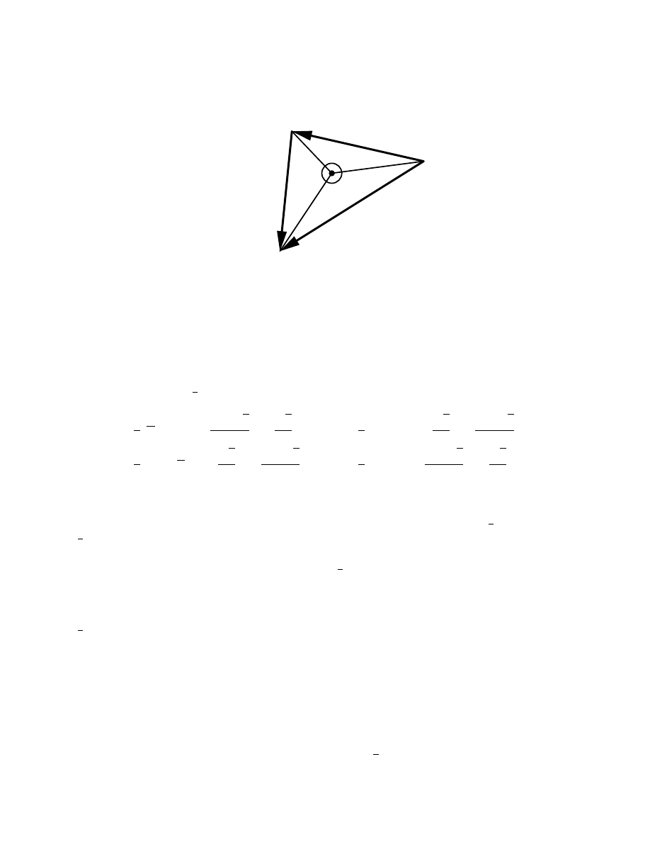
v + w + z
Figure 1.
Non–associativity.
b
C ⊂ L passing through ˆz and which projects back down to C. In particular, if C is a
closed curve, then b
C is also closed if and only if the winding number of C with respect to
−1 is zero.
We shall endow L with the structure of a connected, regular local Lie group which does
not satisfy the global associativity property, and hence cannot be contained in any global
Lie group. The group multiplication law on L will, locally, agree with vector addition
on
R
2
. The identity element will be the element ˆ
e = (1, 0) lying in the zero
th
sheet
of L which projects to e = 0, the identity element of the abelian Lie group G. The
multiplication µ(ˆ
z, ˆ
w) between two elements ˆ
z, ˆ
w ∈ L will be defined provided one or the
other is sufficiently close to the identity. When defined, the product ˆ
v = µ(ˆ
z, ˆ
w) will have
projection v = z + w in M . Moreover, the product µ(ˆ
z, ˆ
w) itself is defined either by lifting
the line segment connecting z to z + w to form a curve connecting ˆ
z to µ(ˆ
z, ˆ
w) in L, or,
alternatively, by lifting the segment connecting w to z + w to connect ˆ
w to µ(ˆ
z, ˆ
w). Note
that the lifted line segment will be unambiguously defined as long as the line segment in
question does not pass through the forbidden point −1.
Our goal is to suitably prescribe the domain of definition of the product µ so that all
three local group axioms are valid, (and the group is even locally commutative!), but then
prove that the group fails to satisfy the globally associativity property. The key technical
complication is to appropriately restrict the domain of definition of µ so that the ordinary
associativity law (1) holds. Note that if we allow too large a domain of definition, then
the resulting local group will only be locally associative. Indeed, let ˆ
v, ˆ
w, ˆ
z ∈ L be group
elements whose projections v, w, z, have the property that the triangle with vertices z,
w + z, v + w + z, contains the singular point −1 in its interior (and hence the triangle
has nonzero winding number); see Figure 1. Then the product µ(ˆ
v, µ( ˆ
w, ˆ
z)) cannot equal
µ(µ(ˆ
v, ˆ
w), ˆ
z) since the final points would have to lie on different sheets of the covering space
L. In this way, we see that associativity of an n-fold product is related to the winding
number of a certain polygonal path with respect to the distinguished point −1.
10
r
θ
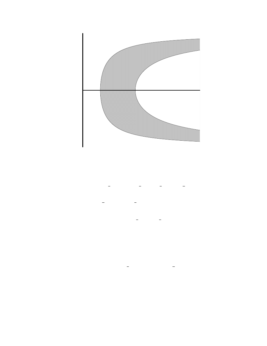
Figure 2.
The domain L
0
⊂ L.
The domain of definition of the product on L will now be fixed as follows. Let
L
0
=
©
(r, θ)
¯
¯
1
2
sec θ < r <
3
2
sec θ, −
1
2
π < θ <
1
2
π
ª
(4)
denote that part of the zero
th
sheet of L (i.e., the sheet containing the identity ˆ
e) which
lies above the strip M
0
= {−
1
2
< Re z <
1
2
}; see Figure 2. Note that the projection
π: L
0
→ M
0
is one-to-one when restricted to L
0
. Further let
L
1
=
©
(r, θ)
¯
¯ −
1
2
π < θ <
1
2
π
ª
(5)
denote that part of the zero
th
sheet of L which projects diffeomorphically onto the half
plane M
1
= {Re z > −1}. A trivial, but important observation is that if z, w ∈ M
0
, then
z + w ∈ M
1
.
Given z, w ∈ M, we let −π < α(z, w) ≤ π denote the angle from z to w with respect
to the singular point −1; see Figure 3. Given z ∈ M, define
H
z
=
©
ˆ
w ∈ L
0
¯
¯ −
1
2
π < α(z, z + w) <
1
2
π
ª
.
(6)
The domain of definition of the group operation is then taken to be
U = { (ˆz, ˆ
w) ∈ L × L | ˆz ∈ H
w
or
ˆ
w ∈ H
z
} .
(7)
In other words, the product µ(ˆ
z, ˆ
w) is defined provided either ˆ
w ∈ H
z
or ˆ
z ∈ H
w
. In the
former case, ˆ
w ∈ H
z
, and the product is defined by lifting the line segment connecting z to
z + w to form a connected curve from ˆ
z to µ(ˆ
z, ˆ
w) in L; in the latter case, ˆ
z ∈ H
w
, we lift
11
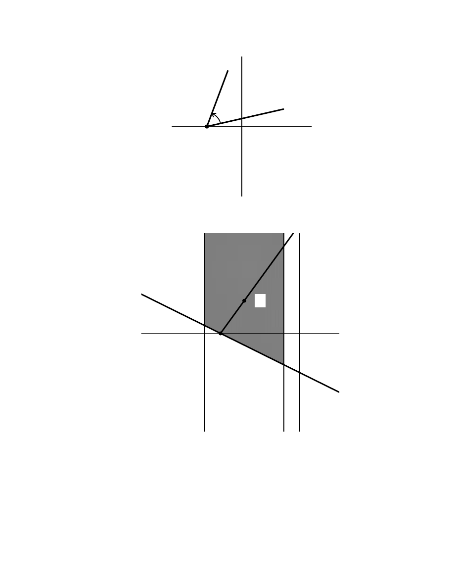
− 1
z
w
α
Figure 3.
The angle α = α(z, w).
− 1
z
Figure 4.
The domain of definition of the product.
the segment connecting w to z + w to connect ˆ
w to µ(ˆ
z, ˆ
w). Note that the restriction on
the domain implies that the line segment in question does not pass through the forbidden
point −1, and hence the lifted line segment is unambiguously defined. Given a point ˆz with
projection z, the shaded region in Figure 4 represents the projection of the set of possible
products µ(ˆ
z, ˆ
w) for all ˆ
w ∈ H
z
; the domain H
z
is obtained by translating the figure so as
to place z at the origin. Further, we define the domain of definition of the inversion map
12
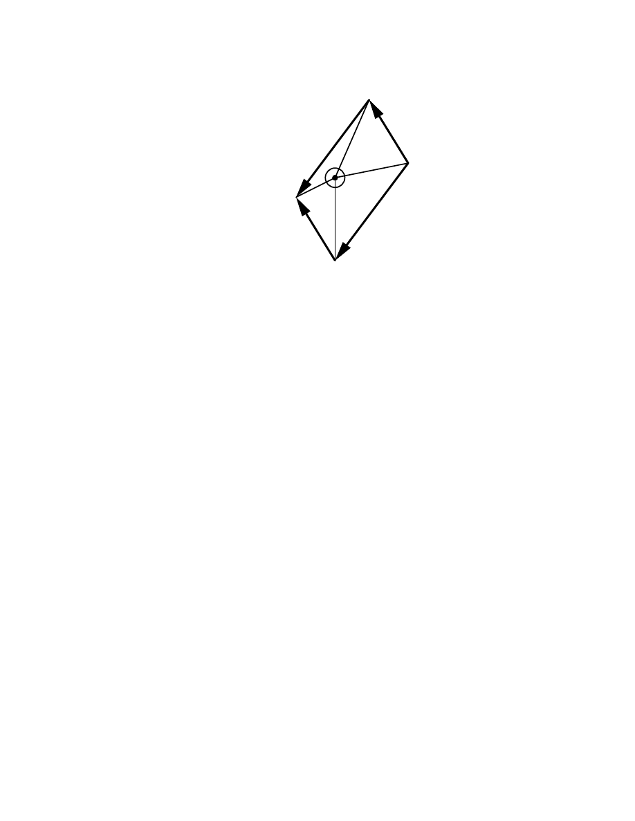
− 1
w
w + z
v + w + z
v + w
Figure 5.
Fundamental parallelogram.
ι to be V = L
0
, as given in (4). Given ˆ
z ∈ L
0
, the inverse ι(ˆ
z) is the unique element in L
0
projecting to −z.
Theorem 15.
Under the above constructions, the product
µ: U → L and inversion
ι: V → L endow L with the structure of a regular, connected, associative, local Lie group
which is not globally associative.
Proof
: The identity and inverse requirements are immediate. Local associativity of L
is also not difficult. To prove that L is associative (to order 3) we need to show that
µ(ˆ
v, µ( ˆ
w, ˆ
z)) = µ(µ(ˆ
v, ˆ
w), ˆ
z),
(8)
whenever both sides of the equation are defined. The left-hand side of (8) is defined
provided either a) ˆ
z ∈ H
w
or b) ˆ
w ∈ H
z
, and either a) ˆ
v ∈ H
w
+z
or b) µ( ˆ
w, ˆ
z) ∈ H
v
,
leading to four different possibilities. Similarly, there are four different ways that the right
hand side could be defined: a) ˆ
v ∈ H
w
or b) ˆ
w ∈ H
v
, and a) ˆ
z ∈ H
v
+w
or b) µ(ˆ
v, ˆ
w) ∈ H
z
.
Therefore, there is a grand total of sixteen different ways in which (8) could make sense!
We label the different possibilities by four letters, each either a or b, indicating which
one of the preceding different possibilities; for example, Case abba would require ˆ
z ∈ H
w
,
µ( ˆ
w, ˆ
z) ∈ H
v
, ˆ
w ∈ H
v
, and ˆ
z ∈ H
v
+w
. The sixteen cases subdivide into four classes, each
of which is handled by a slightly different proof.
The first class consists solely of Case aaaa, which means ˆ
z ∈ H
w
, ˆ
v ∈ H
w
+z
, ˆ
v ∈ H
w
,
ˆ
z ∈ H
v
+w
. Consider the fundamental parallelogram, defined as the parallelogram contained
in M with vertices w, v + w, w + z and v + w + z — see Figure 5. Clearly, the associative
law (8) holds in this case if and only if the point −1 does not lie in the interior of this
fundamental parallelogram. In Case aaaa, the four angles
α(w, w + z),
α(w + z, v + w + z),
α(w, v + w),
α(v + w, v + w + z),
13
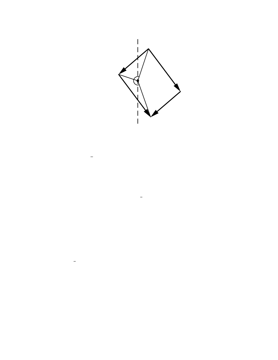
− 1
w
w + z
v + w + z
v + w
Figure 6.
Case abaa.
are all strictly less than
1
2
π, which, as illustrated in Figure 5 immediately implies that the
fundamental parallelogram cannot contain −1.
The second class is exemplified by Case abaa, which requires ˆ
z ∈ H
w
, µ( ˆ
w, ˆ
z) ∈ H
v
,
ˆ
v ∈ H
w
, ˆ
z ∈ H
v
+w
. In this case, v, z, w + z ∈ M
0
, and hence w = (w + z) − z and v + w + z
lie in M
1
. This means that the only vertex of the fundamental parallelogram which can lie
to the left of the line {Re z = −1} is v + w. On the other hand, the two angles α(w, v + w)
and α(v + w, v + w + z) must be less than
1
2
π, which is impossible unless v + w ∈ M
1
also — see Figure 6. Thus −1 is not contained in the fundamental parallelogram, and
associativity holds here also. Similar arguments apply to Cases aaab, aaba, aabb, baaa,
and baba.
The third class is indicated by Case baab, which requires ˆ
w ∈ H
z
, ˆ
v ∈ H
w
+z
, ˆ
v ∈ H
w
,
µ(ˆ
v, ˆ
w) ∈ H
z
. In this case, consider the fundamental triangle with vertices at z, w + z and
v + w + z, as illustrated in Figure 7. The three angles
α(z, v + w + z),
α(z, w + z),
α(w + z, v + w + z),
are all less than
1
2
π, hence the triangle cannot contain −1 in its interior. Therefore, the
corresponding three points lie on the same sheet of L, and associativity holds. Similar
arguments apply to Cases abba, babb, and bbba.
The final, and easiest class is exemplified by Case abab. Here ˆ
z ∈ H
w
, µ( ˆ
w, ˆ
z) ∈ H
v
,
ˆ
v ∈ H
w
, µ(ˆ
v, ˆ
w) ∈ H
z
. Thus v, z, v + w, w + z ∈ M
0
, and hence w, v + w + z ∈ M
1
.
Thus every vertex of the fundamental parallelogram lies to the right of −1, so −1 is not
contained in its interior, and hence associativity holds. The same argument applies to
Cases abbb, bbaa, bbab, and bbbb. We have now analyzed every one of the sixteen different
possibilities, and hence associativity of our local Lie group is proved.
To prove global non-associativity, it suffices to produce one counter-example to the
14
− 1
z
w + z
v + w + z
Figure 7.
Fundamental triangle.
next simplest associative identity:
µ(ˆ
u, µ(ˆ
v, µ( ˆ
w, ˆ
z))) = µ(µ(µ(ˆ
u, ˆ
v), ˆ
w), ˆ
z)).
(9)
This will demonstrate that L is not associative of order 4, and, hence, not globally asso-
ciative. Let ω = exp
1
4
πi be the primitive eighth root of unity. Let
u =
2
3
(ω − 1) = −
2 −
√
2
3
− i
√
2
3
,
v =
2
3
(−i − ω) = −
√
2
3
− i
2 −
√
2
3
,
w =
2
3
(i − ω) = −
√
2
3
+ i
2 −
√
2
3
,
z =
2
3
(ω − 1) =
2 −
√
2
3
+ i
√
2
3
.
(10)
Finally, let ˆ
u, ˆ
v, ˆ
w, ˆ
z be the corresponding points in L
0
which project to u, v, w, z. Note
that, as illustrated in Figure 8, the points 0, u, u + v, u + v + w, u + v + w + z, v + w + z,
w + z, and z form the vertices of a regular octagon centered at the point −
2
3
having radius
2
3
. In particular, this implies that the singular point −1 lies inside the octagon, and hence
any lift of the octagon does not form a closed curve in the covering space L. Therefore,
if we start at 0, and go to u + v + w + z = −
4
3
along the two different polygonal paths,
we will end up at different points back up on the covering space L, which implies that the
associativity condition (9) does not hold! We leave it to the reader to check that both
four-fold products are well defined — in particular that the relevant angles are all less than
1
2
π. This produces the required example.
The only remaining point is to show that L satisfies the connectivity conditions in
Definition 13, but this is fairly straightforward. First, L itself is clearly pathwise connected,
as is V = L
0
. The domain (7) is also pathwise connected. Indeed, consider a point
(ˆ
z, ˆ
w) ∈ U such that ˆ
w ∈ H
z
. We can connect (ˆ
z, ˆ
w) to (ˆ
z, 0) by a curve {ˆz} × S, where
S ⊂ H
z
is the lift of the straight line segment that connects w to 0. Further, since L is
pathwise connected, we can then connect (ˆ
z, 0) to (0, 0) via a curve C ×{0} ⊂ L×{0}. The
alternative case ˆ
z ∈ H
w
is handled analogously, thus proving that U is pathwise connected.
Finally, note that the open set U = { ˆz ∈ L
0
| |z| <
3
4
} generates L. Indeed, repeatedly
15

v
w
z
w
v
u
u
z
Figure 8.
Non–associative octagon.
multiplying the primitive eighth root elements ˆ
u, ˆ
v, ˆ
w, ˆ
z ∈ U constructed above, cf. (10),
allows us to circle the singular point −1 as many times as we like in order to reach any
desired sheet of L. Once on a given sheet, it is straightforward to continue to multiply by
appropriate elements of U to generate any group element lying in that sheet. Moreover,
any open subneighborhood e ∈ e
U ⊂ U ⊂ L will clearly generate U, thereby verifying the
last connectivity requirement. This at last completes the proof of the theorem.
Q.E.D.
Finally, we remark that one can suitably shrink the domain of definition of the product
on L, enabling one to construct a local Lie group that is associative to order n, but which
is not globally associative. The precise definition of the n
th
order domain, though, is rather
tricky, owing to the many possible n-fold products that may be defined!
The examples modeled on the covering space of M =
R
2
\ {−1} are not globally inver-
sional, since the inverse was only defined for group elements ˆ
z ∈ V = L
0
. A modification
of this basic construction can, though, be used to produce a globally inversional, but not
globally associative local Lie group. We briefly indicate how this can be accomplished. The
key is that the group domain needs to be symmetric with respect to the origin, while still
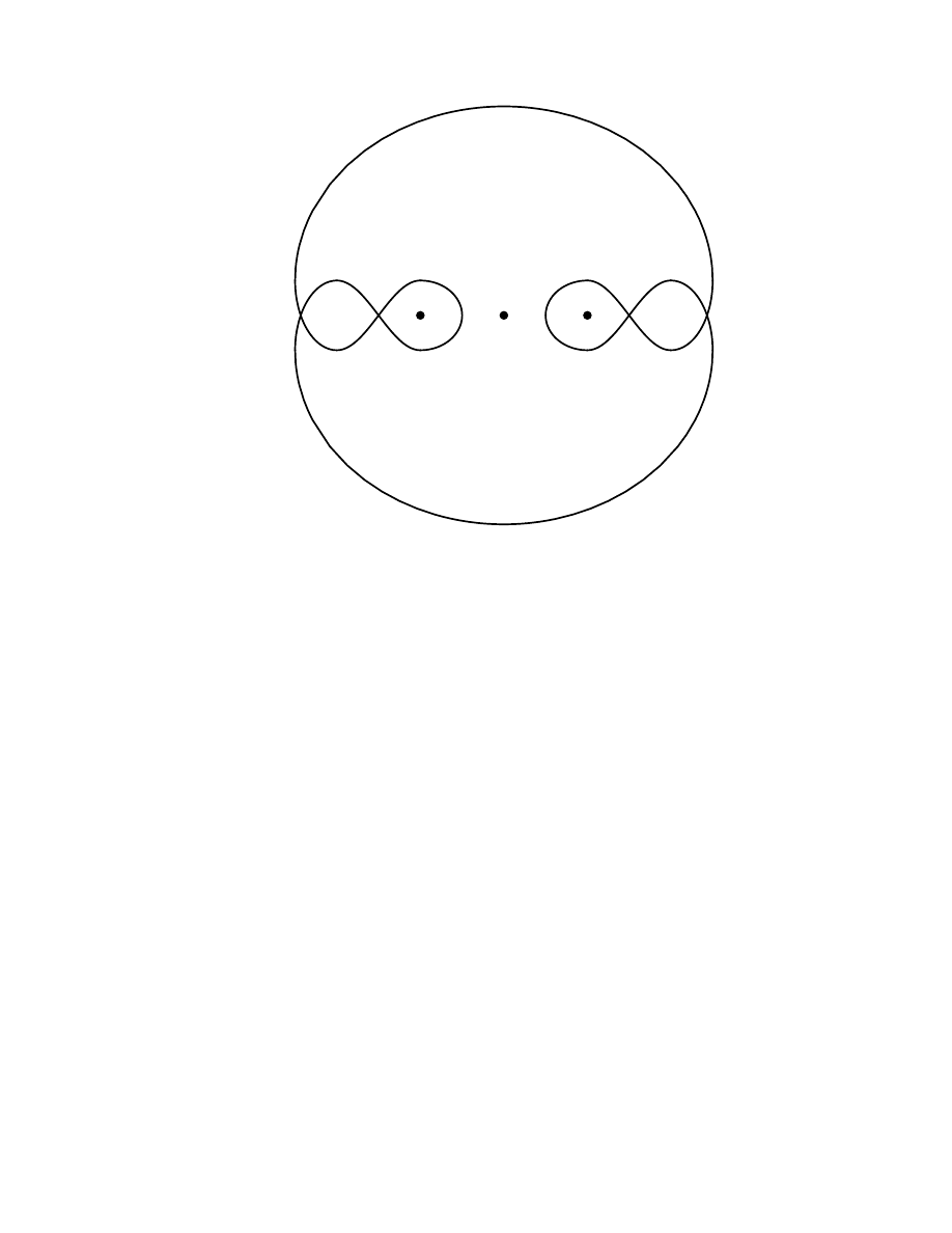
maintaining non-associativity. Consider the twice punctured plane f
M =
R
2
\ {+1, −1},
and let π: f
M ∗ → f
M denote the simply connected covering space of f
M ; we can identify f
M ∗
with the Riemann surface corresponding to the complex function log(z
2
− 1). Fix a point
e ∈ π
−1
{0} as the identity. Let e
L ⊂ f
M ∗ be a domain which contains e, which is four-
fold symmetric under the analytic continuation of the coordinate axis reflections z 7→ ¯z,
z 7→ −¯z, and whose projection overlaps itself on the outer real axes { (x, 0) | |x| > 1 } just
once. See Figure 9 for a sketch of the projection of such a domain. Clearly, by symmetry,
we can arrange e
L to be globally inversional by analytic continuation of the inversion map
z 7→ −z lifted to f
M ∗. Thus, the inverse of an element ˆ
z that lies in the upper sheet of e
L
that is to the right of +1 will end up in the lower sheet of e
L that is to the left of −1. It is
16
− 1
0
1
Figure 9.
Globally inversional non–associative local Lie group.
also clear, that by suitably restricting the domain of definition of the product, which will
be the lift of the usual vector addition as in our previous example, one can endow e
L with
the structure of a globally inversional, abelian, local Lie group. Nevertheless, due to the
overlap of the projection of e
L back down to f
M , the resulting local Lie group is clearly not
globally associative. The precise definition of the domain of definition of the product on
e
L so as to make it associative to order, say, 3, but not to order 4, is left as a (challenging)
exercise for the reader.
4.
A General Characterization of Local Lie Groups.
The basic construction in the previous section can be readily generalized to apply to
covering spaces of open subsets of arbitrary Lie groups. The main technical complication
is the determination of a suitably small domain of definition of the multiplication map so
as to maintain local associativity. The existence of such a domain is straightforward —
one merely ensures that the corresponding “polygonal paths” do not encircle any of the
components of the complement of the open subset. However, an explicit construction in
particular examples can get complicated.
We now investigate in what sense these are the most general examples. The main
result states that this is the case “up to covering”. Here, though, our definition of covering
is more general than usual.
Definition 16.
A local diffeomorphism Φ: M → N between two m-dimensional
manifolds M and N which is onto is called a generalized covering map.
17

Thus, according to the Inverse Function Theorem, a map Φ: M → N is a generalized
covering map if and only if Φ(M ) = N and dΦ: T M |
x
→ T N|
Φ(x)
is an invertible linear
map for each x ∈ M. Our use of the term “covering map” is more inclusive than the usual
terminology, since M does not necessarily cover N uniformly; indeed the inverse image
Φ
−1
(y) of a point y ∈ N is a discrete subset of M, but its cardinality may vary from
point to point. For instance, according to our definition, the restriction of any generalized
covering map to any open subset f
M ⊂ M such that Φ( f
M ) = N remains a generalized
covering map. For example, the map F (t) = (cos t, sin t) provides an ordinary covering
map from the real line M =
R to the circle N = S
1
, which remains a generalized covering
map when restricted to any open interval of length at least 2π. By abuse of terminology,
we will say M covers N if there is a generalized covering map from M to N .
If L and L are local Lie groups, we will say that L is a covering group of L if there
is a generalized covering map Φ: L
→ L which is a local group homomorphism. A simple
example is provided in Section 3, where the non-associative local Lie group L is realized
as a covering group of the globally associative local Lie group M ⊂ R
2
. A more exotic
example of a local Lie group is found by starting with the local Lie group L described in
Section 3, and choosing a point ˆ
e 6= ˆz
0
∈ L. Then the simply connected covering space
L → L \ {ˆz
0
} is also a (non-uniform) local covering group of M.
We next recalling some standard facts concerning frames and coframes on manifolds
and (local) Lie groups.
Definition 17.
Let M be a smooth m-dimensional manifold. A frame on M is an
ordered set of vector fields V = {v
1
, . . . , v
m
} having the property that they form a basis
for the tangent space T M |
x
at each point x ∈ M. Dually, a coframe on M is an ordered
set of one-forms θ = {θ
1
, . . . , θ
m
} which form a basis for the cotangent space T ∗M|
x
at
each point x ∈ M.
A manifold admits a (global) frame if and only if its tangent bundle is topologically
trivial: T M ' M × R
m
. The structure equations associated with a frame are obtained by
expressing the Lie brackets in terms of the frame vector fields themselves:
[v
i
, v
j
] =
m
X
k
=1
C
k
ij
v
k
,
i, j = 1, . . . , m.
(11)
The coefficient functions C
k
ij
are called the structure functions of the given frame. The
frame is said to have rank 0 if the structure coefficients C
k
ij
are all constant. In this case,
the C
k
ij
form the structure constants of the Lie algebra g spanned by the frame vector
fields. We will show that we can endow M itself with the structure of a local Lie group
such that the frame vector fields form a basis for the Lie algebra g of right-invariant
†
vector
fields thereon.
Theorem 18.
If
L is a regular, locally associative, local Lie group, then it admits a
right invariant frame of rank 0. Conversely, if
M is a manifold that admits a rank 0 frame,
†
One can equally well use left-invariant vector fields if one prefers.
18

then
M can be endowed with the structure of a regular, locally associative local Lie group
having the given frame as right-invariant Lie algebra elements.
Proof
: Let L be the m-dimensional local Lie group in question. We first construct
the Lie algebra g consisting of all right-invariant vector fields on L by standard methods,
cf. [28]. In other words, given a tangent vector v|
e
∈ T L|
e
to L at the identity, we define its
right-invariant counterpart to be the vector field with value v|
x
= dρ
x
(v|
e
) at any x ∈ L,
where ρ
x
denotes the standard right multiplication map, cf. (3). Associativity implies the
right-invariance of v, so dρ
y
(v|
x
) = v|
µ
(x,y)
for any (x, y) ∈ U. The regularity hypothesis
implies that g defines a global frame on L, i.e., we can choose a basis
b
v
1
, . . . ,
b
v
m
which span
the tangent space T L|
x
at each point x ∈ L, satisfy the standard Lie algebra commutation
relations (11) for structure constants C
k
ij
relative to the chosen basis.
Remark
: If the group does not satisfy our regularity assumption, then the construction
of the right-invariant frame leads to degeneracies at the “infinite elements”. For instance,
in the irregular Example 7, the right-invariant vector field
b
v
= (x − 1)
2
∂
x
vanishes at the
infinite element x = 1.
To prove the converse, let G denote the global Lie group whose Lie algebra has the
given structure constants determined by the structure equations (11) of the rank 0 frame.
According to the basic theorem on transformation groups, [28; Theorem 88], [23; Theorem
1.57], the vector fields v
i
form the infinitesimal generators for a local action of G on M .
In particular, we can choose any point e ∈ M to serve as the identity element for the
local group structure on M , and the map g 7→ g · e serves to define a group isomorphism
between a sufficiently small neighborhood of e ∈ M with a neighborhood of the identity
in G. In this way, we can identify the transformation x 7→ g · x by a group element g ∈ G
sufficiently close to the identity with the product g · x = µ(y, x) by the corresponding
element y = g · e ∈ M. Thus, by suitably restricting the domain of definition of the
transformation group action, we endow M with the structure of a local Lie group. The
construction of the associated inverse map and verification of the local group axioms is
straightforward.
Q.E.D.
Any manifold admitting a global frame V = {v
1
, . . . , v
m
} also admits a global coframe
provided by the dual one-forms θ = {θ
1
, . . . , θ
m
}, and conversely. These are constructed
so that
θ
i
; v
j
®
= δ
i
j
at each x ∈ M, where δ
i
j
is the usual Kronecker symbol. The dual
structure equations for the coframe are
dθ
k
= −
X
1≤i<j≤m
C
k
ij
θ
i
∧ θ
j
,
(12)
and have the same (up to sign) structure functions C
k
ij
. In particular, the dual coframe to
a right-invariant frame on a local Lie group is known as the Maurer–Cartan coframe, and
(12) are the fundamental Maurer–Cartan structure equations, with the C
k
ij
the structure
constants for the Lie algebra. Note that Theorem 18 immediately implies that any manifold
admitting a rank 0 coframe can be given the structure of a local Lie group.
Theorem 19.
If
L is a regular, locally associative local Lie group, then it admits
a right invariant Maurer–Cartan coframe satisfying the rank 0 structure equations
(12).
19

Conversely, if
M is a manifold with a coframe of rank 0, then M can be endowed with
the structure of a regular, locally associative local Lie group having the given coframe as
Maurer–Cartan coframe.
Remark
: The preceding considerations imply that any smooth, connected local Lie
group comes equipped with a Cartan connection θ: T L → g with vanishing curvature
Ω = dθ + [θ, θ] = 0. See [20], [30], for the theory of “almost Lie groups” in which
one relaxes this condition by allowing manifolds with a Cartan connection having small
curvature. Under certain conditions, such manifolds are necessarily local Lie groups.
Finally, we state the basic infinitesimal characterization of local Lie group homeomor-
phisms.
Theorem 20.
Suppose
L and M are connected m-dimensional local Lie groups, and
let θ and η denote their respective right-invariant Maurer–Cartan coframes. If a map
Φ: L → M satisfies Φ∗(η) = θ and Φ(e) = ˜e, then Φ defines a local group homeomorphism
from
L onto its image, which forms an open local subgroup of M .
Proof
: The pull-back conditions imply that the corresponding dual right-invariant
vector fields are mapped to each other by the push forward map: dΦ(v
i
) = w
i
, i =
1, . . . , m. Therefore Φ is equivariant under the associated flows or one-parameter subgroup
actions: Φ(exp(tv)y) = exp(tw)Φ(y), where v = c
1
v
1
+ · · · + c
m
v
m
∈ g and t is sufficiently
small. Therefore, the homeomorphism property
Φ(µ(x, y)) = e
µ(Φ(x), Φ(y))
(13)
holds provided x = exp(tv) for v ∈ g and t sufficiently small. Now, the exponential map
maps an open neighborhood of 0 ∈ g onto a neighborhood of e ∈ L, and hence (13) holds
whenever x ∈ L is sufficiently close to the identity. Since L is connected, we can use
continuity of Φ to assert that (13) holds for all (x, y) ∈ U. The corresponding assertion
for the inversion is proved similarly, completing the proof.
Q.E.D.
Our main result will completely characterize local Lie groups up to (generalized)
covering. The proof relies on the Cartan equivalence method, [7], [10], applied to coframes
of rank zero, which in turns rests on an application of Frobenius’ Theorem to construct
the covering map via Cartan’s technique of the graph. See [24] for additional details.
Theorem 21.
Let
L be a connected local Lie group. Then there exists a local
covering group
L → L which is also a local covering group L → M of an open subset
M ⊂ G of a global Lie group G.
Proof
: Let L be a local group and let θ = {θ
1
, . . . , θ
m
} be its Maurer–Cartan coframe.
The structure equations (12) serve to define the structure constants of an m-dimensional
Lie algebra g. Let G denote the connected, simply connected, m-dimensional global Lie
group having the same Lie algebra g. Let α = {α
1
, . . . , α
m
} be the corresponding Maurer–
Cartan coframe of globally right-invariant one-forms on G with respect to the same basis
of g. The Maurer–Cartan structure equations of α are the same as those of θ, cf. (12).
Thus, according to the Cartan equivalence method, [7], [10], [24], if x ∈ L and g ∈ G
20

are any two elements, then there is a unique local equivalence map Φ: L → G, defined in
a neighborhood of x, such that Φ(x) = g and Φ pulls-back the Maurer–Cartan coframe on
G to that on L, so Φ∗(α) = θ. In particular, if we take x = e to be the identity element of
L, and g = e the identity element of G, then Theorem 20 implies that Φ is a local group
homeomorphism from a neighborhood of the identity in L to a neighborhood of e ∈ G.
The map Φ serves to globalize a neighborhood of the identity in L, thereby reproducing
Cartan’s global version, [6], of Lie’s Third Fundamental Theorem. (Of course, this is
cheating, since we have assumed the existence of the appropriate global Lie group G in
advance!)
To see how Φ can itself be globalized, we need to understand its construction in more
detail. The proof of the local equivalence result is based on Cartan’s technique of the
graph. One determines the local equivalence map Φ: L → G by constructing its graph
Γ
Φ
= {(x, Φ(x)}, which is a r = dim G dimensional submanifold of the Cartesian product
space L × G. The graph is realized as an integral submanifold of a suitable differential
system I, namely the one generated by the differences ϑ
i
= π∗
G
α
i
− π∗
L
θ
i
, i = 1, . . . , m,
of the pull-backs of the two coframes under the standard projections π
L
: L × G → L
and π
G
: L × G → G. The fact that the two coframes have identical constant structure
coefficients implies that this differential system is in involution, and hence Frobenius’
Theorem, cf. [24], [36], guarantees the existence of a unique maximal integral submanifold
N , of dimension m, passing through any point (x, g) ∈ L × G. The integral submanifold
N coincides, locally, with the graph of the required equivalence map Φ. The fact that N
satisfies the required transversality conditions at (x, g) is immediate, and so the Implicit
Function Theorem guarantees that it defines a local diffeomorphism.
In order to complete the proof, we need to show that the full maximal integral subman-
ifold covers all of L. Let N ⊂ L×G denote the maximal integral submanifold corresponding
to the differential system described above passing through the point (e, e) ∈ L × G. We
know that, locally, N is the graph of an equivalence map. Indeed, the restrictions of the
two projections π
L
: N → L, π
G
: N → G, determine local diffeomorphisms. Moreover,
equivalence implies that the given coframe θ on L and the Maurer–Cartan coframe α on
G both pull back to the same rank 0 coframe, ξ = π∗
L
θ
= π∗
G
α
on N . According to
Theorem 19, the existence of a rank zero coframe on N allows us to identify it as a local
Lie group with the point (e, e) serving as the identity element. Moreover, Theorem 20
implies that the two (generalized) covering maps will then be local group homomorphisms.
In fact, since the one-forms in ξ form a subset of the Maurer–Cartan coframe on the local
product group L × G, consisting of the one-forms π∗
L
θ
, π∗
G
α
, the local group structure on
N coincides with the restriction of the Cartesian product local group structure on L × G,
and so we can identify N as an m-dimensional local Lie subgroup of L × G.
I claim that the restricted projection π
L
: N → L is, in fact, a generalized covering
map, which requires us to prove that π
L
(N ) = L. Assuming this, the theorem follows
directly, since N will then be the required covering group of L, and also cover an open
subset of G under π
G
, thereby fulfilling the conditions of Definition 16. To prove the claim,
note that if N is any integral submanifold of the differential system generated by ϑ, then,
because of the right-invariance of the Maurer–Cartan forms, any right translate ρ
h
[N ] =
{ (x, g · h) | (x, g) ∈ N } by a group element h ∈ G is also an integral submanifold. Suppose
21

L
G
N
N
0
x
0
h
g
^
x
^
g
~
Figure 10.
Integral submanifolds.
π
L
(N ) 6= L, and let x
0
∈ L \ π
L
(N ) be a point in the closure of π
L
(N ). According to
Frobenius’ Theorem, we can find a local equivalence Φ
0
: U → G, where U is a neighborhood
of x
0
in L, mapping x
0
to the identity element e = Φ
0
(x
0
); see Figure 10. Let N
0
denote
the graph of Φ
0
, so that N
0
is also an integral submanifold of our differential system
passing through (x
0
, e). Choose any point ˆ
x ∈ U ∩ π
L
(N ), so ˆ
x = π
L
(ˆ
x, ˆ
g) for some point
(ˆ
x, ˆ
g) ∈ N in the original integral submanifold. Let ˜g = Φ
0
(ˆ
x), and define h = ˜
g
−1
· ˆg.
Then, by the previous remark, R
h
[N
0
] is an integral submanifold of the differential system;
moreover, the point (ˆ
x, ˆ
g) = (ˆ
x, ˜
g·h) is contained both in ρ
h
[N
0
] and in our original integral
submanifold N . Therefore, by uniqueness and maximality of N , the integral submanifold
ρ
h
[N
0
] must be an open submanifold of N . But the point (x
0
, h) = ρ
h
(x
0
, e) lies in ρ
h
[N
0
],
and hence in N . This contradicts our original assumption that x
0
was not in the projection
π
L
(N ), and so proves the claim.
Q.E.D.
Example 22.
Consider the coframe
θ
1
= cos ϕ dr − r sin ϕ dϕ,
θ
2
= sin ϕ dr + r cos ϕ dϕ,
(14)
defined on the half plane L = { (r, ϕ) | r > 0 }. Clearly, in terms of polar coordinates,
this coframe is locally diffeomorphic to the Maurer–Cartan coframe α
1
= dx, α
2
= dy for
the two-dimensional abelian Lie group
R
2
. Indeed, L can be identified with the simply
connected covering space for the punctured plane M =
R
2
\{(−1, 0)}, and so is isomorphic
to our earlier example of a non-associative local Lie group. Consequently, this coframe
is the Maurer–Cartan coframe for the local Lie group L and is therefore not globally
equivalent to the Maurer–Cartan coframe on any open subset of the Lie group
R
2
.
22

This example includes yet one additional interesting pathology. The dual frame vector
fields to (14) are
v
1
= cos ϕ
∂
∂r
−
sin ϕ
r
∂
∂ϕ
,
v
2
= sin ϕ
∂
∂r
+
cos ϕ
r
∂
∂ϕ
.
(15)
They are mapped to the coordinate vector fields ∂
x
, ∂
y
under the polar coordinate map,
and hence commute:
[v
1
, v
2
] = 0.
(16)
Nevertheless, their flows do not commute! The reader can explicitly verify that, for any
r
0
> 0, if we set s = t =
√
2 r
0
, then
exp(sv
1
) exp(tv
2
)
¡
r
0
,
5
4
π
¢
= exp(sv
1
)
¡
r
0
,
3
4
π
¢
=
¡
r
0
,
1
4
π
¢
,
whereas
exp(tv
2
) exp(sv
1
)
¡
r
0
,
5
4
π
¢
= exp(tv
2
)
¡
r
0
,
7
4
π
¢
=
¡
r
0
,
9
4
π
¢
.
(This is easy to do by reverting to rectangular coordinates.) Thus we have an explicit,
elementary counterexample to the commutativity theorem in [23; Theorem 1.34], which
states that two vector fields on a manifold M satisfy (16) if and only if their flows satisfy
exp(sv
1
) exp(tv
2
)x
0
= exp(tv
2
) exp(sv
1
)x
0
,
(17)
for all x
0
∈ M and all (s, t) ∈ V where V denotes the subset of the s, t plane where both
sides of (17) are defined! This theorem, that commuting vector fields induce commuting
flows, is true locally. A correct version should state that (17) holds for all (s, t) lying in the
connected component of V containing the origin. In the above example, for x
0
=
¡
r
0
,
5
4
π
¢
,
the left hand side of (17) is defined for all (s, t) ∈ V
1
=
R
2
\ {s =
1
√
2
r
0
, t ≥
1
√
2
r
0
}. The
right hand side of (17) is defined for all (s, t) ∈ V
2
=
R
2
\ {t =
1
√
2
r
0
, s ≥
1
√
2
r
0
}. The
set V = V
1
∩ V
2
on which both sides of (17) are defined, then, consists of two connected
components, V = W
0
∪ W
1
. If (s, t) ∈ W
0
= {s <
1
√
2
r
0
ort <
1
√
2
r
0
}, which is the
component containing the origin, the commutativity equation (17) holds. On the other
hand, when (s, t) ∈ W
1
= {s >
1
√
2
r
0
andt >
1
√
2
r
0
}, commutativity equation (17) does not
hold.
Remark
: Using a version of the Hopf–Rinow Theorem, Gardner, [10; p. 72], shows
that a rank zero coframe θ = {θ
1
, . . . , θ
m
} on a simply connected manifold M which is
metrically complete with respect to the Riemannian metric
P
i
(θ
i
)
2
induced by the coframe
is globally equivalent to a Maurer–Cartan coframe on a global Lie group. Thus, metric
completeness is, in some subtle way, related to associativity.
Remark
: The covering map π
L
: N → L identifies (in a neighborhood of each point)
the local group structure on N with some restriction of the local group structure on L.
An open question is whether this too can be globalized: Can we construct a covering local
group π: N → L such that every well-defined product µ(x, y), and inverse ι(x) has its
counterpart in N . In other words, if e
U and e
V denote the local group domains for L, can
we ensure that (π × π) e
U → U and π(e
V) → V are also covering maps? This appears
to be more difficult, in light of the global incompatibility of locally homeomorphic group
structures on a given local Lie group.
23

5.
Globalization.
Finally, we prove a version of Mal’cev’s Theorem, [19], that the condition of global
associativity is both necessary and sufficient for a local Lie group to be contained in a
global Lie group. Here we adapt Mal’cev’s method of proof, and generalize his result to
connected (and hence inversional) local Lie groups. Mal’cev argument extremely brief, and
is not entirely convincing at first sight, so we need to fill in some of the missing details.
Moreover, Mal’cev assumes that the group is globally inversional, so we need to include
additional arguments to cover mere inversionality. The fundamental result relies on the
basic Definition 6 of a globalizable local Lie group.
Theorem 23.
A connected local Lie group
L is globalizable if and only if it is
globally associative.
Proof
: The necessity of global associativity is clear. To prove its sufficiency, we must
construct a global Lie group G containing the given connected local Lie group L. Let
W = W(L) =
∞
[
n
=1
L
×n
denote the set of words based on the set L, i.e., ordered n-tuples (x
1
, . . . , x
n
) ∈ L
×n
for
any n ≥ 1. We define an equivalence relation on W as follows: If x
k
, x
k
+1
are adjacent
elements in an n-tuple X = (x
1
, . . . , x
n
) ∈ M such that (x
k
, x
k
+1
) ∈ U ⊂ L × L, then
X will be equivalent to the (n − 1)-tuple Y = (x
1
, . . . , x
k
−1
, y, x
k
+2
, . . . , x
n
) ∈ L
×(n−1)
obtained by replacing them by the product y = µ(x
k
, x
k
+1
) ∈ L. Vice versa, if an element
x
k
= µ(y
1
, y
2
) in X is written as a product of local group elements, then X will be
equivalent to the (n + 1)-tuple Z = (x
1
, . . . , x
k
−1
, y
1
, y
2
, x
k
+1
, . . . , x
n
) ∈ L
×(n+1)
obtained
by replacing x
k
by y
1
, y
2
. The first type of equivalence relation will be called a contraction
and the second an expansion. Thus two words X, Y ∈ W are equivalent if and only if there
is a finite chain of basic equivalences — expansions and contractions — starting with X
and ending with Y . Finally, we define G = W/ ∼ to be the set of equivalence classes under
the full equivalence relation. The claim is that G can be endowed with the structure of a
global, connected Lie group such that the map σ: L → G that identifies each x ∈ L with
the corresponding 1-tuple σ(x) = x ∈ L
×1
⊂ W is an injective local group homomorphism.
An associative product on W is given by juxtaposition of words. This product clearly
respects the equivalence relation, and hence provides a globally defined, globally associative
product on G. The inverse of an m-tuple Y = (y
1
, . . . , y
m
) ∈ V
×m
⊂ W consisting of
invertible elements y
i
∈ V ⊂ L is given by inverting the individual group elements and
reversing the order, so Y
−1
= (y
−1
m
, . . . , y
−1
1
). Clearly Y · Y
−1
and Y
−1
· Y are both
equivalent to the identity element in G. More generally, thanks to the regularity of L and
Proposition 14, given any (x
1
, . . . , x
n
) ∈ W, we can write each x
i
= y
i
1
· y
i
2
· . . . · y
ik
i
as a
product of invertible elements y
iν
∈ V, whereby X is equivalent to the element
X = (x
1
, . . . , x
n
) ∼ Y = (y
11
, . . . , y
1k
1
, y
21
, . . . , y
2k
2
, . . . , y
n
1
, . . . y
nk
n
).
The inverse of X in G can then be identified with the inverse of Y .
24

The global associativity of L ensures that this construction is well-defined on G,
making G into a group. At this point in his proof of [19; Theorem 1], Mal’cev merely
says “. . . on peut d´emontrer . . . ” that the global associativity assumption implies that
the map σ: L → G is an injective local group homomorphism. A detailed argument can
be constructed as follows: The fact that σ is a local group homomorphism is immediate
from the definition of the product on G. The difficulty is in the equivalence procedure,
which could conceivably prevent the injectivity of σ. This would mean that we might be
able to find two different local group elements x 6= z which admit a chain of equivalences
consisting of expansions and contractions. We must show that this cannot happen due to
our global associativity hypothesis. Now, if the chain of equivalences starting at x and
ending at z consists of a sequence of n expansions, increasing the word length by 1 at
each step, followed by a sequence of n contractions ending at z, which we refer to as a
simple equivalence chain
, then global associativity is applicable and we may conclude that
x = z. The desired conclusion is less clear if the chain of equivalences is not simple, mixing
expansions and contractions. However, this will reduce to the simple case if we can show
that all the intermediate contractions can be replaced by equivalent expansions, so that
the given chain of equivalences can be replaced by one of simple form.
Consider a contraction that replaces an adjacent pair x
k
, x
k
+1
of elements in a word
X by their product y = µ(x
k
, x
k
+1
). If x
k
∈ V is an invertible element sufficiently
close to the identity, then x
k
+1
= µ(x
−1
k
, z), and hence the singleton y ∈ L can be
replaced by the equivalent triple (x
k
, x
−1
k
, y) ∈ L
×3
, which we can also view as an ex-
pansion
of the pair (x
k
, x
k
+1
). More generally, using the connectivity of L, we expand
x
k
into an equivalent sequence x
k
1
, . . . , x
kn
of invertible elements x
kj
∈ V such that
y = µ(x
k
1
, µ(x
k
1
, . . . , µ(x
kn
, x
k
+1
) . . .)) and x
k
+1
= µ(x
−1
kn
, µ(x
−1
k,n
−1
, . . . , µ(x
−1
k
1
, y) . . .)).
We then replace y by the equivalent word (x
k
1
, . . . , x
kn
, x
−1
kn
, . . . , x
−1
k
1
, y), which can also
be regarded as a sequence of successive expansions of the original pair (x
k
, x
k
+1
). Al-
ternatively, we can replace y by the word (y, x
k
1
, . . . , x
kn
, x
−1
kn
, . . . , x
−1
k
1
), since, by global
associativity,
(y, x
1
, . . . , x
n
, x
−1
n
, . . . , x
−1
1
) ∼ y ∼ (x
1
, . . . , x
n
, x
−1
n
, . . . , x
−1
1
, x),
for any y ∈ L, and x
1
, . . . , x
n
∈ V. Thus, we can always ensure that adjacent group ele-
ments in the original words can always be arranged to be adjacent in the new expanded
words, and thus we can continue to replace each contraction in the original sequence
of equivalences by an equivalent expansion. Proceeding in this manner, we finally ar-
rive at an ultimate word that is composed of a large number of subwords of the form
(y
1
, . . . , y
k
, y
−1
k
, . . . , y
−1
1
) juxtaposed with the final singleton z at some position. We can
now follow our sequence of expansions by a sequence of elementary contractions, each one
replacing a pair y
j
y
−1
j
by e and then canceling out the e. Thus we have produced the
desired simple chain of equivalences connecting x to z. This completes our demonstration
that the map σ is injective.
Finally we demonstrate that G is a manifold and hence forms a global Lie group. The
second countability axiom follows immediately from the fact that W itself is second count-
able. We introduce local coordinates on G as follows: Given an n-tuple (x
1
, . . . , x
n
) ∈
L
×n
, we define its k
th
coordinate neighborhood to consist of all n-tuples of the form
25

(x
1
, . . . , x
k
−1
, y, x
k
+1
, . . . x
n
), where y lies in a sufficiently small local coordinate neighbor-
hood of x
k
∈ L. The smoothness of the overlap maps relies on global associativity. For
instance, the overlap map between the k
th
and (k + 1)
st
coordinate neighborhoods deter-
mined by a fixed n-tuple arises by assuming that y is sufficiently close to x
k
, which, by
regularity, implies that we can write y = µ(ˆ
y, x
k
) for some ˆ
y close to e. Hence, by global
associativity, we can identify the words
(x
1
, . . . , x
k
−1
, y, x
k
+1
, . . . x
n
) ∼ (x
1
, . . . , x
k
−1
, ˆ
y, x
k
, x
k
+1
, . . . x
n
)
∼ (x
1
, . . . , x
k
−2
, z, x
k
, x
k
+1
, . . . x
n
)
where z = µ(x
k
−1
, ˆ
y). This requires that (x
k
−1
, ˆ
y) ∈ U, which again holds for ˆy sufficiently
close to e. The overlap map takes y to z, and is clearly smooth. Iterating this construction
produces the overlap maps for the different (small) neighborhoods of a given n-tuple.
The overlap maps between neighborhoods of two nearby elements comes from a similar
construction: for example, if (y
0
, x
2
, . . . , x
n
) ∼ (z
0
, w
2
, . . . , w
n
) are two equivalent words
lying in a first coordinate neighborhood of (x
1
, . . . , x
n
) and (w
1
, . . . , w
n
) respectively, then
we can write the nearby elements in the form
(y, x
2
, . . . , x
n
) ∼ (ˆy, y
0
, x
2
, . . . , x
n
) ∼ (ˆy, z
0
, w
2
, . . . , w
n
) ∼ (z, w
2
, . . . , w
n
),
where y = µ(ˆ
y, y
0
) and z = µ(ˆ
y, z
0
). Smoothness of the overlap map taking y to z is
now clear. The smoothness of the product and inverse maps is proved similarly — the
remaining details are left to the reader.
Q.E.D.
Remark
: The local group homeomorphism σ: L → G constructed in the proof of
Theorem 23 is defined on the entire multiplication and inversion domains — we do not
need to introduce a restriction of the local group structure on L for this to work.
Theorem 23 has some interesting, non-trivial consequences, whose full import remains
to be explored. For example, consider the rotation group SO(3), and let S = { R
θ
| 0 ≤
θ < 2π } be a one-parameter subgroup consisting of the rotations around an axis in R
3
.
Let M ⊂ SO(3) be a small open neighborhood of the circular subgroup S, which is thus
topologically equivalent to a solid three-dimensional torus. Let L → M denote the simply
connected covering manifold of M . The local group structure on M induces a local group
structure on its covering space L. However, L cannot be globalized, since it would have
to be contained in the simply connected Lie group with Lie algebra so(3), but this is the
special unitary group SU(2), which is only a double cover of SO(3). Therefore, according to
Theorem 23, L cannot be globally associative. In other words, there exists an sequence of
small rotations (R
1
, . . . , R
n
) ∈ U
×n
, where U ⊂ M is a neighborhood of the identity, and
two different n-fold products which are well-defined in M , but whose associated polygonal
paths (as in the example in Section 3) define different homotopy classes in M , and hence
are no longer equal when lifted up to the covering local group L. It would be interesting
to produce, and understand, explicit examples exhibiting such phenomena.
Acknowledgments.
It is a pleasure to thank Conrad Plaut for discussions on the
globalizability problem, for alerting me to the Mal’cev paper, and for sharing his notes,
26

[27]. I would like to thank Niky Kamran for inspiration as well as useful remarks and
suggestions. I want to thank James Devlin for pointing out the missing hypothesis in [23;
Theorem 1.34]; the counterexample appearing in Example 22 was inspired by an example
he discovered. I am also indebted to Karl Hofmann and two anonymous referees for critical
comments on an earlier version of this paper that led to many improvements and additional
references.
References
[1] Abel, N.H., Untersuchung der funktionen zweier unabh¨angig ver¨anderlicher Gr¨oßen
x und y, wie f (x, y), welche die Eigenschaft haben, daß f (z, f (x, y)) eine
symmetrische Funktion von z, x, und y ist, J. Reine u. angewandte Mathematik
1
(1826), 11–15.
[2] Alekseevsky, D.V., and Michor, P.W., Differential geometry of g-manifolds, Diff.
Geom. Appl. 5
(1995), 371–403.
[3] Bourbaki, N., Groupes et Alg`ebres de, Chapitres 2–3, ´
El´ements de Math´ematique,
Diffusion C.C.L.S., Paris, 1972.
[4] Bourbaki, N., Lie groups and Lie algebras, Chapters 1–3, Elements of Mathematics,
Springer–Verlag, New York, 1989.
[5] Brown, D., and Houston, R.S., Cancellative semigroups on manifolds, Semigroup
Forum 35
(1987), 279–302.
[6] Cartan, ´
E., La Topologie des Groupes de Lie, Expos´es de G´eom´etrie No. 8,
Hermann, Paris, 1936.
[7] Cartan, ´
E., Les probl`emes d’´equivalence, in: Oeuvres Compl`etes, part. II, vol. 2,
Gauthiers–Villars, Paris, 1952, pp. 1311–1334.
[8] Comtet, L., Advanced Combinatorics, D. Reidel, Dordrecht, The Netherlands, 1974.
[9] Douady, A., Un espace de Banach dont le groupe lin´eaire n’est pas connexe, Proc.
Konink. Nederl. Akad. Wetensch. Ser. A 68
(1965), 787–789 .
[10] Gardner, R.B., The Method of Equivalence and Its Applications, SIAM,
Philadelphia, 1989.
[11] Hofmann, K.H., Zur Geschichte des Halbgruppenbegriffs, Historia Math. 90 (1992),
40–59.
[12] Hofmann, K.H., Lie groups and semigroups, in: The Analytical and Topological
Theory of Semigroups
, K. H. Hofmann, J. D. Lawson, J. S. Pym, eds., de
Gruyter, Berlin, 1990, pp. 3–26.
[13] Hilgert, J., Hofmann, K.H., and Lawson, J.D., Lie Groups, Semigroups, and Convex
Cones
, Oxford University Press, Oxford, 1989.
[14] Hofmann, K.H., Lawson, J.D., and Pym, J.S.., eds., The Analytical and Topological
Theory of Semigroups
, Exp. in Math., vol. 1, De Gruyter, Berlin, 1990.
[15] Hofmann, K.H., Lawson, J.D., and Vinberg, E.B., eds., Semigroups in Algebra,
Geometry and Analysis
, Exp. in Math., vol. 20, De Gruyter, Berlin, 1995.
[16] Hofmann, K.H., and Weiss, W., More on cancellative semigroups on manifolds,
Semigroup Forum 37
(1988), 93–111.
27

[17] Jacoby, R., Some theorems on the structure of locally compact local groups, Ann.
Math. 66
(1957), 36–69.
[18] Lie, S., Theorie der Transformationsgruppen, Vol. 3, B.G. Teubner, Leipzig, 1893.
[19] Malcev, A.I., Sur les groupes topologiques locaux et complets, Comptes Rendus
Acad. Sci. URSS 32
(1941), 606–608.
[20] Min-oo and Ruh, E.A., Comparison theorems for compact symmetric spaces, Ann.
Sci. ´
Ecole Norm. Sup. 12
(1979), 335–353.
[21] Montgomery, D., and Zippin, L., Topological Transformation Groups, John Wiley &
Sons, New York, 1955.
[22] Mostow, G.D., The extensibility of local Lie groups of transformations and groups
on surfaces, Ann. Math. 52 (1950), 606–636.
[23] Olver, P.J., Applications of Lie Groups to Differential Equations, Second Edition,
Graduate Texts in Mathematics, vol. 107, Springer–Verlag, New York, 1993.
[24] Olver, P.J., Equivalence, Invariants, and Symmetry, Cambridge University Press,
1995.
[25] Palais, R.S., A Global Formulation of the Lie Theory of Transformation Groups,
Memoirs of the Amer. Math. Soc. No. 22, Providence, R.I., 1957.
[26] Plaut, C., Metric curvature, convergence, and topological finiteness, Duke Math. J.
66
(1992), 43–57.
[27] Plaut, C., Associativity and the local version of Hilbert’s fifth problem, notes,
University of Tennesee, 1993.
[28] Pontrjagin, L., Topological Groups, Princeton University Press, Princeton, N.J.,
1939.
[29] Reutenauer, C., Free Lie Algebras, London Math. Soc. Monographs, New Series 7,
Clarendon Press, Oxford, 1993.
[30] Ruh, E.A., Almost Lie groups, in: Proceedings of the International Congress of
Mathematicians, Berkeley, 1986
, vol. 1, A.M. Gleason, ed., Amer. Math. Soc.,
Providence, R.I., 1987, pp. 561–564.
[31] Ruppert, W.A.F., The Structure of Semitopological Semigroups: An Intrinsic
Theory
, Lecture Notes in Math., vol. 1079, Springer-Verlag, New York, 1984.
[32] Schur, F., Ueber den analytischen Charakter der eine endliche continuirliche
Transformationsgruppe darstellenden Functionen, Math. Ann. 41 (1893),
509–538 .
[33] Smith, P.A., Topological foundations in the theory of continuous transformation
groups, Duke Math. J. 2 (1936), 246–279.
[34] Smith, P.A., Topological groups, in: Proceedings of the International Congress of
Mathematicians, Cambridge, Mass., 1950
, vol. 2, L.M. Graves, E. Hille, P.A.
Smith, O. Zariski, eds., Amer. Math. Soc., Providence, R.I., 1952, pp. 436–441.
[35] Van Est, W.T., Local and global groups I, Proc. Kon. Neder. Akad. v. Wetensch. 65
(1962), 391–425.
[36] Warner, F.W., Foundations of Differentiable Manifolds and Lie Groups,
Springer–Verlag, New York, 1983.
28
Wyszukiwarka
Podobne podstrony:
Marsden et al Poisson Structure & Invariant Manifolds on Lie Groups (2000) [sharethefiles com]
Burstall Harmonic Tori in Lie Groups (1991) [sharethefiles com]
Parashar Differential Calculus on a Novel Cross product Quantum Algebra (2003) [sharethefiles com]
Borovik Mirrors And Reflections The Geometry Of Finite Reflection Groups (2000) [sharethefiles com
Lusztig Some remarks on supercuspidal representations of p adic semisimple groups (1979) [sharethef
Mosna et al Z 2 gradings of CA & Multivector Structures (2003) [sharethefiles com]
Strickland Finite Subgroups of Formal Groups (1996) [sharethefiles com]
Howe Counterexample to the generalized Ramanujan conjecture for quasi split groups (1979) [sharethe
Ritter Geometric Quantization (2003) [sharethefiles com]
Boseck Lie Superalgebras & Lie Supergroups II [sharethefiles com]
Knutson Universal enveloping algebras, verma modules and degrees of a lie group (2002) [sharethefil
Challinor & Lasenby Covariant & Gauge Invariant Analysis (2003) [sharethefiles com]
Olver Lie Groups & Differential Equations (2001) [sharethefiles com]
Weiss Lie Groups & Quantum Mechanics [sharethefiles com]
Buliga Sub Riemannian Geometry & Lie Groups part 1 (2001) [sharethefiles com]
Albuquerque On Lie Groups with Left Invariant semi Riemannian Metric (1998) [sharethefiles com]
Dwyer LIE Groups & p Compact Groups [sharethefiles com]
Serre Finite Subgroups of Lie Groups (1998)
Turbiner Lie Algebraic Approach 2 the Theory of Polynomial Solutions (1992) [sharethefiles com]
więcej podobnych podstron