1

Linear Programming

Chapter

9

2

9.1

Introduction

A limiting factor or principle budget factor means you do not have enough of a resource of
some kind, in order to produce or sell all you would like, it is a scarce resource, which is in
short supply that would cause this. The analysis would maximise contribution for an
organisation, by allocating the scarce resource to producing goods, which earn the highest
amount of contribution per unit of scarce resource available. Two techniques exist for dealing
with maximising contribution given a limiting factor.



Contribution per limiting factor – this is a technique looking to maximise the

benefit or contribution from one scarce resource. This resource has been identified as
the only resource preventing production being increased and therefore extra
contribution being earned.



Linear programming – this is a technique used when you have identified more than

one scarce resource that you need to maximise the benefit or contribution from. It
involves plotting the resources as straight line equations on a graph and working out
the point which will maximise contribution given the combination of products that
can be sold.

9.2

Shadow (or dual) pricing

A shadow price is only relevant if you have a scarce resource, it is the extra contribution you
would earn by obtaining one more unit of the scarce resource, but this would not be the same
as the maximum price you would pay.

A shadow price is only relevant to a scarce resource and is the increase in contribution
created by having available, one more additional unit of a limiting factor at the original
cost. It is the maximum premium that an organisation should be willing to pay for one
extra unit of that constraint.


9.3

Linear programming

Linear programming is a technique using linear equations to solve complex limiting factor
which contain several constraints on production and trying to obtain an optimal solution. It
can be applied in several different situations:



Mix of materials in products – trying to obtain the most contribution from the mix

of materials in products sold.



Capacity allocation – maximising the capacity of storage facilities.



Distribution problems – shipping or transportation costs minimised between

warehouses.

3



Production forecasting – uncertain sales levels is met by having optimised

production levels.



Investment mix – how much to invest and in which projects in a company.



Logistical problems – location of plant or warehouse.

Approach to answering linear programming questions



Define the key variables - this is the assigning of letters to the products and services

that are needed to be made and then using these letters to represent the amount that
should be made at the optimum point.



Construct the objective function – this is looking at identifying the main objective

that is trying to be achieved. For example maximise contribution or minimising costs
given the combination of products and services being sold.



Set up the constraints – these show the limits of recourses available to us to try and

meet the conditions of the objective function and they are usually described as linear
equations.



Logic or non-negativity constraints – these are constraints which will ensure that

the answer obtained in the solution is sensible in that only zero or positive values are
in the answer.



All constraints are plotted on to a graph and then moving away from the origin a

solution is sought where all constraint conditions are met and maximises the objective
function. The solution can also be derived through simultaneous equations which is
far more accurate than using the graph or graphical method.

4

Limitations with linear programming



A straight line relationship is always assumed but may not be a true representation of

the data.



If there are more than 2 variables then it will not be possible to calculate manually as

there would be more than axis to draw on a graph. We would need the use of a
computer.



Variables are completely divisible and so therefore we can produce half a unit which

may not be realistic.

These methods can be used not only to maximise contribution but also to minimise cost, the
principle is exactly the same.

Example 9.5

‘We only do fish and chips’ face the following problems in one of their shops in Grimsby.

1. Due to EC regulations only 500 fish are available in one week
2. Cooking time is limited to 48 hours per week
3. Due to the seasonal nature of vegetable oil only 1 drum is in stock (containing 100

litres)

4. The fish and chip manager has told the staff, they must cook 2 fish every time they

cook 3 portions of chips

Details about cooking time and oil needed are as follows:

Fish (1 portion)

0.08 Hrs

100 ml

Chips (1 portion)

0.04 Hrs

50 ml

Each fish contributes £1.50 and each portion of chips £0.50

Give the number of fish and chips served in order to maximise contribution in a
single week?

1. Define variables F = Number of Fish produced

C = Number of chips produced

2. Objective function (maximise contribution) 1.5 F + 0.5 C = Contribution

3. Set up the constraints

4. Logic

5

9.4

Simplex method

When there are more than two variables it is not possible to solve the problem using the
graphical method because it becomes very difficult to plot three dimensional graphs, instead
we need to use the simplex method. Using this method can also allow us to use a computer to
help us solve and also it lends itself to showing a shadow prices easily. The simplex method
creates an “initial tableau” which presents all information as a starting point. It then tests
one feasible solution point after another revising the tableau each time until it arrives at the
final solution. This is known as the “final tableau”.

Example 9.6

Using an output report lets relate this to ‘We only do fish and chips’ but now let’s assume
that the manager wishes to relax the constraint that 2 fish have to be produced for every 3
chips.

The report would like similar to this

Variables
F

500

C

200

Constraints
S1 (Veg oil)

40

S2 (Cooking time)

12.50

S3 (EU Regulations) 0.50

Contribution

£850

The maximum contribution is £850.

This is achieved by producing 500 fish and 200 chips.

There is no slack or surplus (spare capacity for either cooking time or EU regulations
indicating that 500 fish are used to maximum and the full cooking time of 48 hours is
being used.

Only 60 litres of vegetable oil is being used therefore a surplus of 40 litres.

Because of cooking time and fish supplies being constrained, a shadow price for one
additional hour of cooking time is £12.50 and one additional fish would be £0.50.

6

The exam requires you only to be able to formulate the initial tableau and interpret the
final tableau. The calculations to get from the initial tableau to the final tableau are not
required of you.

The following is an illustration of what you are required to know about the simplex method.
The example assumes a company makes two products A and B contributing £8 and £14 a unit
respectively. Maximum demand exists for product A for only 1,200 units per week. There is
also a limited supply of resources this week:

Labour (skilled) 9,000 hours per week
Labour (unskilled) 4,000 hours per week

Material 1,000 units per week

The usage of the above constraints for each unit of A and B:

A

B

Labour (skilled) – Hours

3

4

Labour (unskilled) – Hours

1

2

Material – units

0.5

0.25

Formulating a linear programming solution:

Define variables

A = Number of A units produced

B = Number of B units produced

Objective function (maximise contribution) 8A + 14B = Contribution

Set up the constraints

Labour (skilled)

3A + 4B < or = 9,000

Labour (unskilled)

A + 2B < or = 4,000

Material – units 0.5A + 0.25B < or = 1,000
Maximum demand

A < or = 1,200

A, B (Logic)

> or = 0

Introduce slack variables to give equality to the above equations; the computer will then be
able to programme a solution.

p = The number of unused skilled labour hours
q = The number of unused unskilled labour hours
r = The number of unused units of material
s = The amount that demand for A falls short of 1,200 units

7

Therefore

Labour (skilled)

3A + 4B + p = 9,000

Labour (unskilled)

A + 2B + q = 4,000

Material – units 0.5A + 0.25B + r = 1,000
Maximum demand

A + s = 1,200

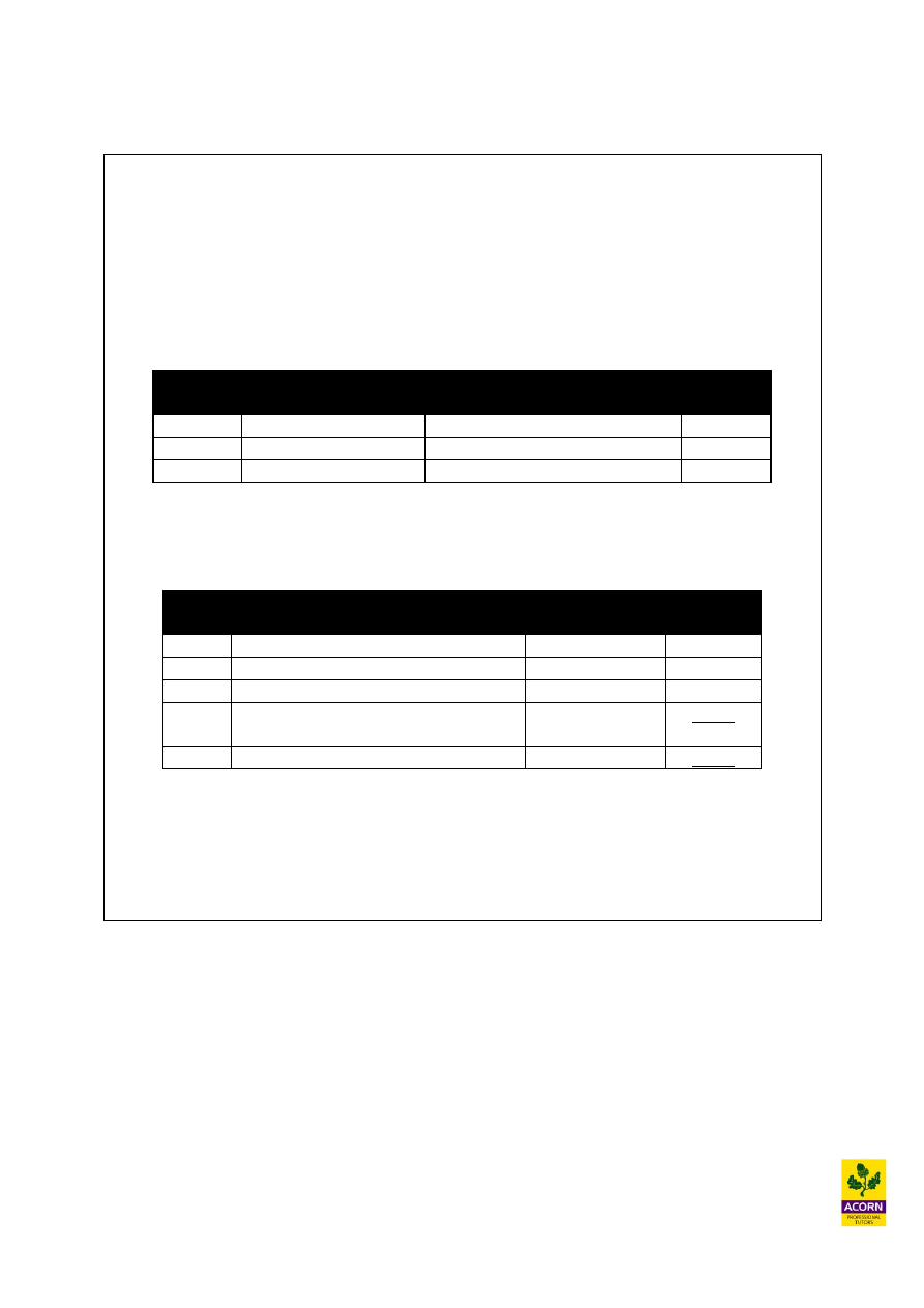
To create the initial tableau list all the slack variable on the left hand side and across the top
of the table have your remaining variables. Then layout each equality constraint as below
against the relevant slack variable constraint and then at the bottom the solution row should
be the objective function. See table below.

Variables in the
solution

A

B

p

q

r

s

Solution
column

p

3

4

1

0

0

0

9,000

q

1

2

0

1

0

0

4,000

r

0.5

0.25

0

0

1

0

1,000

s

1

0

0

0

0

1

1,200

Solution row

-8

-14

0

0

0

0

0

The next step is to carry out a series of iterations to (using a computer for more complex
tableaus) find and test each feasible point in the feasible region, and then finally a solution
would be reached as below. You do not need to know how to do these iterations.

Variables in the
solution

A

B

p

q

r

s

Solution
column

A

1

0

1

-2

0

0

1,000

B

0

1

-0.5

1.5

0

0

1,500

r

0

0

-0.375

0.625

1

0

125

s

0

0

-1

2

0

1

200

Solution row

0

0

1

5

0

0

29,000

The value of each variable is shown in the solution column. The variables in the solution
column are A, B, r and s. This would mean that p and q have zero values (all used up
completely in the solution) and therefore do not have a solution i.e. anything that has no slack
(or slack equals zero) is not shown in the solution column. To find the solution to a variables
corresponding value in the solution column, only a 1 will appear in its column with the rest of
the values being 0 e.g. ‘Bs’ column is 0 1 0 0 0. Look to the right hand side of the ‘1’ within
the solution row of ‘B’ above and the solution for the value of B in the solution column is
1,500 (indicating 1,500 units are being made).

The solution therefore is to make 1,000 units of A and 1,500 units of B. 125 units of r (the
number of unused units of material) exist and 200 units of s (the amount that demand for A
falls short of 1,200 units), r and s therefore being ‘slack resources’. The value of the
objective function (contribution) would be £29,000.

8

This therefore means that if p and q are not shown in the solution column they must be fully
used and therefore shadow prices are relevant here and displayed in the table in the solution
row (the extra contribution earned, for each extra unit of that scarce resource if you could
obtain more of it).

p (the number of unused skilled labour hours) and q (the number of unused unskilled labour
hours) are zero indicating that all labour hours regardless of skill level are being used to
maximum (hence no value for these in the solution column). The solution row shows that for
each additional hour of skilled and unskilled labour obtained at their normal variable cost per
hour, extra contribution or the shadow price that will be earned will be £1 and £5
respectively.

The solution column for p and q also shows what would happen to the variables A, B, r and s
should one more unit of p or q be obtained e.g. one more unit of p would increase the number
of units ‘A’ by 1, but the number of units ‘B’ would fall by 0.5. (the contribution increasing
by (£8 x 1) + (£14 x –0.5) = £1 ‘the shadow price of p. This would also cause a decline in ‘r’
of -0.375 (extra material used 0.5(1) + 0.25(-0.5) = -0.375 and ‘s’ of 1 unit of A, as if ‘A’
rises by 1 unit, for every additional hour obtained, then the maximum demand unfulfilled
would now be 199 rather than 200 units as before (product A produced in other words would
now be 1,001 rather than 1,000 as above in the solution).

This information therefore is useful as you could carry out a sensitivity analysis, testing how
the optimal solution would change if more or less of a scarce resource (p or q) were made
available. The information can also be used to make decisions about the maximum premium
or price that is worth paying for a scarce resource as well.

However when making decisions about p above remember the shadow price is only relevant
up to the slack or surplus that exists for r (material) and s (maximum demand for A) to the
amount of 125 units and 200 units respectively, also every extra hour of skilled labour would
also cause a fall of 0.5 of B as well. Therefore if you take p as an example in the solution
above, the shadow price will only be relevant up to either 125/0.375 (unused material) = 333
hours of p (skilled labour hours) or 200/1 (maximum demand for A) = 200 hours of p (skilled
labour hours) or 1,500/0.5 (B cannot be negative and falls by 0.5 units every extra hour of
skilled labour made available) = 750 hours of p (skilled labour hours) therefore the most
hours you would ever want for p in this case would be the lowest of the three 200 hours. You
would not want to obtain any more skilled labour than this; otherwise the solution for shadow
pricing purposes would become invalid for any further hours obtained! All of the above
analysis can also be applied to q (unskilled labour hours). If less of a scarce resource was
made available the same analysis would apply but in reverse.

9

Example 9.7

(a) In the case of unskilled labour (q) in the example above what is the most hours you could
obtain in order for its shadow price to remain valid of £5 for every extra unskilled labour
hour made available?

(b) Unskilled staff could be asked to work Sundays and therefore work an extra 400 hours a
week for the company. However staff would want to be paid £9.50 an hour rather than the
normal £6 an hour they are getting at present.

How much additional contribution would the company earn from this?

(c) The company has a trade union meeting to negotiate a new hourly rate for Sunday work
introduced. What is the maximum price the company should pay per hour, assuming the 400
extra hours of work are agreed?

(d) A temp agency has offered in total, 600 hours of unskilled labour each Sunday at £9 an
hour, but the company at this deal must take the whole 600 hours they have no choice. Is this
financially better or worse than asking current staff to work overtime at £9.50 an hour?



Example 9.8 – (CIMA past exam question)

The following equations have been taken from the plans of DX for the year ending 31
December 2005:

Contribution (in dollars) = 12x1 + 5x2 + 8x3

2x1 + 3x2 + 4x3 + s1 = 12,000 kilos

6x1 + 4x2 + 3x3 + s2 = 8,000 machine hours

0 ≤ x1 ≤ 2,000

100 ≤ x2 ≤ 500

5 ≤ x3 ≤ 200

where: x1, x2, and x3 are the number of units of products produced and sold, s1 is raw
material still available, and s2 is machine hours still available.

If an unlimited supply of raw material s1 could be obtained at the current price, what is the
product mix that maximises the value of DX plc’s contribution?

10

Key summary of chapter



Single limiting factor use “contribution per limiting factor” analysis.



Multiple limiting factors use linear programming.

Shadow pricing



Only relevant if a limiting factor exists.



It is the extra contribution gained by obtaining one more unit of the limiting factor.



Maximum price = shadow price + cost per unit of limiting factor.

Linear programming

It can be applied in several different situations:



Mix of materials in products



Capacity allocation



Distribution problems



Production forecasting



Investment mix



Logistical problems

Approach to answering linear programming questions



Define variables.



Construct the objective function (maximise contribution).



Set up the constraints (don’t forget to include the non-negativity constraints).



Solve through graphical method or simultaneous equations.

11

Solutions to lecture examples

12

Chapter 9

Example 9.1

1000

1200

2000

Chips

Fish

C = 3/2F

0.08F + 0.04C = 48

0.1F + 0.05C = 100

F = 500

514

343

500

A

1000

1200

2000

Chips

Fish

C = 3/2F

0.08F + 0.04C = 48

0.1F + 0.05C = 100

F = 500

514

343

500

A

1000

1200

2000

Chips

Fish

C = 3/2F

0.08F + 0.04C = 48

0.1F + 0.05C = 100

F = 500

514

343

500

A

1000

1200

2000

Chips

Fish

C = 3/2F

0.08F + 0.04C = 48

0.1F + 0.05C = 100

F = 500

514

343

500

A

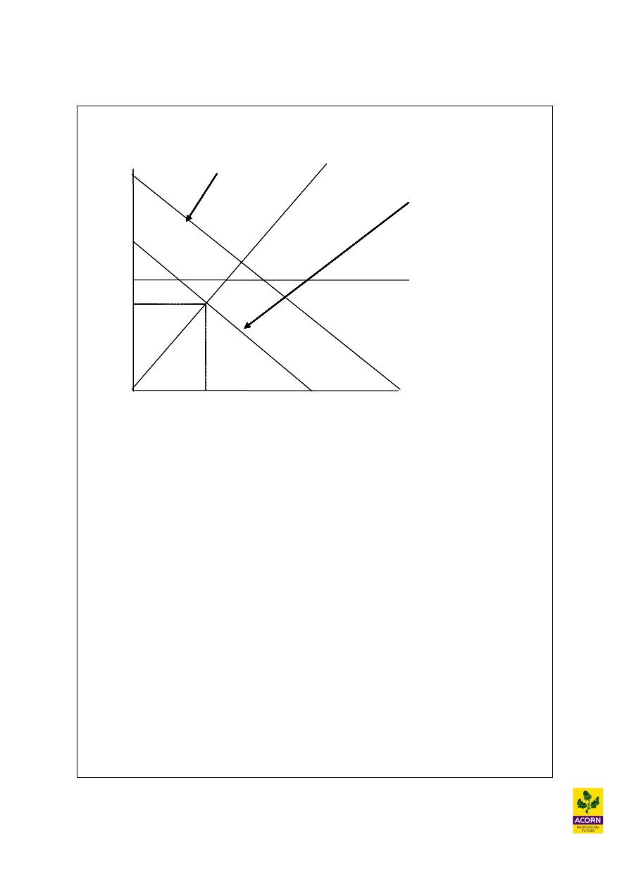
The feasible area for production has to be on or behind the cooking time constraint, but
due to the manager asking staff to cook 3 portions of chips for every 2 portions of fish,
production must be on this line at all times for the constraint C = 3/2F or F = 2/3C.

To maximise contribution therefore production will be at the point where cooking time
and the production mix constraint intersect one another – point A.

Reading from the graph this will be 514 chips and 343 fish producing contribution of:

1.5 (343) + 0.50 (514) = £771.50

This solution can also be solved using simultaneous equations as at point A using both
constraint lines the number of fish and chips in each of the two equations will be exactly
the same (as both equation lines are on the same point.

1

0.08F + 0.04C = 48

2

C = 3/2F

3

0.08F + 0.04(3/2F) = 48

4

0.08F + 0.06F = 48

5

0.14F = 48

6

F = 48/0.14

7

F = 343

Therefore if C = 3/2F then C = 3/2(343) = 514

13

Example 9.2

1000

1200

2000

Chips

Fish

0.08F + 0.04C = 48

0.1F + 0.05C = 100

F = 500

200

500

A

1000

1200

Fish

0.08F + 0.04C = 48

0.1F + 0.05C = 100

F = 500

200

500

A

1000

1200

2000

Chips

Fish

0.08F + 0.04C = 48

0.1F + 0.05C = 100

F = 500

200

500

A

1000

1200

Fish

0.08F + 0.04C = 48

0.1F + 0.05C = 100

F = 500

200

500

A

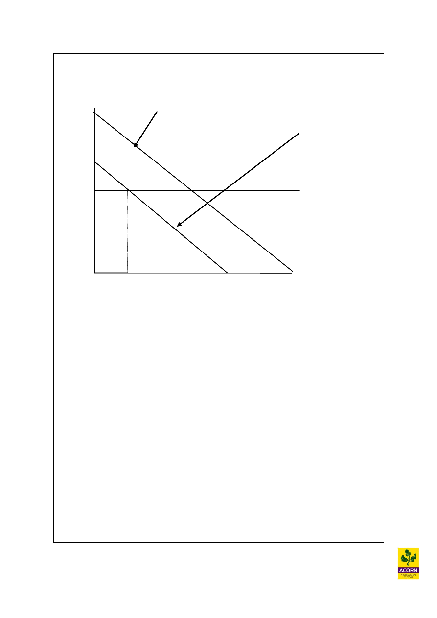
Now that the manager has relaxed the production mix constraint, it is again the cooking
time but also this time the EU regulation that are the two binding constraints. The
production points are always where a line intersects the Y or X axis on a graph or where
two lines intersect one another.

Possible production points could be where F = 500 and no chips produced (contribution
500 x 1.50 = £750) also where C = 1200 and no fish are produced (contribution 1200 x
0.50 = £600)

However in this case the furthest most point from the origin would be where C = 200 and
F = 500 as this will generate the most contribution (1.5 (500) + 0.50 (200) = £850)

Proof:

At point A the number of fish and chips in the following equations are equal to one
another therefore solve

1. F = 500
2. 0.08F + 0.04C = 48
3. 0.08(500) + 0.04C = 48
4. 40 + 0.04C = 48
5. 0.04C = 8
6. 8/0.04 = 200

14

Example 9.3

Variables in the
solution

A

B

p

q

r

s

Solution
column

A

1

0

1

-2

0

0

1,000

B

0

1

-0.5

1.5

0

0

1,500

r

0

0

-0.375 0.625

1

0

125

s

0

0

-1

2

0

1

200

Solution row

0

0

1

5

0

0

29,000

Every extra hour obtained for unskilled labour time (q) gives a decline of –2 product A
(hence maximum demand slack will rise by 2), however would also cause B, r and s to
increase, therefore these constraints are not a problem (unless of course we were reducing
the unskilled labour time available – the situation explained would be in reverse).

Therefore 1,000/2 for ‘A’ above (The number of units of product A cannot be less than
zero so cannot fall below 1,000) = 500 extra hours of unskilled labour time could be
made available for the shadow price of q to remain valid.

An overtime premium would be worth it.

400 hours of skilled labour x (£5 shadow price - £3.50 overtime premium) = extra
contribution earned of £600.

The maximum price for the 400 extra hours would be £6 normal rate (already deducted in
the contribution solution when calculating the shadow price) + shadow price £5 = £11 an
hour.

600 hours from a temp agency at £9 an hour?

Only 500 hours could be used (as once 500 hours is exceeded something else becomes the
scarce resource other than ‘q’. In this case it would be Product A, as this falls to zero at
500 hours. Therefore the additional 100 hours could not be used.

500 x £5 (shadow price of q) = £2,500
500 x (£9-£6 normal cost*) = (£1,500)
100 x £9 = (£900)
Extra contribution £100

* normal cost already deducted in arriving at the shadow price

The 100 hours above would be paid for, but no extra contribution would have been
earned. This therefore is not financially viable as asking current staff to work Sundays
(£600 extra contribution earned in this case rather than only £100 as above.

15

Example 9.4 – (CIMA past exam question)

If “s1” becomes unlimited being raw material then the other resource machine hours must
still be limited as we have not been told otherwise.

Therefore we can make as much as we like of “x1”, “x2” and “x3” but will be limited by
machine hours at some point. Therefore we should produce those products which give us the
most contribution per limiting factor being machine hours in this instance.

Products

Contribution per

unit

Contribution per machine

hour

Ranking

x1

$12

$12 / 6hrs = $2 per hour

2

x2

$5

$5 / 4hrs = $1.25 per hour

3

x3

$8

$8 / 3hrs = $2.67 per hour

1

The question says before we can make what we like in accordance to our rankings we must
make sure we produce the minimum quotas for “x2” and “x3” of 100 units and 5 units
respectively.

Make

Machine

hrs used

x2

Minimum 100 units x 4hrs =

400

x3

Minimum 5 units x 3hrs =

15

x3

195 units x 3 hrs =

585

x1

8,000hrs – 400hrs – 15hrs – 585hrs
= 7,000hrs

7,000hrs / 6hrs
= 1,166 units

7,000

8,000

Summary of products made:

“x1” = 1,166 units
“x2” = 100 units
“x3” = 195 units + 5 units = 200 units