SAE 950417

Automotive Engine Modeling for

Real-Time Control Using

M

ATLAB

/S

IMULINK

Robert W. Weeks

Modular Systems

John J. Moskwa

Powertrain Control Research Laboratory

University of Wisconsin-Madison

SAE 950417 Weeks & Moskwa 3/24/95

-1-

This paper was published and presented at the Society of Automotive Engineers
1995 International Congress and Exposition, Detroit, MI.

For more information you can contact:

Phone: Internet:

SAE [phone]
Robert Weeks [phone] [e-mail]

http://www.simcar.com

John Moskwa [phone] [e-mail]

ABSTRACT

The use of graphical dynamic system simulation software

is becoming more popular as automotive engineers strive to
reduce the time to develop new control systems. The use of
model-based control methods designed to meet future emission
and diagnostic regulations has also increased the need for
validated engine models. A previously validated, nonlinear,
mean-torque predictive engine model

*

is converted to

M

ATLAB

/ S

IMULINK

†

to illustrate the benefits of a graphical

simulation environment. The model simulates a port-fuel-
injected, spark-ignition engine and includes air, fuel and EGR
dynamics in the intake manifold as well as the process delays
inherent in a four-stroke cycle engine. The engine model can
be used in five ways:

•

As a nonreal-time engine model for testing engine control
algorithms

•

As a real-time engine model for hardware-in-the-loop
testing

•

As an embedded model within a control algorithm or
observer

•

As a system model for evaluating engine sensor and
actuator models

•

As a subsystem in a powertrain or vehicle dynamics model

Although developed and validated for a specific engine,

the model is generic enough to be used for a wide range of
spark-ignition engines. Modular programming techniques
reduce model complexity by dividing the engine and control
system into hierarchical subsystems.

*

Developed under a contract from the Power Systems

Research Department of General Motors Research
Laboratories.

†

M

ATLAB

and S

IMULINK

are trademarks of The

MathWorks, Inc.

INTRODUCTION

Dynamic system simulation software is an important tool

for developing reliable, low emission engine and powertrain
control systems. Several companies market software (and
hardware) that can be used to rapidly simulate a dynamic
system and its controller using various combinations of PC
and/or workstation technology.

‡

Many of these companies

provide software tools that allow development of libraries of
component models. As these component model libraries are
developed, new control systems are easily simulated by
reusing previously built subsystems.

In an effort to develop some of these reusable subsystem

models, a previously validated mean torque predictive engine
model was converted from FORTRAN to M

ATLAB

/

S

IMULINK

.

§

The S

IMULINK

engine model is simulated

within a larger system model that also includes sensor, actuator
and engine controller subsystem models.

The paper begins with an overview of the engine and

control system model briefly describing the various
subsystems. Additional detail is provided for the engine
model’s intake manifold subsystem before a series of example
simulations are examined. The example simulations illustrate
how mean torque predictive models can be useful for
predicting a number of variables important to the control
system engineer. Execution times for the model are provided
in the appendix.

‡

A partial list includes: The MathWorks, Inc., Integrated

Systems, Inc., dSPACE GmbH, Xanalog Corp. and Visual
Solutions, Inc.

§

A complete theoretical review of the mean torque

predictive engine model is beyond the scope of this paper.
Readers interested in a detailed development of the engine
model should refer to [1,2,3].

SAE 950417

Weeks & Moskwa 3/24/95

-2-

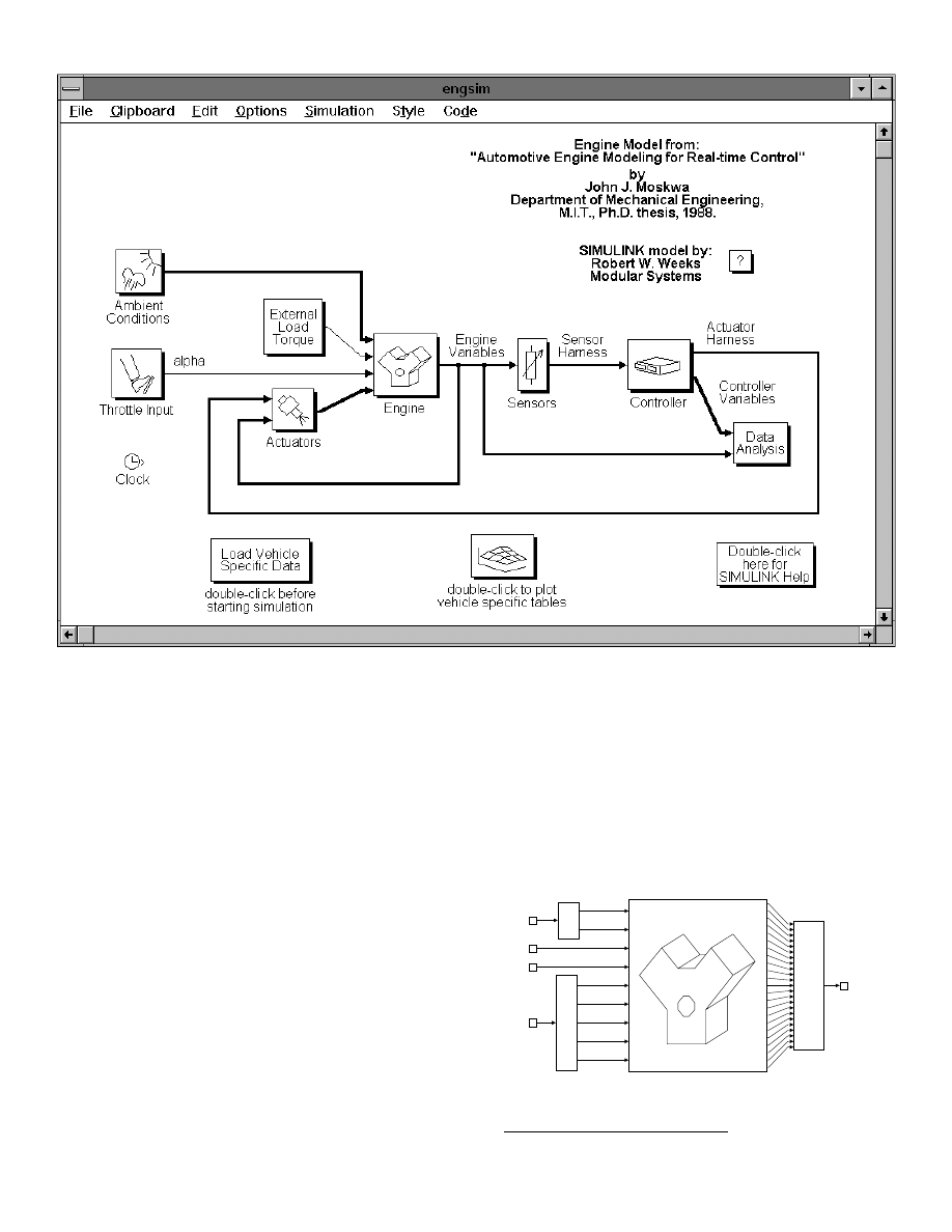
Figure 1: Root level of the S

IMULINK

engine and control system model

ENGINE AND CONTROL SYSTEM MODELS

This section briefly describes the uppermost (or “root”)

level of the engine and control system model shown in Fig. 1.
This level of the model is displayed when the file “engsim.m”
is loaded into S

IMULINK

. The S

IMULINK

graphical block

diagram language allows models to be written in a modular,
hierarchical format. The overall system model in Fig. 1
simulates an engine and control system consisting of an
engine, engine sensors and actuators and an engine controller.
Inputs to the engine include: throttle angle, an external load
torque such as that due to a dynamometer or a transmission,
ambient conditions (i.e., atmospheric temperature and
pressure) and actuator inputs from various “actuators” such as
fuel injectors, EGR valve, etc. All the important engine
variables are “vectored” and made available to other
subsystems such as Sensors, Actuators and Data Analysis.
Before a simulation is run the Load Vehicle Specific Data
block must be double-clicked with a mouse. This executes an
m-file script which loads all of the vehicle specific parameters
into M

ATLAB

’s workspace memory. By separating vehicle

specific data from the subsystem models, the models are more
generic, allowing development of one model that simulates
several engines.

Engine

The inside of the Engine block (from Fig. 1) is shown

below in Fig. 2. This block “demuxes” all the engine’s inputs
and routes them into the Mean Torque SFI Engine block.
The Mean Torque SFI Engine block contains a S

IMULINK

version of the engine model described in [1]. All the
important variables from the engine model are routed into the
Engine Variable Connector where they are “muxed” into a
vector

*

called Engine Variables.

mdot_fi

3

alpha

2

Tload

1

Ambient

Conditions

Pin

Tin

4

Actuator

Outputs

Demux

Demux

spark_advance

inj_pw_deg

mdot_IAC

mdot_egri

Demux

Demux1

Mean Torque SFI Engine

Engine

Variable

Connector

1

Engine

Variables

Figure 2: Engine block (from Fig. 1)

*

Vectors in S

IMULINK

1.3 are normally shown as thick

lines in block diagrams.

SAE 950417

Weeks & Moskwa 3/24/95

-3-

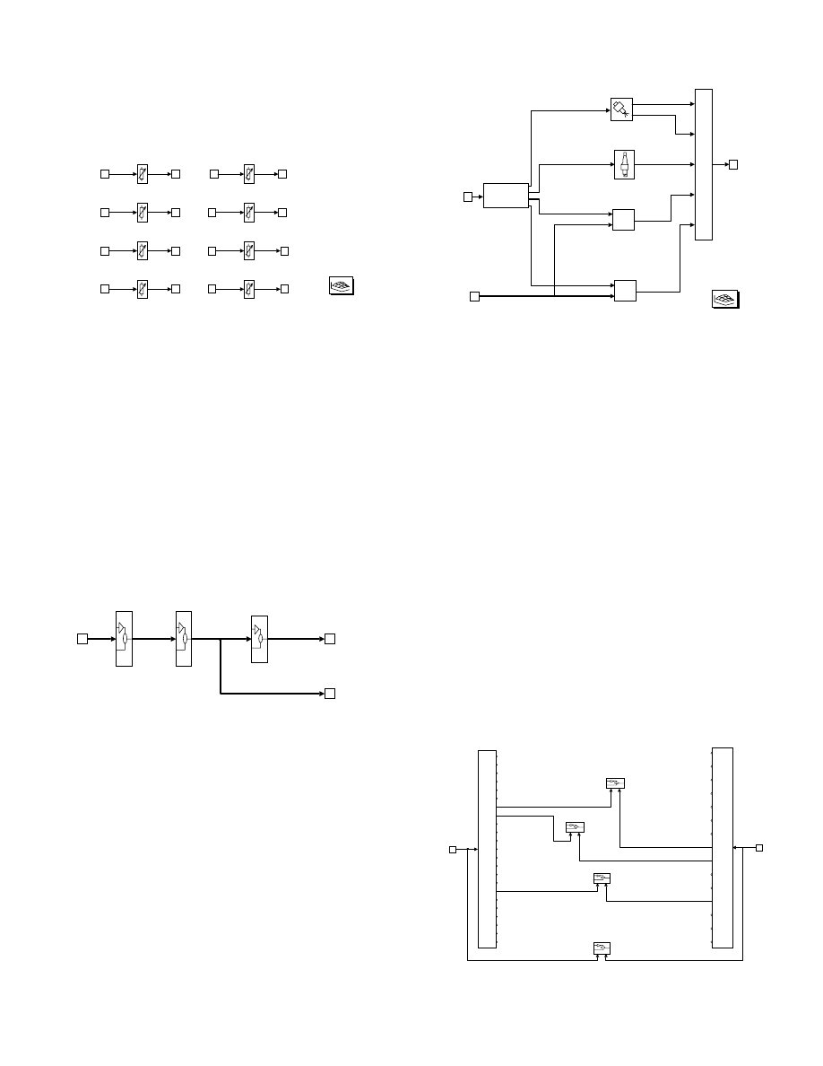
Sensors

The Sensors block visible in Fig. 1 contains all the engine

sensor models (shown in Fig. 3). A subset of the engine
variables are routed into individual sensor models. Each
sensor may be modeled to the degree of accuracy necessary for
a given simulation.

7

out_7

8

out_8

4

out_4

5

out_5

3

out_3

6

out_6

2

out_2

1

out_1

8

in_8

7

in_7

6

in_6

5

in_5

4

in_4

3

in_3

2

in_2

1

in_1

double-click to plot

sensor tables

Engine Speed

Sensor

Ambient Air

Temperature Sensor

Manifold Absolute

Temperature Sensor

Air Mass

Sensor

Baro Sensor

Manifold Absolute

Pressure Sensor

Throttle Position

Sensor

Exhaust Gas

Oxygen Sensor

Figure 3: Sensors block (from Fig. 1)

Controller

The contents of the Controller block shown in Fig. 1 are

shown below in Fig. 4. Discrete time control algorithms are
placed inside the Control Algorithms block which is “wired”
between the input and output signal conditioning blocks. The
Input Signal Conditioning block performs the conditioning
necessary to convert the simulated sensor outputs to the
engineering units typically used by the Control Algorithms
block. This often involves analog-to-digital converter models
and conversion tables. The Output Signal Conditioning
block converts control signals to the type of signal necessary
for the engine’s control actuators, such as a pulse width
modulated signal, a desired stepper motor position, etc.

1

Sensor

Outputs

Controller

Variables

Digitized

Inputs

Input Signal

Conditioning

Control

Algorithms

Output Signal

Conditioning

1

Actuator

Inputs

2

Controller

Variables

Figure 4: Controller block (from Fig. 1)

Actuators

The contents of the Actuators block (from Fig. 1) are

shown below in Fig. 5. Four actuators are used for this engine
control system, including fuel injectors, an ignition system, an
exhaust gas recirculation valve and an idle air control valve.
The actuator commands (from the controller) come in through
inport 1. A Signal Select block was created to split the
actuator signal vector (or “harness”) and route the signals to
the appropriate actuator models. Each of the actuators has a
mass flow rate for its output, except for the Ignition System
block where the output is simply a value for the current spark
advance. The Fuel Injectors block also determines the
injector pulse width in degrees of crank rotation. This is used
in the engine model to determine if a portion of the fuel pulse

is injected after the intake valve closes (and thus goes through
an additional delay before entering the cylinder).

IAC_cmd

mdot_IAC

IAC

Valve

EGR

Valve

Ignition System

Fuel Injectors

mdot_fi

inj_pw_deg

spark_adv

double-click to plot

actuator tables

2

Engine

Variables

SA_cmd

mdot_fi_cmd

EGRvalve_cmd

Mux

Mux

1

mdot_egri

Signal Select

(using mux)

1

Actuator

commands

Figure 5: Actuators block (from Fig. 1)

The mass flow rates through the EGR and IAC valves are

affected by the stagnation conditions upstream of the valves as
well as the pressure drop across the valves. These two valve
models are therefore connected to the Engine Variables
vector allowing access to the appropriate pressures and
temperatures from the engine model. Separating the actuator
models from the engine model allows revisions (or
substitutions) of the actuator models without updating the
engine model. This type of modularity makes the engine
model more generic.

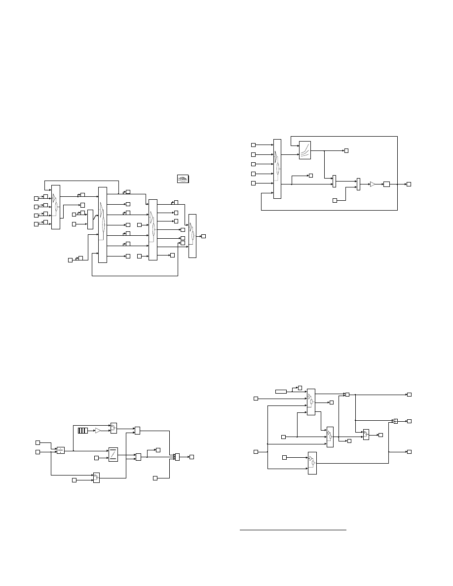
Data Analysis

The contents of the Data Analysis block (from Fig. 1) are

shown below in Fig. 6. This block is used strictly for storing
data to the M

ATLAB

workspace (or to disk) as well as for

visualizing variables during a simulation run (typically with
S

IMULINK

scope blocks). The Data Analysis block can be

removed from the overall control system model without
affecting the simulation. It simply provides a convenient
method for comparing variables in the engine to variables in
the controller. Engine and controller variable vectors are
“demuxed” in the Data Analysis block to make it easy to
select arbitrary combinations of variables for visualization
during a simulation run.

1

Controller
Variables

14 mdot_throt

Demux

Demux1

20 Texh

3 AFport

23 torq_fric_pump

22 torq_indicated

21 Tman

19 Tcool

18 Tamb

17 Pman

16 Pexh

15 Pamb

13 mdot_IAC

12 mdot_fo

11 mdot_fi

10 mdot_egro

9 mdot_egri

8 mdot_ao

7 mdot_ai

6 EngSpeed

5 EGRfrac

4 alpha

2 AFexh

1 AFego

Demux

Demux

2

Engine

Variables

Tman_m 25

Tamb_m 14

SA_cmd 13

IAC_cmd 7

EGRvalve1_cmd 5

EGRvalve2_cmd 4

alpha_m 2

AFego_m 1

EngSpeed_m 6

EGRvalve3_cmd 3

mdot_fi_cmd 10

Pamb_m 11

Pman_m 12

mdot_AMS_m 8

mdot_ao_est 9

display throttle

flow rates

display

pressures

Save Results

display port

flow rates

Figure 6: Data Analysis block (from Fig. 1)

SAE 950417

Weeks & Moskwa 3/24/95

-4-

MEAN TORQUE SFI ENGINE MODEL

The Engine block briefly described in the previous

section is more thoroughly described in this section. The
engine model is physically based and captures the major
dynamics (lags and delays) inherent in the spark ignition
torque production process. It is a continuous time delay, mean
torque-predictive model designed primarily for the control
engineer. It does not attempt to predict flow and torque
pulsations due to individual cylinder filling events. The engine
model was derived from the four state, lumped parameter
dynamic engine model developed in [1].

The Mean Torque SFI Engine block (from Fig. 2) is

shown below in Fig. 7. This block consists of four subsystem
blocks: the Throttle Body, the Intake Manifold, the Engine
Block and the Exhaust Manifold.

mdot_ai

7

mdot_throt

14

11

Mux

Mux

5

mdot_fi

6

inj_pw_deg

Throttle Body

13

18

15

4

2

Tamb

1

Pamb

4

alpha

9

mdot_IAC

9

8

mdot_egri

2

EngSpeed

torq_indicated

Texh

Tcool

AFexh

16

1

AFego

Pexh

6

20

19

22

torq_fric_pump

Exhaust

Manifold

23

Engine

Block

7

spark_adv

3

Tload

10

5

3

12

8

21

17

mdot_egro

EGRfrac

AFport

mdot_fo

mdot_ao

Tman

Pman

Intake

Manifold

double-click to plot

engine specific tables

Figure 7: Mean Torque SFI Engine block (from Fig. 2)

The Throttle Body block calculates the total mass flow

rate of air entering the intake manifold (mdot_ai). One-
dimensional isentropic compressible flow equations determine
the throttle flow rate (mdot_throt) as a function of throttle
angle (alpha), intake manifold pressure (Pman), and upstream
stagnation conditions (Pamb and Tamb). The total flow rate
into the manifold is simply the sum of the throttle flow rate,
the idle air control valve flow rate, and the flow due to any
intake manifold leaks as shown below in Fig. 8. The throttle
flow rate calculations used in the throttle body model have
also proven useful in engine controllers for constructing
“observers” that estimate the transient air flow rate at the
throttle and intake ports of an engine [4].

P and T Correction

*

Product

*

Product1

Vacuum Leak

Flow

+

+

+

Sum

1

mdot_ai

4

Tamb

2

mdot_throt

mdot_leak

2

alpha

Throttle Flow

5

mdot_IAC

-K-

Leak

Size

divide

1

Pman

3

Pamb

PR

Repeating
Sequence

Figure 8: Throttle Body block (from Fig. 7)

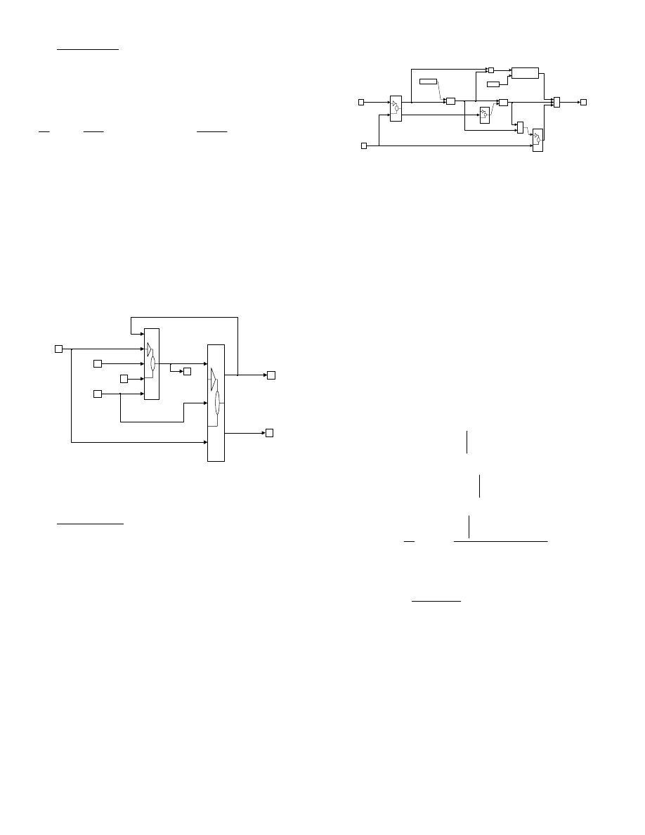
The Intake Manifold block’s main purpose is to

determine the manifold pressure as well as the mean-value
mass flow rates of air, fuel and EGR in the intake ports of the
engine. A more complete description is given in the Intake
Manifold subsection that follows.

The Engine Block’s main purpose is to perform the

torque production and rotational dynamics calculations.
Double clicking two levels down into the Engine Block block
reveals the Torque Production block shown below in Fig. 9.
The Torque Production block calculates the indicated torque
(torq_indicated) and subtracts off the friction and pumping
torque of the engine (torq_fric_pump) to get the brake torque
(torq_brake). Any external load torques are then subtracted
from the brake torque to determine the net torque which
accelerates or decelerates the crankshaft. The crankshaft
acceleration is then integrated to get the engine speed
(EngSpeed).

1/s

Integrator

Friction and

Pumping

Torque (tbl)

EngLoad

1

torq_indicated

2

torq_fric_pump

5

Load torque

torq_brake

3

EngSpeed

-K-

1/Je

+

-

Net torque

-

+

Sum

Calculate

Indicated Torque

2

Pman

1

EGRfrac

6

spark_adv

4

AFport

3

mdot_ao

Figure 9: Torque Production block

Intake Manifold

The Intake Manifold block (mentioned earlier in the

MEAN TORQUE SFI ENGINE MODEL section) is more
thoroughly examined in this subsection to lay the groundwork
for a parametric study presented later in the EXAMPLE
SIMULATIONS section of the paper. The contents of the
Intake Manifold block from Fig. 7 are shown below in Fig.
10. The intake manifold has three dynamic subsystems: air,
fuel and EGR. The Air Dynamics block calculates a port flow
rate which assumes a homogeneous mixture of air and EGR.
The port EGR flow rate (mdot_egro) is then subtracted from
the total port flow rate (air + EGR) to determine the port air
flow rate (mdot_ao). The port fuel flow rate (mdot_fo) is
assumed to not interact with the air or EGR dynamics.

*

An

intake port air/fuel ratio is calculated by simply dividing the
port air flow rate by the port fuel flow rate.

1

Pman

+

-

Sum

EGR

Dynamics

Air

Dynamics

4

mdot_fo

3

mdot_ao

EGR

fraction

6

EGRfrac

divide

5

AFport

7

mdot_egro

1

mdot_ai

Tman
Tman

2

3

mdot_egri

4

EngSpeed

Fuel

Dynamics

2

mdot_fi and

inj_pw_deg

VE

Figure 10: Intake Manifold block (from Fig. 7)

*

On gasoline engines the partial pressure of fuel vapor in

the intake manifold can generally be ignored in regards to its
affect on air or EGR flow.

SAE 950417

Weeks & Moskwa 3/24/95

-5-

Air Dynamics
The contents of the Air Dynamics block from Fig. 10 are

shown below in Fig. 11. The Manifold filling dynamics
block (from Fig. 11) calculates the intake manifold pressure
(Pman) using a block diagram version of Eq. 1 [1]:

d

dt

P

T

T

C

P

R T

V

m

m

man

man

man

e

vol

man

man

man

ai

egri

=

− ⋅

⋅

F

HGG

I

KJJ

⋅

+ ⋅

⋅

+

FH

IK

•

•

•

1

ω η

. (1)

The Port flow rate block in Fig. 11 determines the total port
flow rate using a speed-density calculation. The model
assumes air and EGR are homogeneously mixed and have the
same molecular weight and temperature. With this
simplification it is possible to estimate the combined mass
flow rate of air and EGR entering the cylinders using a
traditional speed-density calculation. In practice, it is difficult
to determine the percentage of the combined flow rate due to
air flow alone (mdot_ao). In the model this value is calculated
by subtracting the EGR flow (mdot_egro) from the combined
flow (see Fig. 10).

2

Pman

1

Total port

flow rate

3

VE

2

mdot_ai

4

mdot_egri

3

EngSpeed

1

Tman

Manifold filling

dynamics

Port

flow rate

Figure 11: Air Dynamics block (from Fig. 10)

Fuel Dynamics
The contents of the Fuel Dynamics block visible in Fig.

10 are shown below in Fig. 12. The calculations performed in
the Fuel Dynamics block are based on Eqs. 2-6 below [1,3]. A
fraction of the mean injector flow rate (shown as mdot_fi in
Fig. 12), goes through one or two pure time delays as well as a
first order lag before it finally enters the cylinders as mdot_fo.
The pure time delay, t

T

− ∆

1

b

g

, represents the average delay

from a change in the fuel command to the actual start of
injection (SOI) plus the delay from the start of injection until
the intake valve closes (IVC). This delay is performed by the
fuel delay (delta t1) block in Fig. 12. The delay, t

T

− ∆

2

b

g

,

represents a two revolution delay for any fuel injected after the
intake valve closes (see the 2 rev delay (delta t2) block in
Fig. 12).

epsilon and tauf are shown as constants here but in general

are time varying functions of speed, load, temperature, etc.

if intake valve closes while fuel is injected

then some fuel gets delayed two revs

2

EngSpeed

2 rev delay

(delta t2)

fuel delay

(delta t1)

gamma

-
+

Sum1

slow fuel

mdot_fs1

tauf

slow fuel

time constant

epsilon

fuel split

1

mdot_fi

and

inj_pw_deg

*

Product1

fast fuel

+

-

Sum

Time varying

Lag filter

Slow fuel lag

mdot_ff2

*

Product

1

mdot_fo

+

+

+

Sum2

mdot_ff3

Figure 12: Fuel Dynamics block (from Fig. 10)

The fuel split parameter,

ε

, is the fraction of the injected

fuel with transport properties of a gaseous fuel. It is called
“epsilon” in Fig. 12. The slow fuel time constant,

τ

f

, is the

first order lag filter time constant applied to the fraction of the
injected fuel with transport properties of a liquid fuel. It is
called “tauf” in Fig. 12. The variable,

γ

, is the fraction of the

fuel injected before the intake valve closes. It is calculated
and output from the gamma block in Fig. 12. The values of
“epsilon” and “tauf” are shown as constants in Fig. 12, but in
general are time varying as a function of manifold temperature,
pressure and engine speed. A table of values could easily be
substituted for the constants in Fig. 12.

m

m

m

m

fo

ff

ff

fs

•

•

•

•

=

+

+

2

3

1

(2)

where:

m

m

ff

fi

t

T

t

T

•

•

−

−

=

⋅ ⋅ −

L

NM

O

QP

2

1

2

1

∆

∆

b g

b

g

b g

ε

γ

(3)

m

m

ff

fi

t

T

•

•

−

=

⋅ ⋅

3

1

∆

b g

ε γ

(4)

d

dt

m

m

m

fs

fi

t

T

fs

f

•

•

−

•

FH IK

=

⋅ − −

1

1

1

1

∆

b g

a f

ε

τ

(5)

γ =

≤

>

R

S|

T|

1, if

-

-

, if

-

Φ

Φ

Φ

Φ

Φ

Φ

Φ

Φ

Φ

PW

IVC

SOI

IVC

SOI

PW

PW

IVC

SOI

(6)

ENGINE SPECIFIC TABLES

Before an engine simulation is run, the M

ATLAB

workspace memory must be loaded with all the parameters that
are specific to a particular engine. This is usually done by
double-clicking on the Load Vehicle Specific Data block in
Fig. 1 but can also be done by just typing “simspec” at the
M

ATLAB

prompt. Both methods run an m-file script called

“simspec.m”. This m-file actually executes a number of other
m-files which all contain data specific to one or more of the
subsystem models. A partial listing of simspec.m follows:

SAE 950417

Weeks & Moskwa 3/24/95

-6-

...

% load ambient conditions

ambspec

% load engine specs and initialization values

engspec

% load sensor specs

sensspec

% load controller specs

ctrlspec

% load actuator specs

actspec

% load disturbance specs (noise, leaks, etc.)

distspec

...

Each of the commands above executes a script file; for

example “ambspec” executes the script file ambspec.m which
initializes the variables used for ambient temperature and
pressure. Tables are used for many of the engine specific
parameters even if an analytical expression could have easily
been embedded in the S

IMULINK

model.

*

Tables make the

model more generic because they have more degrees of
freedom than an analytical expression or regression equation.
In some cases tables are initialized using regression equations.
This gives additional flexibility without the need to embed
engine specific equations in the S

IMULINK

model.

In addition to initializing a number of engine specific

constants such as engine displacement (Veng) and intake
manifold volume (Vman), the m-file engspec.m loads nine
engine specific tables of the following parameters:

•

Throttle characteristic vs. throttle angle

•

Pressure ratio influence vs. pressure ratio

•

Volumetric efficiency vs. engine speed and manifold
pressure

•

MBT spark vs. engine speed and load

•

Air/fuel ratio influence vs. air/fuel ratio

•

Spark influence vs. spark advance relative to MBT

•

EGR correction to MBT vs. EGR fraction

•

Fuel conversion efficiency vs. engine speed and manifold
pressure

•

Friction and pumping torque vs. engine speed and load

The m-file actspec.m loads three more tables specific to

the engine actuators:

•

Fuel flowrate vs. injector pulse width

•

EGR flow calibration vs. EGR valve position

•

IAC flow calibration vs. IAC valve position

The overall accuracy of the engine model depends to a

large extent on the number of the above tables calibrated to
represent the engine of interest. The model was originally
validated using a naturally aspirated, sequential port fuel
injected, 3.8L V6 gasoline engine. Similar engines may be

*

S

IMULINK

has built-in blocks for performing table look-

ups that interpolate between table values.

simulated with reasonable accuracy without the need to
recalibrate all of the above tables.

EXAMPLE SIMULATIONS

Several simulations were run to demonstrate the output of

the engine and control system model. Unless otherwise
specified the following simulation parameters were used:

•

Engine displacement (Veng)=3.8L

•

Intake manifold volume (Vman)=3.4L

•

Fuel split parameter (epsilon)=0.53 (unitless)

•

Slow fuel time constant (tauf)=0.22 seconds

•

Discrete controller time step (deltaT)=0.005 seconds

•

Air-mass sensor time constant (AMStau)=0.005 seconds

•

Analog to Digital Converter (ADC) resolution=8 bits

(except for a 10 bit throttle angle measurement)

•

Noise on ADC inputs=

±

1

2

bit

•

Start of injection to intake valve close angle
(SOItoIVC_deg)=312 crank degrees

The throttle trajectory used for the example simulations is

shown in Fig. 13. After one second the throttle is ramped from
5 to 20 degrees at a rate of 900 degrees/second. At the two
second simulation time the throttle is ramped back to 5
degrees. No external load torques are applied to the engine, so
the simulation approximates a free-revving engine’s response
to a rapid throttle transient.

0

1

2

3

4

5

0

10

20

30

40

50

60

70

80

Time (sec)

T

h

ro

tt

le

A

n

g

le

(d

e

g

re

e

s

)

Figure 13: Throttle trajectory for example simulations

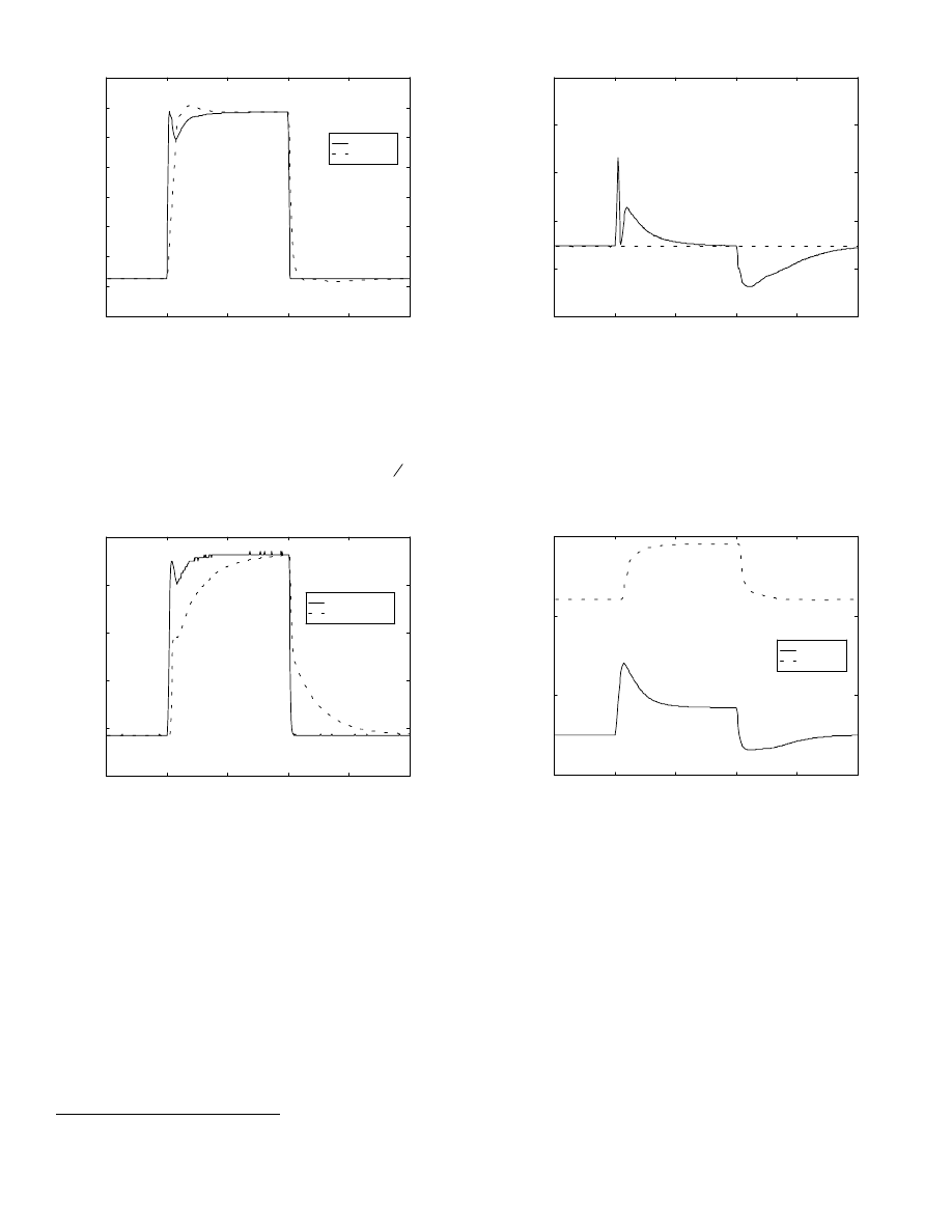
Baseline using Air Mass Sensor

Figures 14-19 illustrate the output of the engine and

control system model when an air mass sensor is used by the
controller to calculate a fuel command. Throttle and intake
port air flow rates (mdot_ai and mdot_ao, respectively) are
illustrated in Fig. 14. Note that a small manifold filling spike
appears in the throttle flow rate as the throttle is opened.

SAE 950417

Weeks & Moskwa 3/24/95

-7-

Throttle

Port

0.5

1

1.5

2

2.5

3

0

0.01

0.02

0.03

0.04

0.05

0.06

0.07

0.08

A

ir

fl

o

w

ra

te

(kg

/s

)

Time (sec)

Figure 14: Throttle and intake port air flow rates

Injector flow rate (mdot_fi) and intake port fuel flow rate

(mdot_fo) are both shown in Fig. 15. The granularity of the
injector flow rate is due to the 8 bit analog to digital converter
used to “measure” the air mass sensor as well as

±

1

2

bit of

noise included in the ADC model. The lag in the intake port
flow rate is due to the fuel dynamics, described earlier.

Injector

Intake Port

0.5

1

1.5

2

2.5

3

0

1

2

3

4

5

x 10

-3

F

u

e

l

fl

o

w

r

a

te

(

k

g

/s

)

Time (sec)

Figure 15: Injector and intake port fuel flow rates using an air-

mass sensor fuel calculation

The air/fuel excursions in Fig. 16 show that the lags due to

fuel dynamics are not canceled by the lead information
provided by the air mass sensor. The combination of the two
still results in a lean excursion due to throttle openings and a
rich excursion when the throttle closes.

*

*

On some port fuel injected engines with large intake

manifolds it is possible for the lead information from the air
mass sensor to cause a rich excursion on throttle openings.

0.5

1

1.5

2

2.5

3

0

10

20

30

40

50

In

ta

k

e

P

o

rt

A

/F

Time (sec)

Figure 16: Intake port air/fuel ratio using an air-mass sensor

fuel calculation

Intake and exhaust manifold absolute pressures are shown

in Fig. 17. The intake manifold pressure drops below 53 kPa
as the simulation time exceeds 1.25 seconds. This causes the
flow rate at the throttle to choke and thus not increase even as
engine speed rises.

Intake

Exhaust

0.5

1

1.5

2

2.5

3

0

50

100

150

M

a

n

if

o

ld

pr

ess

u

re

(

k

Pa)

Time (sec)

Figure 17: Intake and exhaust manifold absolute pressures

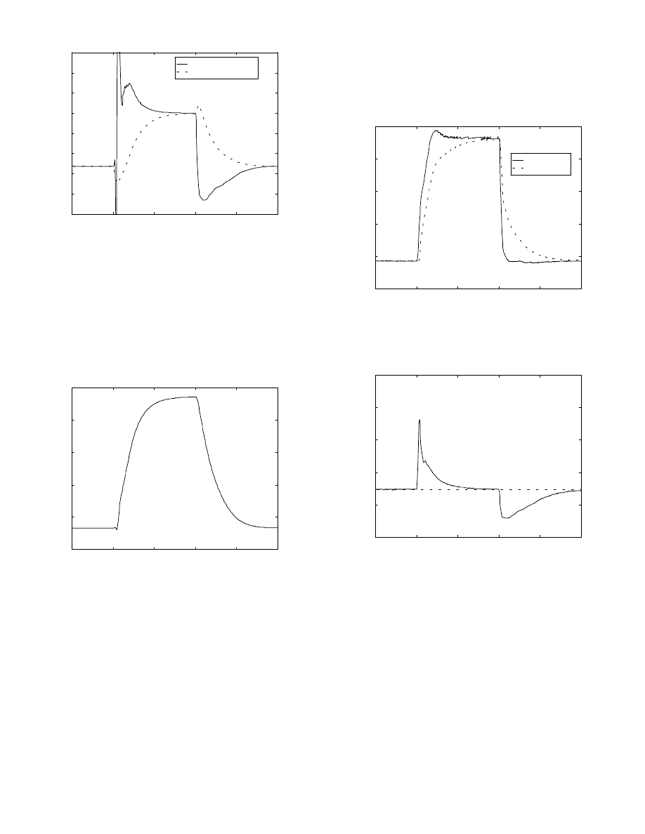
The engine’s indicated torque is plotted in Fig. 18 along

with the value of its friction and pumping torque. The initial
throttle tip-in causes an air/fuel excursion lean enough to result
in a “misfire” where indicated torque momentarily drops to
zero. As engine speed increases, the internal friction and
pumping torque of the engine approaches the value of the
indicated torque causing engine speed to level off because
there is no net torque available to continue accelerating the
crankshaft.

SAE 950417

Weeks & Moskwa 3/24/95

-8-

Indicated

Friction/Pumping

0.5

1

1.5

2

2.5

3

0

20

40

60

80

100

120

140

160

Tor

q

u

e

(

N

*m

)

Time (sec)

Figure 18: Engine indicated and friction/pumping torque

using an air-mass sensor fuel calculation

The engine speed quickly accelerates from about 2500

RPM to nearly 6500 RPM during the throttle trajectory
because there is no load on the crankshaft. This is illustrated
in Fig. 19 below. A very slight drop in engine speed is
observed at the start of the throttle tip-in due to the momentary
drop in indicated torque.

0.5

1

1.5

2

2.5

3

200

300

400

500

600

700

En

g

in

e

Speed

(

rad/

s)

Time (sec)

Figure 19: Engine speed using an air-mass sensor fuel

calculation

Baseline using Speed-density

This subsection illustrates some of the differences in

engine performance when a speed-density calculation in the
controller model determines the fuel command. In the baseline
simulations, no additional acceleration enrichment or
deceleration enleanment algorithms are tested. The speed-
density fuel rates comparable to those in Fig. 15 are shown
below in Fig. 20. The fuel flow rate does not rise as quickly as
it did in the air-mass sensor baseline condition. This causes
even larger air/fuel excursions than the air-mass sensor
baseline (as evident in Fig. 21). In both sets of baseline
simulations the throttle tip-in causes a relatively large lean
spike in the intake port air/fuel ratio. This is primarily due to
the pure time delays in the fuel dynamics portion of the engine

model. In the air-mass sensor baseline, the rapid rise in the air
flow rate measurement (as compared to speed-density)
improves transient fueling even though a speed-density system
is theoretically better matched to a port-fuel-injection engine
[4].

Injector

Intake Port

0.5

1

1.5

2

2.5

3

0

1

2

3

4

5

x 10

-3

F

u

e

l

fl

o

w

r

a

te

(

k

g

/s

)

Time (sec)

Figure 20: Injector and intake port fuel flow rates using a

speed-density fuel calculation

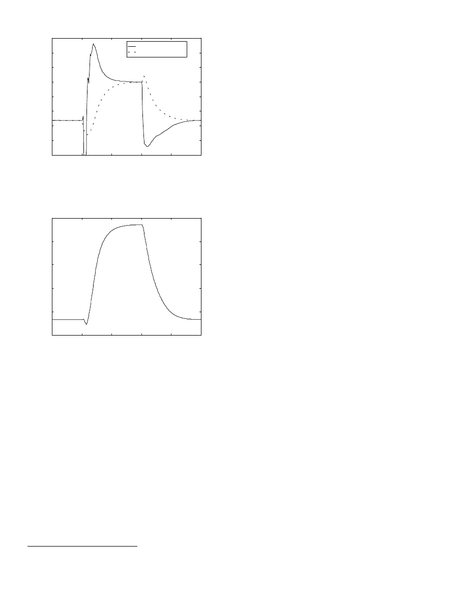
0.5

1

1.5

2

2.5

3

0

10

20

30

40

50

In

ta

k

e

P

o

rt

A

/F

Time (sec)

Figure 21: Intake port air/fuel ratio using a speed-density fuel

calculation

The larger lean air/fuel excursion for the speed-density

baseline causes a significant drop in indicated torque after the
throttle tip-in (as shown in Fig. 22). The longer duration drop
in torque is caused by more cylinders misfiring due to the lean
condition (as compared to the air mass sensor baseline),
causing a noticeable drop in engine speed (see Fig. 23). The
drop in speed would probably be felt as a “stumble” if the
engine were running in a vehicle.

SAE 950417

Weeks & Moskwa 3/24/95

-9-

Indicated

Friction/Pumping

0.5

1

1.5

2

2.5

3

0

20

40

60

80

100

120

140

160

Tor

q

u

e

(

N

*m

)

Time (sec)

Figure 22: Engine indicated and friction/pumping torque using

a speed-density fuel calculation

0.5

1

1.5

2

2.5

3

200

300

400

500

600

700

En

g

in

e

Speed

(

rad/

s)

Time (sec)

Figure 23: Engine speed using a speed-density fuel

calculation (note tip-in “stumble”)

Fuel Dynamics Parametric Study

One of the advantages of using S

IMULINK

is that models

can be developed and run interactively using a graphical
interface and also run from the M

ATLAB

command line. This

makes it easier to perform parametric analyses to examine the
effects of varying different constants in the model. With the
help of optimization tools the model parameters can often be
automatically “tuned” to minimize a “cost” function and thus
maximize some user-defined performance criteria. It is
sometimes possible to “fit” the model to measured engine data
by using commercially available optimization algorithms to
automatically adjust model parameters.

*

This subsection demonstrates how the engine model may

be used in a simple fuel dynamics parametric study to
determine the effects of varying some of the fuel parameters
mentioned earlier. The first parameter varied is the start of
injection to intake valve closing angle (SOItoIVC_deg).

*

The Levenberg-Marquardt method was originally used

to identify the dynamic fuel parameters for this model from
engine data on a dynamometer [3].

SOItoIVC_deg represents the number of degrees the
crankshaft rotates from when the fuel injector is opened to
when the intake valve (for that injector’s cylinder) closes.
Most sequential port fuel injection systems control the timing
of the injection relative to the intake valve opening so there is
an interest in understanding how this affects air/fuel ratio
control and emissions.

There is a transient fueling advantage for waiting until the

intake valve nearly closes before injecting a given cylinder’s
fuel, but if the injector is still open after the valve closes, part
of the fuel will have to wait in the intake port for nearly two
revolutions until the valve opens again. This contributes to
transient air/fuel ratio errors.

There is often a steady-state fueling advantage to injecting

fuel after the intake valve closes so it has the longest possible
residence time in the intake port. This allows more time for
the fuel to vaporize in the vicinity of a hot intake valve and can
sometimes lower steady-state emission levels.

The two strategies are diametrically opposed to one

another making it difficult to determine the best time to inject
fuel relative to the intake valve closing. The engine and
control system model can be used to help evaluate fueling
strategies related to transient air/fuel control and how it is
affected by injection timing. The following M

ATLAB

script

file shows how the engine and control system model shown in
Fig. 1 can be executed within a loop to determine the effect of
varying SOItoIVC_deg:

clear

% clear the workspace before starting

% define some global variables

global SOItoIVC_deg aferror x0 options

% load vehicle specific data into workspace

simspec

load initcond; % get initial conditions for states

% set fuel calculation flag

UseAMS=0; % 1=air-mass sensor, 0=speed-density

options=[1e-8,0.0001,0.001]; % set simulation options

for i=0:3

% initialize fuel injection parameter

SOItoIVC_deg=240*i;

% create a filename to store simulation results

filename=['SOI',int2str(i),'.mat'];

% simulate the engine and control system model

[t,x,yo]=rk45('engsim',[0.0,3.0],x0,options);

% save the results for later analysis

eval(['save ',filename,' y aferror']);

end

The above script file performs four separate simulations

of the engine and control system model (engsim.m) using a
Runge-Kutta integration algorithm. SOItoIVC_deg is varied
from 0 degrees up to 720 degrees in 240 degree increments.
The results of each simulation are stored in a different file as
follows:

SAE 950417

Weeks & Moskwa 3/24/95

-10-

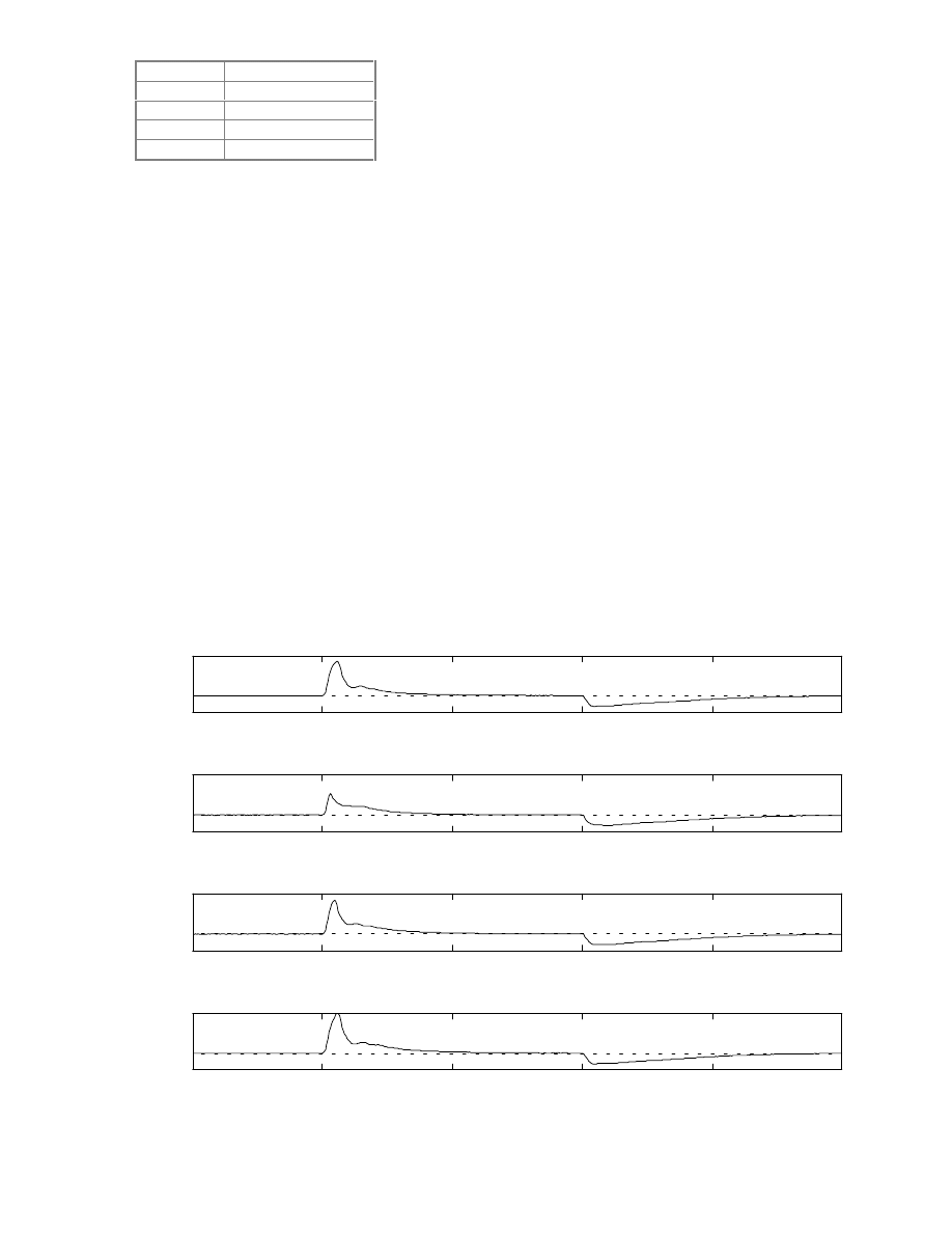
Another m-file was written to load the results and plot the

intake port air/fuel ratio versus simulation time (shown in Fig.
24). In the first run the fuel is injected right as the intake valve
closes where it would remain in the port for nearly two
revolutions before the valve reopens. During the throttle
transient the air flow rate changes significantly during two
revolutions of the crankshaft. This effect contributes a
substantial portion of the air/fuel ratio error shown in the first
run. In the second run (where SOItoIVC_deg=240) the fuel
injection is completed at about the same time as the intake
valve closing. This helps to minimize the transient air/fuel
errors but does not allow the fuel as much time to vaporize in
the intake port. The third and fourth runs show that when fuel
is injected a significant time before the intake valve closes the
transient air/fuel errors will again increase. To help minimize
these transient air/fuel ratio errors, some injection strategies
control the end of injection relative to intake valve closure
rather than the start of injection.

Previous steady state engine testing has shown that

injection of fuel while the intake valve is open can lead to
increased emissions (due to poor vaporization and exhaust
backflow effects) but injection of fuel while the valve is closed
can lead to transient air/fuel ratio errors (which also leads to
increased emissions). An ideal strategy would be one that

could predict the air flow rate at the ports approximately two
crankshaft revolutions in the future and then inject the proper
fuel pulse (allowing for fuel dynamics) right after the intake
valve closes. This would allow the most time for fuel
vaporization but would not suffer from transient air/fuel errors
due to injection timing. An accurate prediction of future port
air flow rates would require a drive-by-wire throttle so the
engine controller could know the throttle’s trajectory over the
next two crankshaft revolutions. Then using an embedded
intake manifold model (similar to the one described in this
paper), the controller would predict future port air flow rates
as part of its fuel calculation. This is one of the authors’
current research topics and is more thoroughly described in
[4].

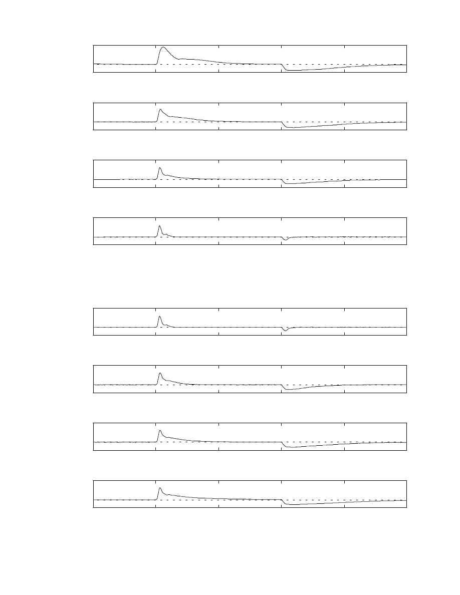
Fig. 24 illustrates a set of parametric runs showing the

effects of varying SOItoIVC_deg. A similar set of parametric
runs were performed where the values used for the fuel split
parameter (epsilon) and the slow fuel time constant (tauf) were
varied. These results are shown in Figs. 25 and 26. As epsilon
approaches a value of one (see fourth plot in Fig. 25) the liquid
fuel dynamics become negligible and most of the air/fuel error
is due to the pure time delay,

∆

T

1

(see subsection on fuel

dynamics). A similar effect occurs as the slow fuel time
constant (tauf) approaches zero (shown in the first plot in Fig.
26).

The example simulations and the parametric study

presented here illustrate some of the possible uses of the mean
torque predictive engine model. Other uses of the model are
described (but not illustrated) in the SUMMARY and
CONCLUSIONS section.

0.5

1

1.5

2

2.5

3

0

50

A/

F r

a

ti

o

SO ItoIVC_deg= 0

0.5

1

1.5

2

2.5

3

0

50

A/

F r

a

ti

o

SO ItoIVC_deg= 240

0.5

1

1.5

2

2.5

3

0

50

A/

F r

a

ti

o

SO ItoIVC_deg= 480

0.5

1

1.5

2

2.5

3

0

50

A/

F r

a

ti

o

SO ItoIVC_deg= 720

Time (sec)

Figure 24: Effects of varying start of injection relative to intake valve closing

file name

test condition

SOI0.mat

SOItoIVC_deg=0

SOI1.mat

SOItoIVC_deg=240

SOI2.mat

SOItoIVC_deg=480

SOI3.mat

SOItoIVC_deg=720

SAE 950417

Weeks & Moskwa 3/24/95

-11-

0.5

1

1.5

2

2.5

3

0

50

A/

F r

a

ti

o

epsilon= 0.00

0.5

1

1.5

2

2.5

3

0

50

A/

F r

a

ti

o

epsilon= 0.33

0.5

1

1.5

2

2.5

3

0

50

A/

F r

a

ti

o

epsilon= 0.66

0.5

1

1.5

2

2.5

3

0

50

A/

F r

a

ti

o

epsilon= 1.00

Time (sec)

Figure 25: Effects of varying fuel split parameter, epsilon

0.5

1

1.5

2

2.5

3

0

50

A/

F r

a

ti

o

tauf= 0.001

0.5

1

1.5

2

2.5

3

0

50

A/

F r

a

ti

o

tauf= 0.11

0.5

1

1.5

2

2.5

3

0

50

A/

F r

a

ti

o

tauf= 0.22

0.5

1

1.5

2

2.5

3

0

50

A/

F r

a

ti

o

tauf= 0.33

Time (sec)

Figure 26: Effects of varying slow fuel time constant, tauf

SAE 950417

Weeks & Moskwa 3/24/95

-12-

SUMMARY and CONCLUSIONS

An automotive engine model designed for real-time

control applications has been presented in the context of a
S

IMULINK

engine and control system model. Subsystems

within the model were briefly described with some additional
detail related to the air and fuel dynamics portion of the intake
manifold subsystem. Example simulations were presented to
show some of the potential uses of the model.

In general, the model may be used in five different ways:

1. As a nonreal-time engine model for testing engine

control algorithms. Nonreal-time testing allows
researchers and engineers to develop new control
algorithms without the hardware constraints and
software complexities of running in real-time.

*

This

allows new ideas to be rapidly evaluated using high
level languages such as graphical block diagrams or C.
High precision floating point calculations can be used
on low cost computers to rapidly iterate algorithm
designs until a robust control law is found. Algorithms
can often be evaluated in a matter of minutes or hours,
whereas many conventional development systems
require days or weeks to test new ideas because control
algorithms must be written in assembler and tested on
an actual vehicle.

2. As a real-time engine model for hardware-in-the-

loop testing. Many engine models do a good job of
simulating the dynamic behavior of an engine but are
not designed to run in real-time. The engine model
presented here, is physically based but relatively simple
and uses a large number of table look-ups to reduce
execution time. When converted to C (see appendix),
the model may be executed on a variety of target
processors. With a relatively low cost processor and
appropriate I/O, the model may be used to evaluate the
performance of actual engine sensors, controllers or
actuators. For example, an actual engine controller
(ECU) could be tested in a highly repeatable and
deterministic manner using off-the-shelf simulation
hardware [7].

3. As an embedded model within a control algorithm

or observer. As model-based controls become more
popular, simplified versions or subsystems of an engine
model are often embedded into a real-time control
algorithm [4-6,8-19]. The embedded model can predict
engine variables that are difficult or impractical to
measure. Observers or state estimators can also be used
for diagnostic purposes, such as those mandated by
OBDII.

4. As a system model for evaluating engine sensor and

actuator models. Vehicle manufacturers will eventually
require suppliers to provide models of the components

*

Some examples of nonlinear sliding mode engine control

algorithms (tested on the original FORTRAN version of the
engine model described in this paper) are given in [5,6]. The
algorithms use coordinated throttle and spark advance control
to force the engine to track desired engine and transmission
speed trajectories.

they sell so the manufacturer can do system simulations
before prototype vehicles are built. When used as a
system model, the engine and control system model can
evaluate different sensor and actuator models. The
modular design allows new sensor and/or actuator
models to be tested without modifying the engine
model. This makes it easier for component suppliers to
perform system simulations of their sensor or actuator
models without having to develop their own engine
models.

5. As a subsystem in a powertrain or vehicle dynamics

model. Mean torque predictive engine models are often
incorporated into larger powertrain or vehicle dynamics
models [20-23]. In general, as the complexity and size
of a system model increases, the complexity of
subsystem models must be reduced. Because of their
relatively simple nature, mean torque predictive engine
models are often more appropriate for vehicle
simulations than models that predict individual cylinder
filling phenomena.

Simulations are used by a large number of control system

researchers but there is very little standardization in the plant
models used for developing control laws. This makes it
difficult to evaluate research showing the benefits of different
control theories. A validated benchmark model makes it easier
for control engineers at the vehicle manufacturers to evaluate
control algorithms developed by researchers at various
academic institutions. A benchmark model will allow
comparison of new control algorithms in a very direct and
repeatable manner. This will make it easier for vehicle
manufacturers to identify promising control theories and
techniques.

REFERENCES

[1]

Moskwa, J.J., “Automotive Engine Modeling for Real-
time Control,” Department of Mechanical Engineering,
M.I.T., Ph.D. thesis, 1988.

[2]

Moskwa, J.J. and Hedrick, J.K., “Modeling and
Validation of Automotive Engines for Control
Algorithm Development,” ASME J. of Dynamic
Systems, Measurement and Control, Vol. 114, No. 2,
pp. 278-285, June 1992.

[3]

Moskwa, J.J., “Estimation of Dynamic Fuel Parameters
in Automotive Engines,” ASME J. of Dynamic Systems,
Measurement and Control, December 1994.

[4]

Weeks, R.W. and Moskwa, J.J., “Transient Air Flow
Rate Estimation in a Natural Gas Engine Using a
Nonlinear Observer,” SAE paper No. 940759, 1994.

[5]

Moskwa, J.J., “Sliding Mode Control of Automotive
Engines,” ASME J. of Dynamic Systems, Measurement
and Control, Vol. 115, No. 4, pp. 687-693, December
1993.

SAE 950417

Weeks & Moskwa 3/24/95

-13-

[6]

Moskwa, J.J. and Hedrick, J.K., “Nonlinear Algorithms
for Automotive Engine Control,” IEEE Control Systems
Magazine, Vol. 10, No. 3, pp. 88-93, April 1990.

[7]

Hanselmann, H., “DSP-Based Automotive Sensor
Signal Generation for Hardware-in-the-Loop
Simulation,” SAE paper No. 940185, 1994.

[8]

Hendricks, E., Vesterholm, T. and Sorenson, S. C.,
“Nonlinear, Closed-loop, SI Engine Control
Observers,” SAE paper No. 920237, 1992.

[9]

Kaidantzis, P., et al., “Advanced Nonlinear Observer
Control of SI Engines,” SAE paper 930768, 1993.

[10]

Chang, C., Fekete, N.P. and Powell, J.D., “Engine Air-
Fuel Ratio Control Using an Event-Based Observer,”
SAE paper 930766, 1993.

[11]

Kao, M.H. and Moskwa, J.J., “Engine Load and
Equivalence Ratio Estimation for Control and
Diagnostics via Nonlinear Sliding Observers,”
International Journal of Vehicle Design, Vol. 15, No.
3/4, 1994..

[12]

Shiao, Y.J. and Moskwa, J.J., “Cylinder Pressure and
Combustion Heat Release Estimation for SI Engine
Diagnostics Using Nonlinear Sliding Observers,” IEEE
Transactions on Control Systems Technology, March
1995.

[13]

Kao, M.H. and Moskwa, J.J., “Nonlinear Diesel Engine
Control and Cylinder Pressure Observation,” ASME J.
of Dynamic Systems, Measurement and Control ,
(accepted March 1994).

[14]

Shiao, Y. and Moskwa, J.J., “Misfire Detection and
Cylinder Pressure Reconstruction for SI Engines,” SAE
paper No. 940144

*

, 1994.

[15]

Ault, B.A., et al., “Adaptive Air-Fuel Ratio Control of a
Spark-Ignition Engine,” SAE paper No. 940373, 1994.

[16]

Turin, R.C. and Geering, H.P., “Model-Based Adaptive
Fuel Control in an SI Engine,” SAE paper No. 940374,
1994.

[17]

Kao, M.H. and Moskwa, J.J., “Nonlinear Cylinder and
Intake Manifold Pressure Observers for Engine Control
and Diagnostics,” SAE paper No. 940375, 1994.

[18]

Amstutz, A., et al., “Model-Based Air-Fuel Ratio
Control in SI Engines with a Switch-Type EGO
Sensor,” SAE paper No. 940972, 1994.

[19]

Cho, D. and Oh, H., “Variable Structure Control
Method for Fuel-Injected Systems,” ASME J. of

*

References [14-17] can also be found in SAE special

publication Electronic Engine Controls 1994 (SP-1029).

Dynamic Systems, Measurement and Control, Vol. 115
Sept. 1993.

[20]

Cho, D., “Nonlinear Control Methods for Automotive
Powertrain Systems,” Department of Mechanical
Engineering, M.I.T., Ph.D. thesis, 1987.

[21]

Cho, D. and Hedrick, J.K., “Automotive Powertrain
Modeling for Control,” ASME J. of Dynamic Systems,
Measurement and Control, 114(4), pp. 568-576, 1989.

[22]

Weeks, R.W., “Implementation Issues in Sliding Mode
Automotive Powertrain Controllers,” Department of
Mechanical Engineering, M.I.T., Sc.M. thesis, 1988.

[23]

McMahon, D.H., et al., “Longitudinal Vehicle
Controllers for IVHS: Theory and Experiment,” in
Proc. American Contr. Conf., 1992.

[24]

The MathWorks, Inc., S

IMULINK

Accelerator User's

Guide, April, 1994.

[25]

The MathWorks, Inc., S

IMULINK

Real-Time Workshop

User's Guide, May, 1994.

NOMENCLATURE

ADC

analog to digital converter

alpha

throttle angle (degrees)

AMS

air-mass sensor

AMStau

air-mass sensor time constant (s)

C

1

speed-density constant

DSP

digital signal processor

EGR

exhaust gas recirculation

EngSpeed,

ω

e

engine speed (rad s)

epsilon,

ε

fuel split parameter

gamma,

γ

fraction of fuel injected before IVC

IAC

idle air control

IVC

intake valve close

MBT

minimum spark for best torque (DBTDC)

.m, m-file

M

ATLAB

ASCII file

.mex, MEX-file M

ATLAB

object code file

mdot_ai, m

ai

•

air flow rate into intake ( kg s )

mdot_ao, m

ao

•

air flow rate into cylinder (kg s )

mdot_egri,

m

egri

•

EGR flow rate into intake (kg s )

mdot_egro,

m

egro

•

EGR flow rate into cylinder (kg s )

mdot_fi,

m

fi

•

fuel flow rate at injector ( kg s )

mdot_fo,

m

fo

•

fuel flow rate into cylinder ( kg s )

mdot_ff2,

m

ff

•

2

fuel flow injected after IVC ( kg s )

mdot_ff3,

m

ff

•

3

fuel flow injected before IVC ( kg s )

mdot_fs1,

m

fs

•

1

fuel flow lagged by wall wetting ( kg s )

OBDII

On-Board Diagnostics II

Pamb

ambient air pressure (kPa)

Pexh

exhaust manifold pressure (kPa)

Pman

intake manifold pressure (kPa)

SAE 950417

Weeks & Moskwa 3/24/95

-14-

R

perfect gas constant (for air R=

287 J kg K

°

)

S/D

speed-density

SFI

sequential fuel injection

SOI

start of injection

SOItoIVC_deg

Φ

Φ

IVC

SOI

−

VE,

η

vol

volumetric efficiency of engine (unitless)

Veng,

V

disp

engine displacement (

m

3

)

Vman

intake manifold volume (

m

3

)

tauf,

τ

f

slow fuel time constant (s)

Tamb

ambient air temperature (

°

K

)

Tman

intake manifold temperature (

°

K

)

Φ

SOI

crank angle at start of injection (degrees)

Φ

IVC

crank angle at intake valve close (degrees)

Φ

PW

injector pulse width in crank degrees

∆

T

1

, delta t1

fuel time delay from command to IVC (s)

∆

T

2

, delta t2

two crank revolution fuel time delay (s)

S

IMULINK

™ block diagram symbol

APPENDIX

S

IMULINK

Benchmarks

This section presents some of the execution times for the

engine and control system models described earlier in the
paper so readers can gauge the approximate time the models
would take to run on their platform. The models described in
this paper were all simulated on a 50Mhz PC with 16Mb of
RAM using M

ATLAB

4.2 and S

IMULINK

1.3. Some of the

simulations described later in the appendix also required the
use of two additional MathWorks “toolboxes.” For these
simulations, the S

IMULINK

Accelerator™ (version 1.1) and

the Real-Time Workshop™ (version 1.1a) were used. The
Accelerator and the Real-Time Workshop both require a C
compiler. For this, a WATCOM C/C++ 32 bit compiler was
used (version 9.5b).

The standard M

ATLAB

benchmark program (bench.m)

was run on the PC used to perform the S

IMULINK

simulations.

Its performance relative to a group of other computers is
shown in Fig. A1 so readers can assess how their platform
compares to the PC used to run the engine and control system
models. The PC’s performance is shown as “This computer”
in the bar chart in Fig. A1. The bar chart shows relative speed,
which is inversely proportional to the execution time. Longer
bars are faster machines, shorter bars are slower.

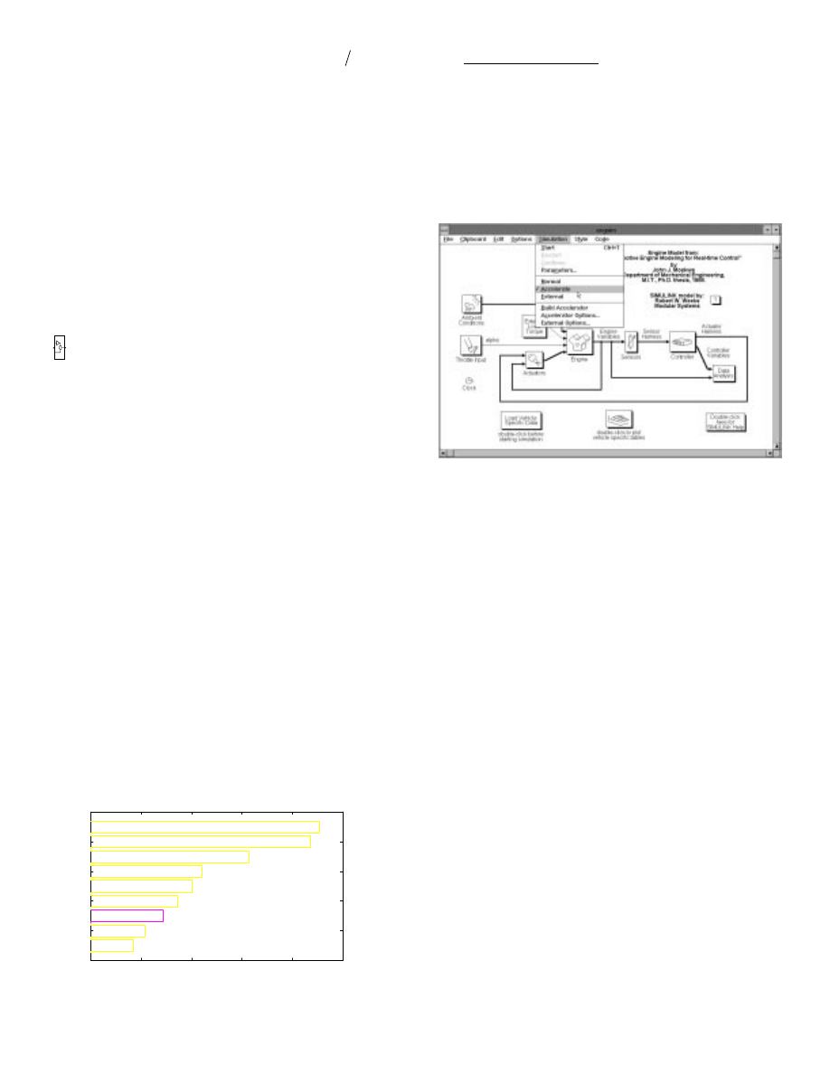
0

50

100

150

200

250

0

2

4

6

8

10

Relative Speed

SPARC-1

Tadpole

This computer

IBM RS/6000, 320

SPARC-2

Iris Indigo

HP 710

SPARC-10

HP 720

Figure A1: PC’s performance (“This computer”) relative to

several other computers executing the M

ATLAB

benchmark

S

IMULINK

Accelerator

The S

IMULINK

Accelerator increases the speed of a

simulation by generating C code for the S

IMULINK

model,

compiling it as a M

ATLAB

MEX-file, and dynamically linking

it in place of the original internal model representation. When
the Accelerator is enabled (as shown in Fig. A2) and a
simulation is started, S

IMULINK

first looks for a MEX-file

whose name matches that of the S

IMULINK

model. If the

MEX-file does not exist or is not up to date a new MEX-file is
automatically generated and executed.

Figure A2: Enabling the simulation “Accelerate” option

Some of the simulations in the Fuel Dynamics

Parametric Study (presented earlier) were run both with and
without the “Accelerate” option enabled. Without the
accelerator a set of four simulations took 548.8 seconds to
execute on a 50Mhz 486 PC. With the accelerator enabled the
simulation time dropped to 148.8 seconds for an improvement
factor of 3.7. As the complexity and number of blocks in a
model increases the improvement factor also tends to increase
to an upper limit of about 7.1 [24].

When running short simulations during model

development it is sometimes better to disable the accelerate
option if a lot of changes are being made to the block diagram.
This avoids the time taken to generate and compile the C code
before a “run” is made. If the simulations take longer than a
minute or so, it is usually faster to use the Accelerator even if
it has to regenerate and recompile the C code before each run.
For example, the engine and control system model takes 135
seconds to run one “3 second” simulation when the
Accelerator is not present, dropping to 40 seconds (for an
improvement factor of 3.37) if the Accelerator is enabled but it
does not have to regenerate or recompile C code.

If a change is made to the block diagram that forces the

Accelerator to regenerate C code, the total simulation time
increases to about 88 seconds of which 54 seconds are
required to generate and compile the C code and 34 seconds
are required to run the simulation. For most reasonably large
models it is best to always leave the Accelerator enabled.

The C code generated by the Accelerator option is

uncommented and cannot be compiled and run as a standalone
program. The S

IMULINK

Real-Time Workshop should be

used if commented C source code is desired that can be
compiled and run on a variety of target processors.

SAE 950417

Weeks & Moskwa 3/24/95

-15-

S

IMULINK

Real-Time Workshop

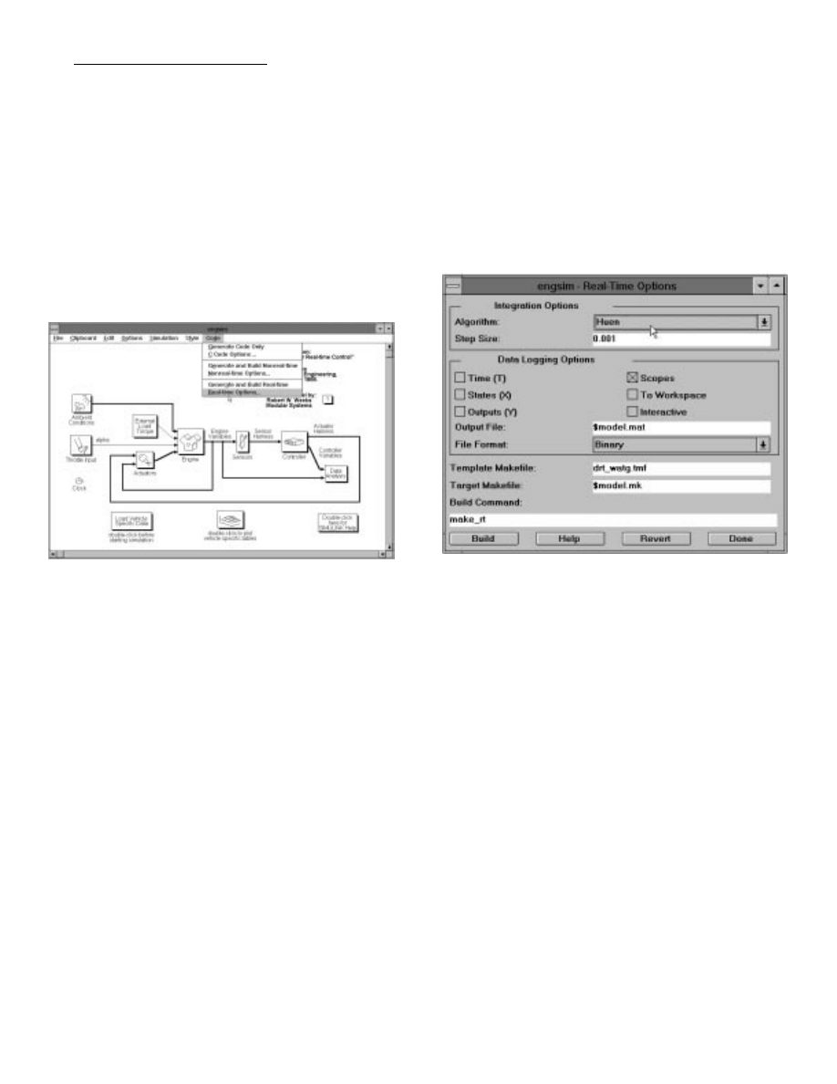
The S

IMULINK

Real-Time Workshop is an automatic C

language generation environment for S

IMULINK

. It produces

C code directly from S

IMULINK

graphical models and

automatically builds programs that can be run in real-time in a
variety of environments [25]. With the Workshop, S

IMULINK

models can be run in real-time on a remote processor
(assuming the processor is sufficiently fast). It can also be
used to generate accelerated stand-alone versions of models
that can be run on the host computer or on an external
computer. C source code can be generated for both real-time
and nonreal-time simulations. When “Real-time Options...” is
selected with the mouse (as shown in Fig. A3) a dialog box
(shown in Fig. A4) appears to allow some customization of
options such as the integration algorithm and step size and data
logging.

Figure A3: Selecting the C code generation real-time options

The engine and control system model shown in Fig. A3

will not run in real-time on a 50Mhz PC. A nonreal-time DOS
executable model (generated using the “Nonreal-time
Options”) will perform a “3 second” simulation run in 25
seconds of actual time using variable time step Runge-Kutta
integration. Running the same model using Euler integration
and a fixed time step of 1/2 millisecond reduces the simulation
time to 9 seconds but with a slight loss in simulation accuracy.
Real-time execution speeds should be possible on a PC based
DSP board or possibly on a higher clock speed Pentium PC.
The authors plan to determine the minimum platform needed
for real-time execution so that hardware-in-the-loop testing can
be performed using the engine model in place of a real engine.

Figure A4: Options available for real-time code generation

(after selecting “Real-time Options...” in Fig A3)