k-Convex Polygons

∗

O. Aichholzer

†

F. Aurenhammer

‡

E. D. Demaine

F. Hurtado

P. Ramos

J. Urrutia

∗∗

July 22, 2010

Abstract

We introduce a notion of k-convexity and explore polygons in the plane that

have this property. Polygons which are k-convex can be triangulated with fast yet
simple algorithms. However, recognizing them in general is a 3SUM-hard problem.
We give a characterization of 2-convex polygons, a particularly interesting class,
and show how to recognize them in O(n log n) time. A description of their shape is
given as well, which leads to Erd˝os-Szekeres type results regarding subconfigurations
of their vertex sets. Finally, we introduce the concept of generalized geometric
permutations, and show that their number can be exponential in the number of
2-convex objects considered.

Introduction

The notion of convexity is central in geometry. As such, it has been generalized in
many ways and for different reasons. In this paper we consider a simple and intuitive
generalization of convexity, which to the best of our knowledge has not been worked on.
It leads to an appealing class of polygons in the plane with interesting structural and
algorithmic properties.

A set in R

is convex if its intersection with every straight line is connected. This

definition may be relaxed to directional convexity or D-convexity [15, 23], by considering
only lines parallel to one out of a (possibly infinite) set D of vectors. A special case is

∗

Partially supported by the FWF Joint Research Program ‘Industrial Geometry’ S9205-N12, Projects

MEC MTM2006-01267, DURSI 2005SGR00692, Project Gen. Cat. DGR 2009SGR1040, DGR 2009SGR-
1040, MEC MTM2009-07242, MEC MTM2008-04699-C03-02, and the bilateral Spain-Austria program
‘Acciones Integradas’ ES 01/2008 and HU2007-0017.

†

Institute for Software Technology, University of Technology, Graz, Austria, oaich@ist.tugraz.at

‡

Institute

for Theoretical Computer Science,

University of Technology,

Graz,

Austria,

auren@igi.tugraz.at

Computer Science and Artificial Intelligence Laboratory, Massachusetts Institute of Technology,

Cambridge, USA, edemaine@mit.edu

Departament de Matem`

atica Aplicada II, Universitat Polit`ecnica de Catalunya, Barcelona, Spain,

Ferran.Hurtado@upc.edu

Departamento de Matem´

aticas, Universidad de Alcal´

a, Madrid, Spain, pedro.ramos@uah.es

∗∗

Instituto de Matem´

aticas, Universidad Nacional Aut`

onoma de M`exico, urrutia@matem.unam.mx

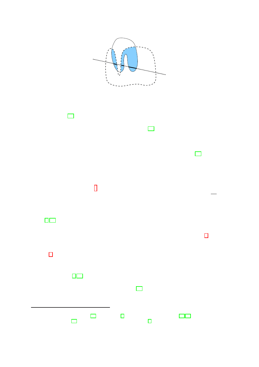
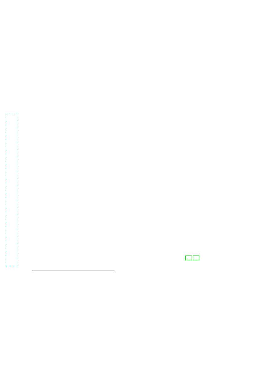
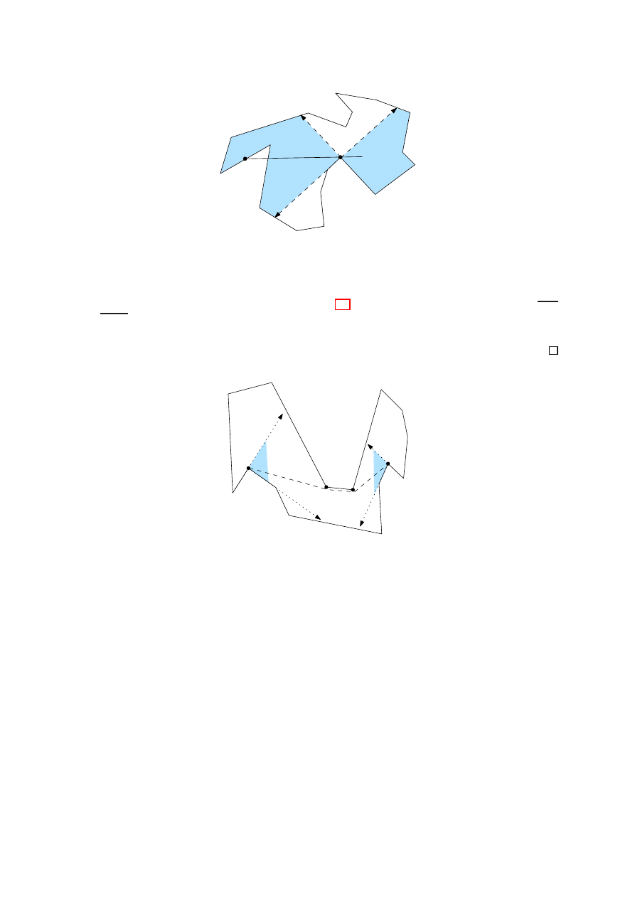
Figure 1: Intersecting two 2-convex sets

ortho-convexity [27], where only horizontal and vertical lines are allowed. For any fixed D,
the family of D-convex sets is closed under intersection, and thus can be treated in a sys-
tematic way using the notion of semi-convex spaces [29], which is sometimes appropriate
for investigating visibility issues. The D-convex hull of a set M is the intersection of
all D-convex sets that contain M. If D is a finite set, this definition of a convex hull
may lead to an undesirably sparse structure—an effect which can be remedied by using
a stronger, functional (rather than set-theoretic) concept of D-convexity [23].

-Convex Sets

We consider a different generalization of convexity. A set M in R

is called k-convex (with respect to transversal lines) if there exists no straight line that
intersects M in more than k connected components. Throughout the paper we will use
the term k-convex , for short

. Note that 1-convexity refers to convexity in its standard

meaning. To reformulate in terms of visibility, call two points x, y

∈ M k-visible if xy ∩ M

consists of at most k components. Thus a set is k-convex if and only if any two of its
points are mutually k-visible. Applications of this concept may arise from placement
problems for modems that have the capacity of transmitting through a fixed number of
walls [1, 13].

Unlike directional convexity, k-convexity fails to show the intersection property: The

intersection of k-convex sets is not k-convex in general (for fixed k). Figure 1 gives an
example. For k

≥ 2, a k-convex set M may be disconnected, or if connected, its boundary

may be disconnected. In this paper, we will restrict attention (with an exception in
Section 4) to simply connected sets in two dimensions, namely, simple polygons in the
plane.

There are two notions of planar convexity that appear to be close to ours. One is

k-point convexity [6,32] which requires that for any k points in a set M in R

, at least one

of the line segments they span is contained in M. Thus 2-point convex sets are precisely
the convex sets. The other is k-link convexity [22], being fulfilled for a given polygon P
if, for any two points in P , the geodesic path connecting them inside P consists of at
most k edges. The 1-link convex polygons are just the convex polygons. While there is a

We face notational ambiguity. The term ‘k-convex’ has, maybe not surprisingly, been used in different

settings, namely, for functions [26], for graphs [5], and for discrete point sets [20, 33]. Also, the concept
of k-point convexity [32] has later been called k-convexity in [6].

relation between k-convexity and the former concept (as we will show in Section 2), the
latter concept is totally unrelated.

We will study basic properties of k-convex polygons, in comparison to existing polygon

classes and convexity concepts in Section 2. This offers an alternative to the approach
in [4] to define ‘realistic’ polygons as those being guardable (visible) by at most k guards.
We prove that given a simple polygon P , the problem of finding the smallest k such that
P is k-convex (equivalently, to find the stabbing number of P ) is 3SUM-hard. On the
other hand, a recognition algorithm that runs in O(n

) time for a polygon with n vertices

is easy to obtain. Interestingly, k-convex polygons can be triangulated, by a quite simple
method, in O(n log k) time. An O(nk) time complexity is achieved in [4] for k-guardable
polygons.

The first nontrivial value, k = 2, deserves particular attention. Already in this case,

a novel class of polygons is obtained. A characterization of 2-convex polygons is given in
Section 3. It leads to an O(n log n) time algorithm for recognizing such polygons. Note
that 2-convex polygons add to the list of special classes of polygons [4, 11] that allow
for simple O(n) time triangulation methods. We also provide a qualitative description
of their shape, which implies an Erd˝os-Szekeres type result, namely, that every 2-convex
polygon with n vertices contains a subset of at least

√

n vertices in convex position, and

that its vertex set can be decomposed into at most 2

√

2n subsets in convex position.

In Section 4, we turn our attention to general k-convex domains. We give observations

on the union and intersection properties of such domains, and elaborate on an attempt
to generalize the notion of geometric permutations from convex sets to k-convex sets.
In contrast to the O(m) bound in [10] on the number of geometric permutations of m
convex sets, it turns out that the number of generalized geometric permutations can be
exponential in m, already for 2-convex sets. For 2-convex polygonal domains, the number
of generalized geometric permutations is O(n

), if n denotes the total number of their

vertices.

Various open questions are raised by the proposed concept of k-convexity. We list

those which seem most interesting to us, along with a brief discussion of our results, in
Section 5.

k-Convex Polygons

2.1

Basic properties

We start with exploring some basic properties of k-convex polygons, and compare them
to existing polygon classes and related concepts. All geometric objects we will consider
are closed sets in the Euclidean plane.

Let P be a simple polygon, and denote by n the number of vertices of P . Two line

segments e and e

′

are said to cross if e

∩ e

′

is a point in the relative interior of both e

and e

′

. Clearly, a polygon P is k-convex if every line segment with endpoints in P crosses

at most 2(k

− 1) edges of P . The stabbing number [14, 35] of a set of (interior-disjoint)

line segments is the largest possible number of intersections between the set and a straight
line. A polygon is k-convex if and only if its stabbing number is at most 2k. Thus, all

our observations on k-convexity could be reformulated in terms of stabbing numbers.
Moreover, we have the following property, which we state for future reference.

Lemma 1.

If P is a k-convex polygon, then any polygon living on a subset of vertices of

P is also k-convex.

(a)

(b)

Figure 2: Quadratic 2-kernel construction

The kernel of a simple polygon P is the set of points that see all the polygon. Its

generalization to k-convexity shows that 2-convexity is already significantly more complex
than standard convexity. The k-kernel of P , denoted as M

(P ), is the set of points from

which the entire polygon P is k-visible. Note that P is k-convex if and only if P = M

While M

is known to be a convex set which is computable in O(n) time [21], M

may

have Ω(n

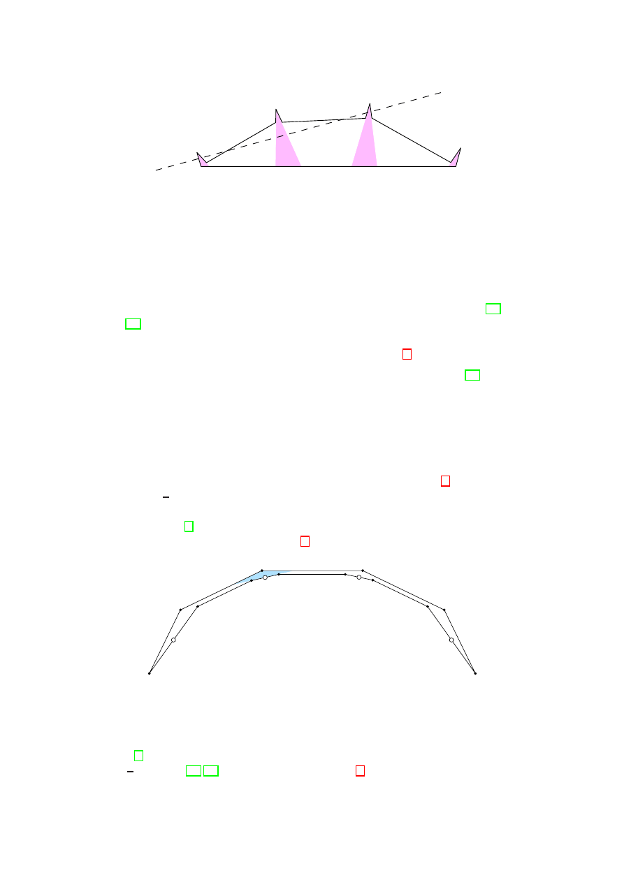
) complexity: If we consider the ‘spike’ in Figure 2(a), the wedge between

the lines pq and pr is not part of M

. If we arrange such spikes along the boundary of

a rectangle, as in Figure 2(b), we get a quadratic number of disconnected areas which
are part of the 2-kernel. Therefore, any algorithm computing M

, or trying to check

2-convexity via the comparison of P and M

would have Ω(n

) complexity in the worst

case.

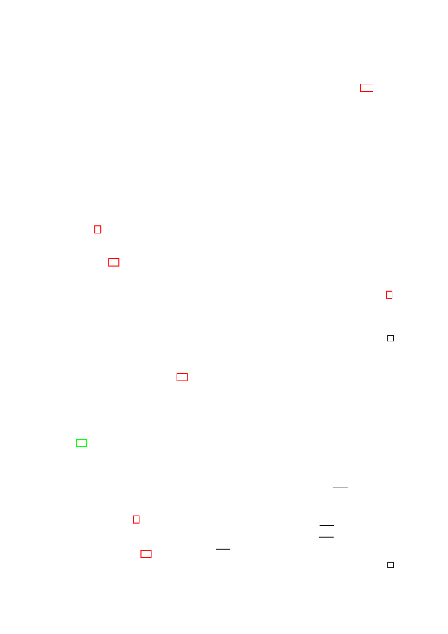
Figure 3: Star-shaped versus 2-convex

There is also no immediate relation to star-shaped polygons, i.e., polygons P with M

∅. Figure 3 shows a polygon on the left hand side which is star-shaped but only

-convex.

Figure 4: Guarding a 3-convex polygon

On the right hand side, we see a polygon which is 2-convex but not star-shaped. Visually,
2-convexity seems to be closer to convexity than is star-shapedness. Note that cutting a
2-convex polygon with any straight line leaves (at most) three parts, each being 2-convex
itself. This is not true in general for star-shaped polygons.

While 2-convexity obviously restricts the winding number of a polygon [34], its link

distance [22] is unaffected and may well be Θ(n). Conversely, a polygon which is 2-link
convex (such that any two of its points are at link distance 2 or less) may fail to be
k-convex for sublinear k. The star-shaped polygon in Figure 3 (left) is an example.

There is, interestingly, a relation to k-point convexity as defined in [32]. A polygon

P is called k-point convex if for any k points p

, . . . , p

in P , at least one of the closed

segments p

belongs to P . Every k-point convex polygon P is (k

− 1)-convex. To verify

this, we prove that if P is not (k

− 1)-convex, then P is not k-point convex: Because P

is not (k

− 1)-convex, there exists a line ℓ which intersects P in at least k components.

If we select a point in each component, it is clear that none of the segments defined by
them is inside P , and therefore P is not k-point convex. However, no implication exists
in the other direction. For example, the 2-convex polygon in Figure 5 fails to be k-point
convex for k <

. Also, any k-point convex polygon can be expressed as the union of

m convex polygons, where m depends (exponentially) on k but is independent of the
polygon size n; see [6]. Such a property is not shared by k-convex polygons, as can be
seen from the 2-convex polygon in Figure 5.

Figure 5: Every white dot requires a different guard

The class of k-convex polygons also differs from the class of k-guardable polygons

defined in [4]. It is known that any simple polygon with n vertices can be guarded with
at most

⌊

⌋ guards [25, 31]. The example in Figure 5 shows that this number of guards

can be already necessary for 2-convex polygons. This is one of the reasons why most

tools developed to study guarding problems of polygons are not very useful in the study
of modem illumination problems [1].

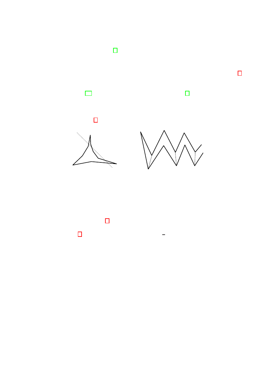
Pseudo-triangles are polygons with exactly three convex vertices, joined by three

reflex side chains. Any pseudo-triangle is 2-convex: If a straight line crosses a side chain
twice, then it can cross each of the remaining two side chains at most once (Figure 6,
left). That is, the stabbing number of a pseudo-triangle is four or less. In the same way
as a triangulation defines a partition of the underlying domain into convex polygons, any
pseudo-triangulation [28] or any pseudo-convex decomposition [3] gives a partition into
2-convex polygons. It is an open problem (see Problem(e) in the final section) whether
it is possible to subdivide a polygon with n vertices into a sublinear number of 2-convex
polygons. If Steiner points are disallowed, then a 2-convex partition may have to consist
of Θ(n) parts; see Figure 6 (right).

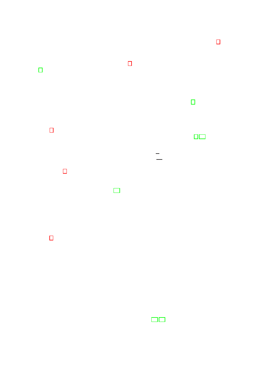
Figure 6: Pseudo-triangle and 2-convex partition

Two other natural questions for k-convex n-gons are decomposing them into few

convex pieces in terms of k, as well as giving a bound on the number of pieces of the
convex hull minus the polygon. However, in both cases the answer is unrelated to k,
because the polygon in Figure 7 (left) is 2-convex yet requires n

− 2 convex pieces, which

is obviously tight because every polygon can be triangulated. On the other hand, the
polygon in Figure 7 (right) is also 2-convex and has

pockets, which is tight because

two consecutive points on the convex hull are at least two edges apart if they are not
adjacent on the polygon boundary.

2.2

Recognition complexity

Let us start our considerations by observing that the stabbing number of a polygon with
n vertices can be easily found in O(n

) time, as follows. The standard duality transform

maps each edge of the polygon to a double wedge consisting of lines through a common
point, not including the vertical; the two lines that bound this dual wedge correspond to
the endpoints of the primal segment. In the primal, any point inside a wedge is a line
that stabs the segment. Therefore, the primal line that would stab most segments is in
the dual a point that belongs to as many double wedges as possible—a maximum depth
problem that can easily be solved by constructing the arrangement and then traversing
its cells.

The obtained O(n

) time bound is essentially tight, as in this section we prove that

finding the stabbing number of a polygon, or, equivalently, finding the smallest k for
which the polygon is k-convex, is a 3SUM-hard problem. This family of problems is

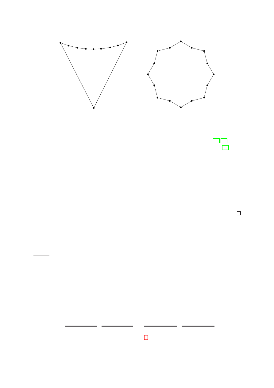
Figure 7: A polygon with many convex pieces (left) and many pockets (right).

widely believed to have an Ω(n

) lower bound for the worst case runtime [17, 19]. We

start by giving the following result, which follows directly from Theorem 4.1 in [17].

Lemma 2.

For every integer a, let us consider the point p

= (a, a

) on the cubic y = x

Then if a, b, c are distinct integers, p

, p

are collinear if and only if a + b + c = 0.

Proof. The points p

, p

are collinear if and only if the determinant

a a

b b

c c

= (b

− a)(c − a)(c − b)(a + b + c)

vanishes, which, the numbers being different, happens exactly when a + b + c = 0.

We next show that the points p

with x

∈ Z on the cubic y = x

can be replaced by

infinitesimally small vertical segments S

with upper endpoint p

, such that three of them

can be stabbed by a single line if and only if their three upper endpoints are collinear.

Lemma 3.

Let m, a, b, c, M be five integers such that m < a < b < c < M. Let ε =

6(M −m)

and let s

be the (vertical) segment with endpoints p

= (t, t

) and p

′

= (t, t

− ε).

Then s

, s

and s

can be stabbed by a single line if and only if p

, p

, and p

are collinear.

Proof. Assume that the points p

, p

are not collinear, and let us take three points

= (a, a

− ε

), q

= (b, b

− ε

), q

= (c, c

− ε

), with 0

≤ ε

, ε

≤ ε, i.e., three points

on the segments s

, s

and s

. The points q

, q

would be collinear if and only if the

determinant

a a

− ε

b b

− ε

c c

− ε

a a

b b

c c

−ε

= (b

− a)(c − a)(c − b)(a + b + c)

}

+ ε

− c) − ε

− c) + ε

− b)

}

is 0, but this is impossible because by Lemma 2, z is an integer different from 0, which
cannot become 0 by the addition of δ, because

|ε

− c) − ε

− c) + ε

− b)| ≤ |ε

− c)| + |ε

− b)| ≤ ε · 3(M − m) =

1
2

Theorem 1.

The problem of finding the stabbing number of a polygon is 3SUM-hard.

Proof. The 3SUM problem is defined as follows: Given a set S of n integers, do there
exist three elements a, b, c

∈ S such that a + b + c = 0? We will prove below that this

problem can be reduced in O(n log n) time to the problem of computing the stabbing
number of an n-gon. In other words, using the notation in [17],

3SUM ≪

(n log n)

stabbing number of a polygon.

Let x

, . . . , x

be the input integers. We proceed to the reduction by steps.

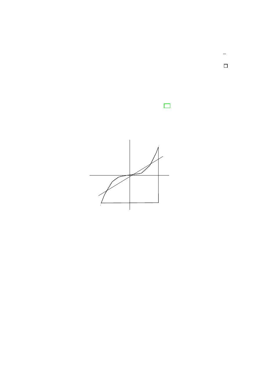
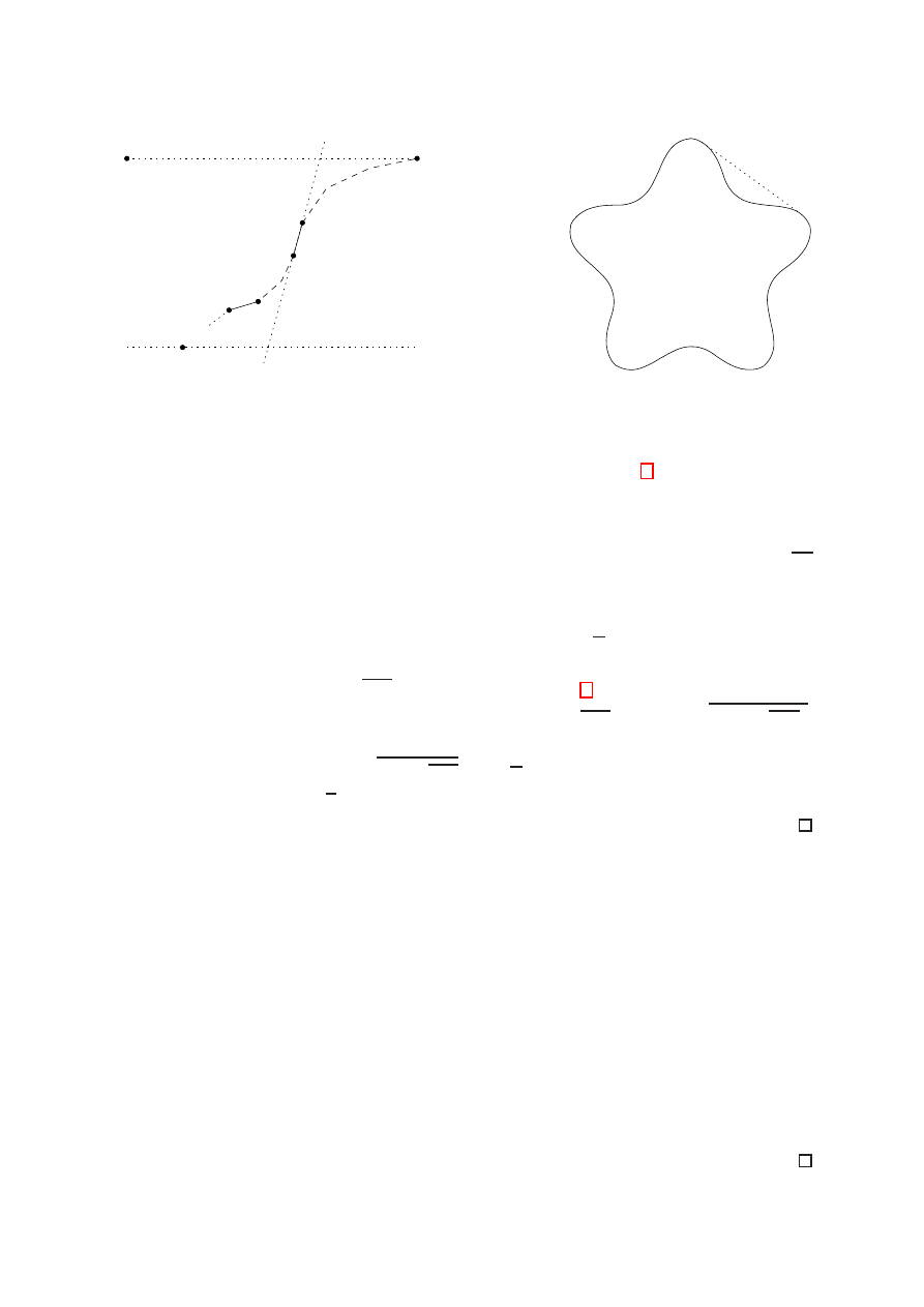
Figure 8: Polygon P

with vertices on the cubic y = x

(dashed). The scale of the axis is

not 1 : 1, to make the figure visible.

Step 1

. Sort the input numbers; let y

≤ y

≤ · · · ≤ y

be the resulting list,

L. This step

is done in O(n log n) time.

Step 2

. If 0 appears thrice in

L, exit with a sum of three numbers in the input being 0,

otherwise continue. The step is completed in linear time.

Step 3

. If a

6= 0 appears at least twice in L, check whether −2a ∈ L. If so, exit with a

sum of three numbers in the input being 0, otherwise continue. The step is completed
in O(n log n) time, as binary search can be used in the sorted list (in fact, O(n) time is
sufficient by scanning the list from left to right and from right to left, in a coordinated
simultaneous advance).

Step 4

. Remove multiples from the list

L so that each number appears exactly once. This

requires linear time. Let a

< a

· · · < a

(where t

≤ n) be these numbers.

Step 5

. Define m = a

−1, M = a

+1, and q = (M, m

). Now let us consider the polygon

whose vertices, described clockwise, are p

. . . p

q, where p

= (x, x

), as in

= (a, a

)

′
a

= (a, a

− ε)

= (a + ε

(a + ε

)

= (a − ε

(a − ε

)

Figure 9: Polygon P

with vertices on the cubic y = x

replaced by infinitesimal vertical

slots.

the preceding lemma (Figure 8). Observe that the stabbing number of P

is 4, and that

the polygon can be constructed in O(n) time.

Step 6

. Next we modify the polygon P

to become the polygon P

whose vertices, de-

scribed clockwise, are p

′

. . . u

′

q, where p

′

= (x, x

− ε), u

− ε

, (x

− ε

)

), v

= (x + ε

, (x + ε

)

)); see Figure 9. This polygon can be constructed

in O(n) time, and in the vicinity of the point p

its stabbing number changes locally from

1 to 3; see Figure 10. Let s

be the segment joining u

to p

′

. Therefore, the stabbing

number of P

is 12 if and only if three of the segments s

can be simultaneously stabbed,

and 8 otherwise, as two of those segments can always be stabbed.

Figure 10: From P

to P

the stabbing number locally increases from 1 to 3.

Step 7

. Compute the stabbing number of polygon P

using the best possible algorithm.

Step 8

. If the stabbing number of polygon P

is 10, conclude that there were three

numbers in the initial input such that their sum is 0; if the stabbing number of P

is 8,

conclude that there are no such three numbers.

The correctness of Step 8 is a direct consequence of Lemma 2 and Lemma 3. As

all steps but Step 7 have overall complexity O(n log n), we conclude that Step 7, the
computation of the stabbing number of a polygon, is a 3SUM-hard problem, as claimed.

As an immediate consequence we obtain:

Corollary 1.

The problem of deciding the smallest number k such that a given polygon

is k-convex is 3SUM-hard.

Also, if we replace Step 7 in the proof of Theorem 1 by checking whether or not

polygon P

is 4-convex, we get:

Corollary 2.

The problem of deciding whether a given polygon is 4-convex is 3SUM-hard.

2.3

Fast triangulation

Triangulating a simple polygon faster than in O(n log n) time with a simple method is a
challenging open problem. For k-convex polygons, this can be achieved, by the fact that
we can sort the vertices of a k-convex polygon P in any given direction (say, x-direction)
in O(kn) time: Simply scan around ∂P and use insertion sort, starting each time from
the place where the x-value of the previous vertex has been inserted. Then any fixed
value x

, once being inserted, takes part in later comparisons at most 2k

− 1 times because

otherwise, the vertical line x = x

would intersect P in more than k components. Having

x-sorted P ’s vertices, a simplified plane sweep method can be used to build a vertical
trapezoidation [9, 16] (and then a triangulation) of P . Only trivial data structures may
be used, as the scenario on the sweep line is of complexity O(k), by the k-convexity of P .
Thus, each vertex of P can be processed in O(k) time during the sweep. We conclude:

Proposition 1.

Any k-convex polygon can be triangulated in O(kn) time and O(n) space.

Using suitable data structures, a faster yet still implementable algorithm is possible,

as we show next. Call a polygon k-monotone if every vertical line intersects the interior
of the polygon in k intervals. (This property is implied by k-convexity, and is equivalent
to x-monotonicity for k = 1.) Actually, we do not even need the polygon to be simple, we
just need a sequence of x-coordinates such that every other x-coordinate comes between
at most 2k consecutive pairs of x-coordinates.

Lemma 4.

The vertices of any k-monotone polygon can be x-sorted in O(n log(2 + k))

time.

Proof. We use a binary insertion sort, in which we add the points in order along the
polygon into a balanced binary search tree. The binary search tree has the dynamic
finger property: inserting an element that has rank r different from the previously inserted
element costs only O(log(2 + r)) time. (For example, splay trees [30] and Brown & Tarjan
finger trees [7] both have this property.) Once the elements are inserted into the binary
search tree, we simply perform a linear-time in-order traversal to extract them in sorted
order.

Now we find the bound on the total cost of the insertions. When we insert an element

of rank difference r from the previously inserted element, we can charge this cost to r
points formed from projecting all vertices onto all edges of the polygon. There are at
most O(nk) such points of projection, so the total number of charges is at most O(nk).
Thus the total insertion cost is O(

n
i

log(2 + r

)) where

n
i

= O(nk). Such a

sum is maximized when the r

are all roughly equal, which means that they are all

Θ((nk)/n) = Θ(k). Therefore the total cost is at most O(n log(2 + k)).

To see that this bound is optimal in the comparison model, consider the case in which

the polygon is a comb with k tines. Then sorting the x-coordinates is equivalent to
merging k sorted sequences of length n/k, which is known to take Θ(n log k) time in the
worst case.

Lemma 4 yields a fast triangulation method for general k-convex polygons. We first

sort the vertices of the k-convex polygon P in a fixed direction, in O(n log k) time. Again,
a plane sweep is used to compute a triangulation of P . As the intersection of P with the

sweep line is of complexity O(k) only, by the k-convexity of P , each of the n vertices of P
can be processed in O(log k) time during the sweep.

Theorem 2.

Any k-convex polygon can be triangulated in O(n log k) time and O(n)

space.

Two-Convex Polygons

3.1

Characterization

In this section we give a characterization of 2-convex polygons that allows their recognition
in time O(n log n), and a description of their structure that will be used later in several
of our results.

We observe that k-convexity is a property that may be lost by small perturbations on

the positions of the vertices of a polygon. For example, small changes in the positions of
the vertices p

, . . . , p

in Figure 4, could yield a 1- or 2-convex polygon. As a consequence,

stabbing a polygon along its edges will not, in most cases, give enough information for
deciding its k-convexity.

Figure 11: Constructing an inner tangent

Let P be a simple polygon, and denote its boundary by ∂P . A line L is called a

j-stabber of P if L crosses ∂P at least j times. Note that a j-stabber may contain whole
edges of P ; these are not considered to contribute to the count. An edge of a polygon P
is called an inflection edge if it joins a convex and a reflex vertex of P . An inner tangent
of P is a line segment T

⊂ P that contains two non-adjacent reflex vertices of P in its

relative interior; see Figure 11.

Lemma 5.

A simple polygon P is 2-convex if and only if P has no inner tangent, and

no 3-stabber that contains an inflection edge.

Proof. Consider the ‘only if’ implication first. Suppose that for some inflection edge e
of P , its supporting line L is a 3-stabber for P . Then a slight perturbation of L gives
rise to a line L

′

that crosses ∂P at least two more times than L does. One of these extra

crossings lies in the interior of e, and one on the second edge of P incident to the reflex
vertex of e. Thus P admits a 6-stabber, and therefore P cannot be 2-convex. Similarly,
if P has some inner tangent T , defined by reflex vertices u and v, say, then a 6-stabber
cutting off u and v exists in the vicinity of T .

′

Figure 12: Constructing a 3-stabber

To prove the ‘if’ implication, assume that P is not 2-convex. Then there exists a

6-stabber L of P . Let c

, . . . , c

denote six consecutive crossings of L with ∂P such that

the line segment joining c

to c

is contained in P . Two types of crossing pattern arise, as

shown in Figures 11 and 12, respectively. In the former case, we simply connect the two
crossings c

and c

with a geodesic path inside P (dashed), and obtain an inner tangent

(bold). In the latter case, if an inner tangent exists locally, then we can construct it
in a similar way, possibly by moving the geodesic’s endpoints from c

and c

closer to

each other along ∂P . Otherwise (as Figure 12 illustrates) we can find an inflection edge
(bold) between c

and c

whose supporting line L

′

crosses P ’s boundary twice between c

and c

. But the line L

′

has to cross ∂P once more, and thus it is a 3-stabber containing

an inflection edge, which is not possible.

3.2

Recognition

Suppose that we want to decide if a polygon P is 2-convex. (Assume that P is not convex;
the problem is trivial, otherwise.) Our recognition algorithm is based on Lemma 5. We
look for inner tangents and 3-stabbers at inflection edges. To this end, we first shoot two
rays at each reflex vertex v of P in the directions determined by the edges of P incident
with v. This can be done in O(n log n) [8]. If ∂P is intersected more than once by any of
these rays, then a 6-stabber exists, and we report that P is not 2-convex.

Suppose then that each ray shot at the reflex vertices of P yields a unique intersection

point with ∂P . We store the points of intersection and use them to check for inner
tangents. Define, for each reflex vertex v of P , its critical range C(v) as the set of all
points x

∈ ∂P such that xv can be prolonged to a line segment tangent to P at v. Note

that such a segment need not lie entirely in P . However, C(v) consists of exactly two
connected intervals on ∂P whose endpoints are among the stored points obtained from
ray shooting. See Figure 13, where C(v) is drawn with bold lines.

Lemma 6.

P admits an inner tangent if and only if P has two reflex vertices v and v

′

such that v

∈ C(v

′

) and v

′

∈ C(v).

Proof. Clearly, if two vertices v and v

′

define an inner tangent for P , then v

∈ C(v

′

) and

′

∈ C(v) hold. Conversely, assume that both inclusion conditions are fulfilled. Consider

the geodesic path π between v and v

′

inside P . Either π is the line segment vv

′

, and thus

can be extended to an inner tangent at v and v

′

, or π detours via reflex vertices w

, . . . , w

Figure 13: Critical range for vertex v

In the latter case (which is illustrated in Figure 14), we can extend the line segments vw

and w

′

to inner tangents, because ray shooting at reflex vertices of P has led to unique

intersection points with ∂P , and thus the path π does not cross the four (dashed) rays
depicted in the figure.

′

Figure 14: Geodesic path between v and v

′

The strategy for detecting inner tangents is now clear. First we associate to each reflex

vertex v two intervals, each containing a set of consecutive vertices of P lying within the
critical range of v. We then choose a point x in ∂P and calculate the set R(x) of reflex
vertices containing x in their critical ranges. We then slide x along ∂P , maintaining the
set R(x) in a range search tree. R(x) has to be updated each time x passes over a point
of intersection of ∂P with a ray shot from a reflex vertex of P . Moreover, when x reaches
some reflex vertex v of P , we check in logarithmic time whether the intervals previously
associated to v contain any element in R(v). Thus this phase takes O(n log n) time.

Since range search trees can be implemented in linear space, we have the following

result:

Theorem 3.

Deciding if a simple polygon P with n vertices is 2-convex can be done in

O(n log n) time and O(n) space.

3.3

Shape structure

We have given a geometric characterization of 2-convex polygons, in Subsection 3.1. The
present subsection aims at giving a qualitative description of their shape.

Lemma 7.

Let P be a 2-convex polygon. Let C = p

. . . p

be the chain of vertices that

connects (counterclockwise) two consecutive vertices p

, p

on the convex hull CH(P ).

Then C can be partitioned into three chains C

= p

. . . p

, C

= p

. . . p

, and C

. . . p

, for 0

≤ r ≤ s < t, such that all vertices in C

and C

are convex (in P ), while

all vertices in C

are reflex.

Proof. If C

is empty, the lemma is obviously true, so we assume that the chain C contains

at least one reflex vertex. Let p

be the last point of the chain C to be hit in a parallel

sweep starting with the line defined by p

which, without loss of generality, we assume

to be horizontal. Observe that p

is necessarily a reflex vertex. Let us recall that an

inflection edge is adjacent to a reflex vertex and to a convex vertex and that, according
to Lemma 5, 2-convex polygons do not have 3-stabbers containing an inflection edge. We
are going to see that there is at most one inflection edge in the chain p

. . . p

, and that

the same applies to the chain p

. . . p

. Let p

be the first inflection edge starting from

(see Figure 15.a). As the directed ray p

intersects the chain p

at least once, the

chain p

is necessarily to the right of the oriented line p

. Observe that p

is to

the right of the oriented line p

, because otherwise a rotation around p

starting from

i−1

will define an inner tangent, forbidden in 2-convex polygons according to Lemma 5.

Finally, if we assume that there exists a convex vertex p

in the chain p

, then we

have that p

j−1

is an inflection edge supporting a 3-stabber: the ray p

j−1

intersects

the polygon at least once, while the ray p

j−1

intersects the chain p

and therefore

intersects the polygon at least twice.

Observe that the chains C

and C

might be singletons in some cases, and that C

might be empty. However, the generic aspect of a pocket and the shape of a 2-convex
polygon are as shown in Figure 15.b). The next result follows directly:

Corollary 3.

If the convex hull of a 2-convex polygon P has k vertices, then the boundary

of P can be decomposed into 2k convex chains.

The Erd˝os-Szekeres Theorem says that every set of n points in general position con-

tains at least log n points that are in convex position, and that this value is asymptotically
tight [12]. As every point set can be ‘polygonized’, one cannot expect a better value when
the points are chosen from the set of vertices of an arbitrary polygon. However, when
a point set is the set of vertices of a 2-convex polygon, we can improve this bound as
follows.

Theorem 4.

Every 2-convex polygon with n vertices has a subset of

⌈

n/2

⌉ vertices in

convex position. This bound is tight.

Proof. By Corollary 3, the boundary of a 2-convex polygon with k vertices on its convex
hull can be decomposed into at most 2k convex chains. If k

≥ ⌈

n/2

⌉, we are done,

otherwise one of the 2k convex chains necessarily has size at least

⌈

n/2

⌉. The amoeba-

like example in Figure 15.b), with k =

⌈

n/2

⌉ vertices in the convex hull and 2k convex

chains of equal size shows that this bound is tight.

i+1

j−1

Figure 15: Illustration for the proof of Lemma 7.

We conclude this section with a consequence of the preceding theorem.

Corollary 4.

If an n-gon is 2-convex, then its vertices can be grouped into at most 2

√

subsets, each in convex position.

Proof. Let S(n) be the number of convex subsets needed to partition the vertex set of a
2-convex polygon with n vertices. We show that S(n)

≤ α

√

n by induction over n. The

induction base for n = 3 is obvious, and valid for any α

≥ 1. By Theorem 4 we find one

convex subset of size at least

⌈

n/2

⌉. Moreover, by Lemma 1, the remaining points define

also a 2-convex polygons and we have S(n)

≤ 1 + S(⌊n −

n/2

⌋) ≤ 1 + α

⌊n −

n/2

⌋,

where the last inequality comes from the induction hypothesis. To prove the lemma it

is sufficient to show that 1 + α

−

n/2

≤ α

√

n. Standard manipulation shows that

this is true for any α

≥ 2

√

2 and any n

≥ 1.

General

k-Convex Domains

The union or intersection of simple polygons may not be a polygon. In view of this fact,
the issue of how the degree of convexity behaves with respect to these operations is not
meaningful for this class of objects. In this section, we consider larger classes of sets in R

for which these natural questions may be discussed. We first study some properties of
general (not necessary polygonal) subsets of R

Lemma 8.

The union of a k-convex set Q

and an m-convex set Q

is a (k + m)-convex

set, which is tight.

Proof. The number of intersections of a line with the boundary of Q

∪Q

can be at most

2k + 2m. On the other hand, if Q

and Q

are disjoint and the line that gives k and m

connected components, respectively, is the same, the value is achieved.

Figure 16: Intersecting k-convex sets

Lemma 9.

The intersection of a k-convex set Q

and an m-convex set Q

is a (k+m

−1)-

convex set, which is tight.

Proof. An oriented line will cut the boundary of Q

at most 2k times and the boundary

of Q

at most 2m times. However, the first intersection point a does not contribute to

the total number of cuts with Q

∩ Q

unless a

∈ Q

∩ Q

, in which case it contributes

only once instead of twice as intersection. The same happens with the last point, which
gives the upper bound. An example proving the tightness appears in Figure 16(a).

Corollary 5.

The intersection of a family of m k-convex sets is a (m(k

− 1) + 1)-convex

set, which is tight.

Proof. The upper bound follows from the preceding theorem, and a construction giving
its tightness is shown in Figure 16(b).

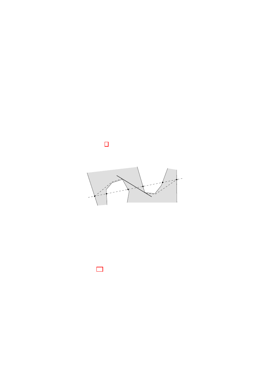
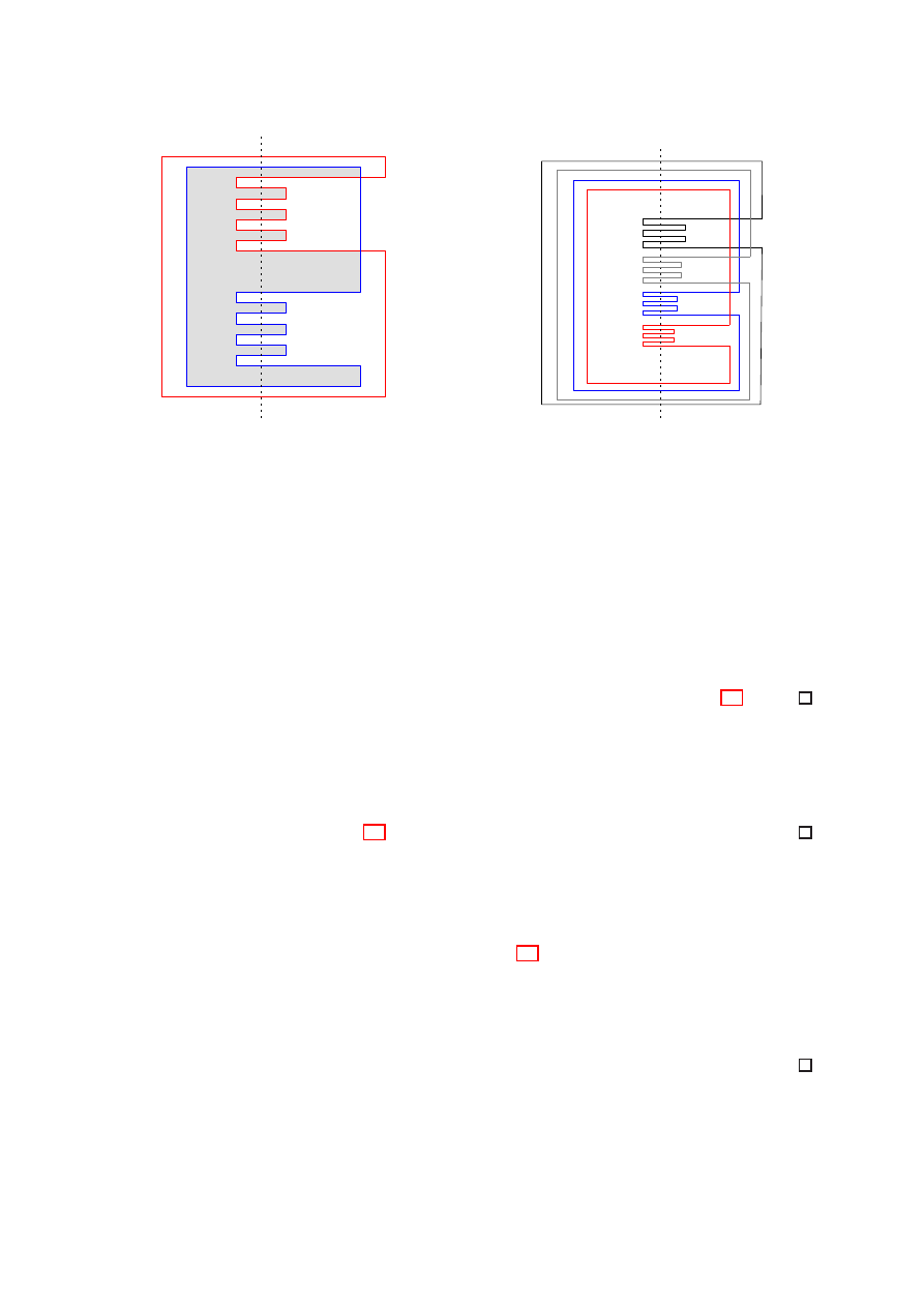
Theorem 5.

There is no Helly-type theorem for k-convex sets.

Proof. We are constructing a family of m 2-convex sets such that any subfamily has
nonempty intersection yet there is no point common to all of them. Let Q

be a regular

polygon with m edges e

, . . . , e

(refer to Figure 17). Let P

∗

be the polygonal chain

obtained from the boundary of Q

by removing edge e

and an infinitesimal portion of

i−1

and e

. Finally, let us give some slight thickness to the chain so it becomes a

polygon P

. Notice that the polygons P

, . . . , P

are 2-convex, the intersection

m
i

clearly empty, while the intersection of every proper subfamily F is nonempty because it
contains the intervals e

for all those P

6∈ F .

The preceding lemmas apply to k-convex sets in general, not only polygonal domains.

(A polygonal domain is a set obtained by a finite number of union operations of simple
polygons.) However, a significant difference appears in our next results, that are possibly

Figure 17: No Helly-type theorem for k-convex sets

the most natural to explore, because they involve transversal lines, which are precisely
the main concept underlying the definition of k-convexity.

Let us recall [36] that given a family of sets Q

, . . . , Q

, a line ℓ is said to be a

transversal of the family if ℓ has a nonempty intersection with each of the sets. When the
sets are convex, the ordering in which they are traversed (disregarding the orientation of
the line) is called a geometric permutation, a topic that has received significant attention
[36]. In particular, it has been proved that m compact disjoint convex sets admit at most
2m

− 2 geometric permutations, which is tight [10].

Let us consider now transversals of compact 2-convex sets. Notice that every object

will appear at least once, but may appear twice on the transversal, which we consider as
combinatorially different cases of the associated generalized geometric permutation. What
is the maximum number of generalized geometric permutations a family of m 2-convex
sets may have?

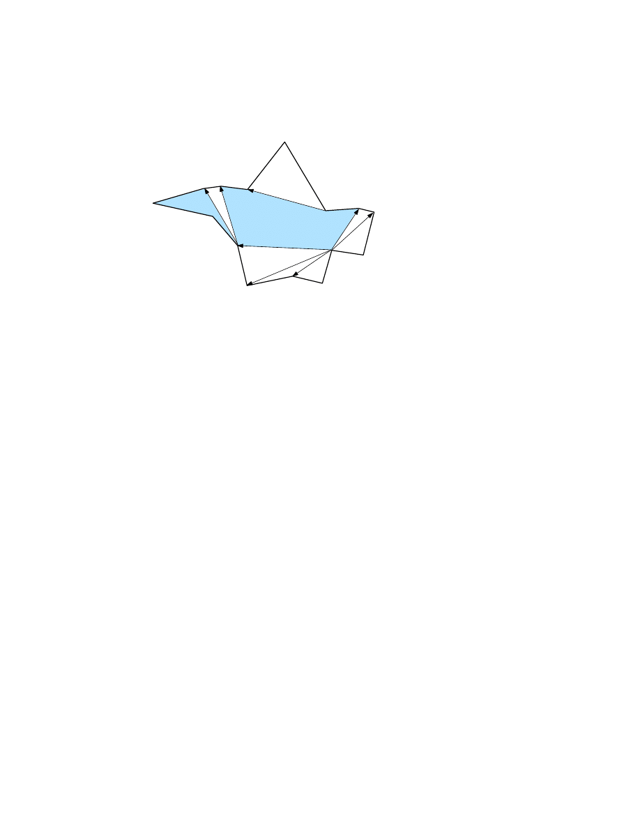
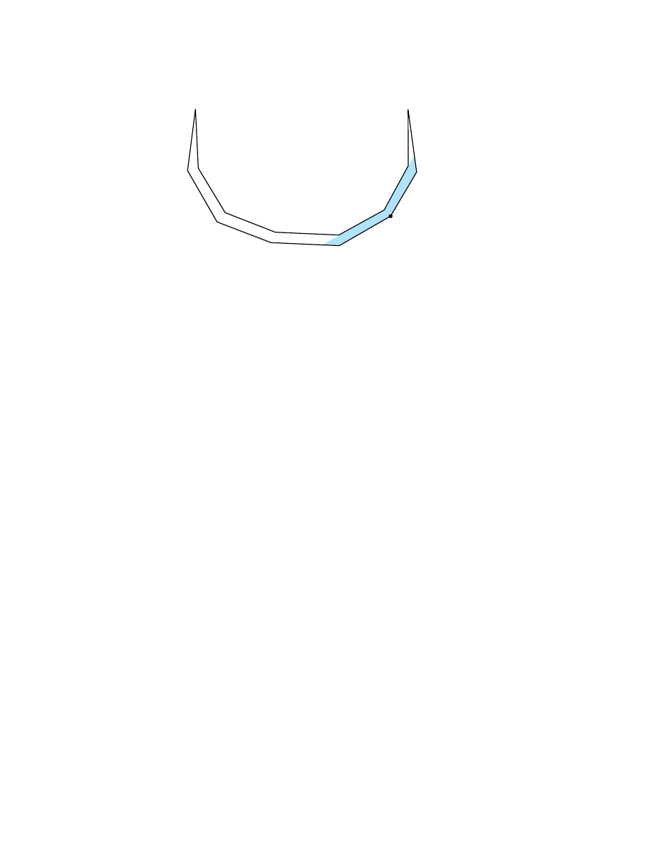
Theorem 6.

The number of generalized geometric permutations of a set of m 2-convex

objects may be exponential in m.

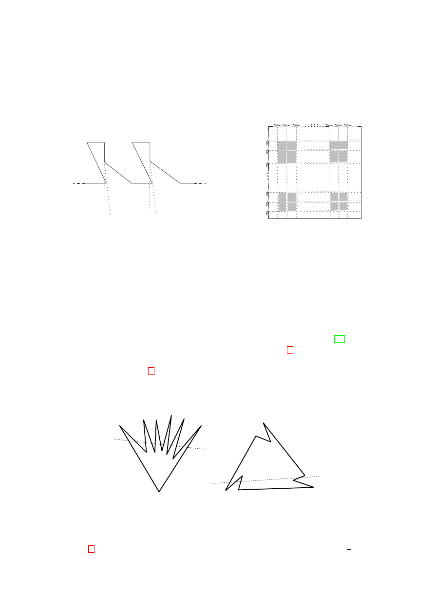
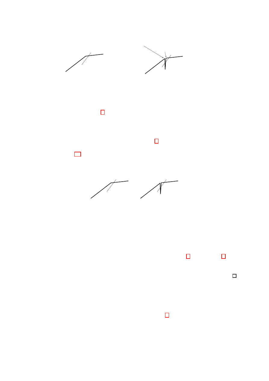
Proof. We first show that a 2-convex objects can be arbitrarily complex. A nose of an
object O is a zig-zag sequence of a reflex and a convex vertex of the boundary of O as
depicted in Figure 18(a). Locally a line ’normal’ to the nose intersects O in two connected
components. The shaded area in Figure 18(a) indicates the region which is not intersected
by a line tangent to one of the vertices of the nose. Thus we can iteratively construct
further noses in this region without destroying the 2-convexity of O. Figure 18(b) shows
an example where the principle shape of O is part of a disk. Observe that when the
radius of the disk is large enough we can arrange an arbitrary number of flat noses such
that O stays 2-convex.

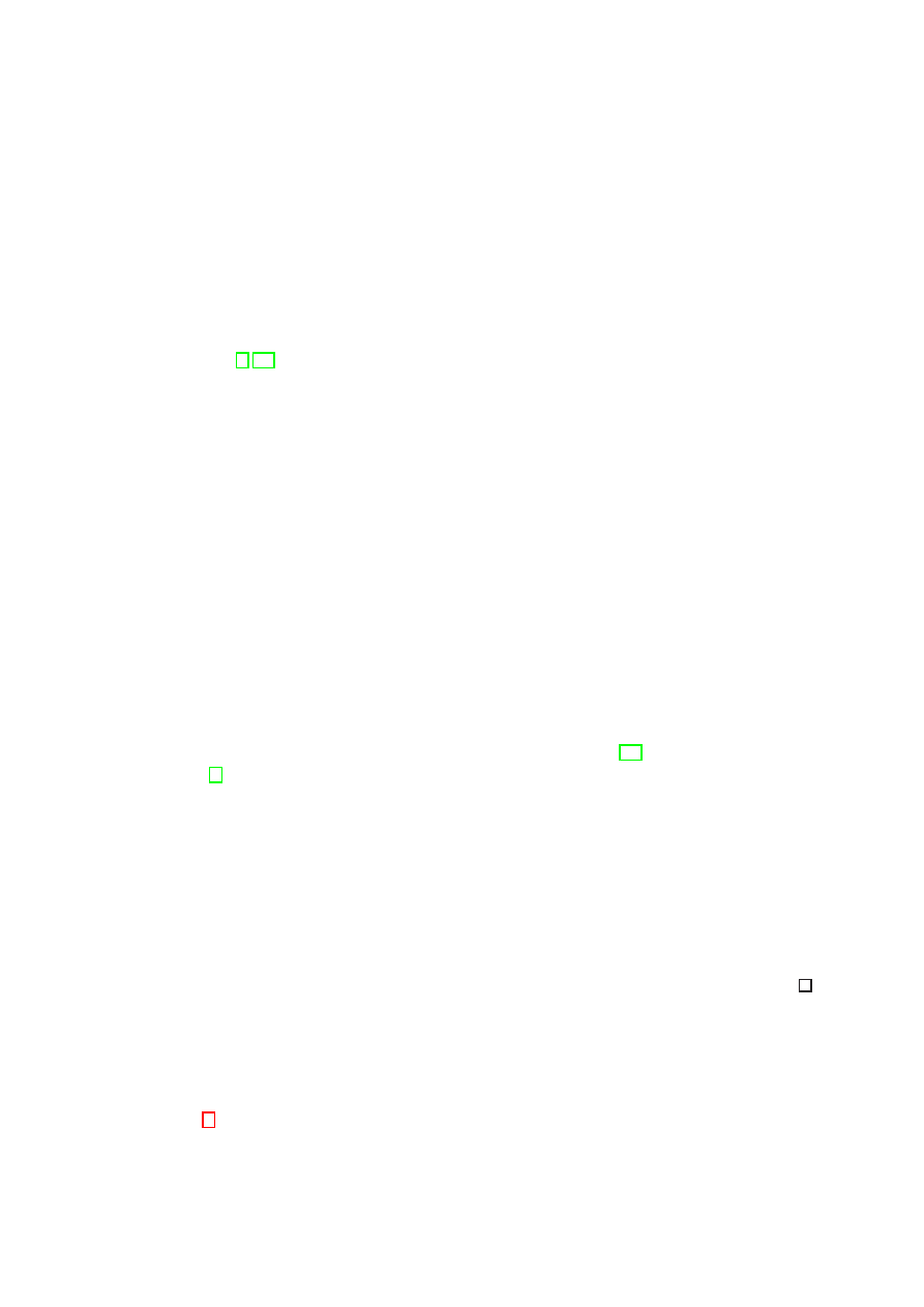
Let R

be an object which has the base shape of an axis-aligned rectangle, where the

left side is actually part of a circle with sufficiently large radius and a center point far to
the right of R

. We place 2

i−1

noses along this side, so that R

stays 2-convex as described

above. Next we arrange k objects R

to R

from left to right, as depicted in Figure 18(c)

for k = 3. We position the noses for each R

in a regular way such that a rotating line

(a)

(b)

(c)

ABBC

ABC

AABBCC

AABBC
AABCC
AABC

ABBCC

ABCC

Figure 18: (a) and (b): 2-convex objects can have an unbounded number of noses. (c):
The number of generalized geometric permutations for a set of 2-convex objects can be
exponential.

∗

Figure 19: The number of generalized geometric permutations for a set of 2-convex
polygons can be quadratic.

(see the dashed lines in Figure 18(c)) intersects the noses in the same manner as the
digit “1” shows up in the sequence of all 2

binary numbers of length k. Thus, we get

different generalized geometric permutations for this setting, as each object appears

twice if the nose is intersected, but only once otherwise.

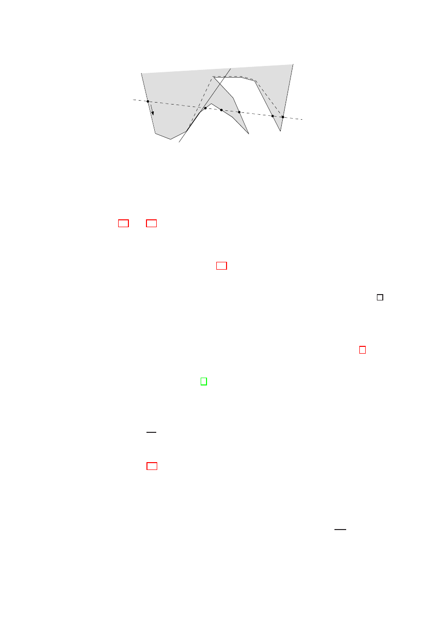
Theorem 7.

The maximum number of generalized geometric permutations of a set of

2-convex polygonal domains with a total of n boundary edges is Θ(n

Proof. As the standard duality transform maps each edge to a double wedge, the induced
arrangement of 2n lines in the dual plane yields a quadratic number of cells that bound
from above the number of possible ways of stabbing the set of objects.

To see that the bound is asymptotically tight, we give a construction using n 2-

convex polygons; in fact, the simplest possible ones, namely, nonconvex quadrilaterals.
Let Q

∗

= a

∗

be the quadrilateral shown in Figure 19. Let h be a horizontal line

through a

∗

and let Q

∗

= a

∗

be translates of Q

in such a way that all of them

are pairwise disjoint and a

∗

, a

∗

, . . . , a

∗

appear in this order on h. Finally, let us perturb

infinitesimally a

∗

to a

in such a way that

a) points a

, a

, . . . , a

are in general position,

b) for all i, j, k, with i

6= j, the line a

leaves above the point c

and below the point

For i = 1, . . . , n, let Q

be the quadrilateral with vertices a

. There are

lines of

the type a

; each of them leaves above and below a different set of points a

, and is a

transversal because it crosses all the segments b

for every k. Now, if a

is below the

transversal, Q

is intersected once, while if a

is above the transversal, Q

is intersected

twice. Therefore, we have obtained

generalized geometric permutations.

Observe that the two preceding theorems apply mutatis mutandis to k-convex sets,

because 2-convex sets are also k-convex for k

≥ 3.

Discussion and Open Problems

In this paper we have considered a new concept of generalized convexity. Moving from
convexity to 2-convexity is seemingly a small change, as we are just accepting lines to
intersect in at most two connected components instead of one. It is remarkable that this
modest departure has strong consequences in the complexity of the new class of objects,
as we have seen in this paper; obviously, even more when the degree of convexity is
increased. Several open problems remain and many interesting questions can be raised.
We list some of them below.

a) Can the recognition of 2-convex polygons be carried out in linear time, improving

on the O(n log n) algorithm we provide?

b) Finding the smallest k such that a given polygon is k-convex is a 3SUM-hard prob-

lem. In particular, recognizing 4-convexity is already 3SUM-hard. We do not know
whether the situation is the same for 3-convexity or whether a subquadratic time
algorithm exists for this case.

c) Is it possible to generalize Theorem 4? For example, is it true that every k-convex

polygon with n vertices has a large subset of vertices that are the vertices of a
(k

− 1)-convex polygon?

d) Let us define the k-convex hull of a point set S as the smallest area polygon which

is k-convex, has a subset T

⊂ S as vertex set and every point in S r T is inside the

polygon. Which is the complexity of computing this k-convex hull? Observe that
for k = 1 this notion is the usual convex hull of a point set.

e) Give combinatorial bounds and efficient algorithms for decomposing a polygon into

k-convex subpolygons. This is a classical problem when convex subpolygons are
considered [18] and also the decomposition into pseudotriangles, which are 2-convex
polygons, has been studied [28]. However, the latter result might be improved by
considering more general 2-convex polygons.

f) A k-convex decomposition of a set S of n points in the plane is a decomposition

of its convex hull into k-convex polygons such that every point in S is a vertex of
some of the polygons. For k = 1, a triangulation suffices, though it has been proved
that if we allow arbitrary convex sets the number can be reduced [24]. On the
other hand, it has been shown that there exist always a decomposition into exactly
n

− 2 pseudotriangles, which are 2-convex polygons [28]. It is an intringuing open

problem to decide whether this number can be reduced to sublinear if we allow
arbitrary 2-convex polygons.

Finally, let us mention that in this paper we have focused on k-convex polygons. It is

natural to define a similar concept for finite point sets, namely, being in k-convex position,
where k is given by the smallest degree of convexity attained when all possible polygoniza-
tions of the point set are considered. This issue is considered in a companion paper [2].

Acknowledgements

We would like to thank Thomas Hackl, Clemens Huemer, David

Rappaport, Vera Sacrist´an and Birgit Vogtenhuber for sharing discussions on this topic.

References

[1] O. Aichholzer, R. Fabila-Monroy, D. Flores-Pe˜

naloza, T. Hackl, C. Huemer, J. Urru-

tia, and B. Vogtenhuber. Modem Illumination of Monotone Polygons. In Proc. 25th
European Workshop on Computational Geometry EuroCG ’09, Brussels, Belgium,
2009, 167-170.

[2] O. Aichholzer, F. Aurenhammer, T. Hackl, F. Hurtado, P.A. Ramos, J. Urrutia, P.

Valtr, B. Vogtenhuber. k-convex points sets. Manuscript, 2010.

[3] O. Aichholzer, C. Huemer, S. Kappes, B. Speckmann, C.D. T´oth. Decompositions,

partitions, and coverings with convex polygons and pseudo-triangles. Graphs and
Combinatorics 23 (2007), 481-507.

[4] G. Aloupis, P. Bose, V. Dujmovic, C. Gray, S. Langerman, B. Speckmann. Triangu-

lating and guarding realistic polygons. Proc. 20

Canadian Conference on Compu-

tational Geometry, 2008.

[5] D. Artigas, M.C. Dourado, J.L. Szwarcfiter. Convex partitions of graphs. Electronic

Notes in Discrete Mathematics 29 (2007), 147-151.

[6] M. Breen, D.C. Kay. General decomposition theorems for m-convex sets in the plane.

Israel Journal of Mathematics 24 (1976), 217-233.

[7] M.R. Brown, R.E. Tarjan. Design and Analysis of a Data Structure for Representing

Sorted Lists. SIAM Journal on Computing 9(3) (1980), 594-614.

[8] B. Chazelle, H. Edelsbrunner, M. Grigni, L. Guibas, J. Hershberger, M. Sharir, J.

Snoeyink. Ray shooting in polygons using geodesic triangulations. Algorithmica 12
(1994), 54-68.

[9] B. Chazelle, J. Incerpi. Triangulation and shape-complexity. ACM Transactions on

Graphics 3 (1984), 135-152.

[10] H. Edelsbrunner, M. Sharir. The maximum number of ways to stab n convex non-

intersecting sets in the plane is 2n

− 2 Discrete Comput. Geom. 5 (1990), 35ˆu42.

[11] H. ElGindy, G.T. Toussaint. On geodesic properties of polygons relevant to linear

time triangulation. The Visual Computer 5 (1989), 68-74.

[12] P. Erd˝os, G. Szekeres. A combinatorial problem in geometry. Compositio Mathemat-

ica, 2 (1935), 463-470.

[13] R. Fabila-Monroy, Andres Ruis Vargas, and J. Urrutia. On Modem Illumination

Problems. XIII Encuentros de Geometria Computacional, Zaragoza, Espa˜

na, June

29 - July 1 2009, 9-19.

[14] S.P. Fekete, M.E. L¨

ubbecke, H. Meijer. Minimizing the stabbing number of match-

ings, trees, and triangulations. Proc. 15

Ann. ACM-SIAM Symp. on Discrete

Algorithms, 2004, 430-439.

[15] E. Fink, D. Wood. Fundamentals of restricted-orientation convexity. Information

Sciences 92 (1996), 175-196.

[16] A. Fournier, D.Y. Montuno. Triangulating simple polygons and equivalent problems.

ACM Transactions on Graphics 3 (1984), 153-174.

[17] A. Gajentaan and M. H. Overmars. On a class of O(n

) problems in computational

geometry. CGTA: Computational Geometry: Theory and Applications, 5, (1995),
165-185.

[18] M. Keil. Polygon Decomposition in Handbook of Computational Geometry (2000),

491-518.

[19] J. King. A Survey of 3SUM-Hard Problems. http://www.cs.mcgill.ca/

∼jking/

[20] G. Kun, G. Lippner. Large empty convex polygons in k-convex sets. Periodica Math-

ematica Hungarica 46 (2003), 81-88.

[21] D.T. Lee, F.P. Preparata. An optimal algorithm for finding the kernel of a polygon.

Journal of the ACM 26 (1979), 415-421.

[22] A. Maheshwari, J.-R. Sack, H. Djidjev. Link distance problems. In: Handbook of

Computational Geometry, J.-R. Sack and J. Urrutia (eds.), Elsevier, 2000, 519-558.

[23] J. Matou˘sec, P. Plech´a˘c. On functional separately convex hulls. Discrete & Compu-

tational Geometry 19 (1998), 105-130.

[24] V. Neumann-Lara, E. Rivera-Campo, J. Urrutia. A note on convex decompositions

of point sets in the plane. Graphs and Combinatorics 20(2) (2004), 223-231.

[25] J. O’Rourke. Art Gallery Theorems and Algorithms. Oxford University Press, 1987.

[26] T. Pennanen. Graph-convex mappings and K-convex functions. Journal of Convex

Analysis 6 (1999), 235-266.

[27] G.J.E. Rawlins, D. Wood. Ortho-convexity and its generalizations. In: Computa-

tional Morphology, G.T. Toussaint (ed.), North-Holland Publishing Co., Amsterdam,
1988, 137-152.

[28] G. Rote, F. Santos, I. Streinu. Pseudo-triangulations—a survey. Contemporary

Mathematics 453 (2008), 343-410.

[29] S. Schuierer, D. Wood. Visibility in semi-convex spaces. Journal of Geometry 60

(1997), 160-187.

[30] D.D. Sleator, R.E. Tarjan. Self-adjusting binary search trees. Journal of the ACM

32(3) (1985), 652-686.

[31] J. Urrutia. Art Gallery and Illumination Problems. Handbook on Computational

Geometry, Elsevier Science Publishers, J.R. Sack and J. Urrutia eds. pp. 973-1026,
2000.

[32] F.A. Valentine. A three-point convexity property. Pacific Journal of Mathematics 7

(1957), 1227-1235.

[33] P. Valtr. A sufficient condition for the existence of large empty convex polygons

Discrete Comput. Geom., 28 (2002), 671ˆ

u682.

[34] G. Vegter. Kink-free deformations of polygons. Proc. 5

Ann. ACM Symp. Compu-

tational Geometry, 1989, 61-68.

[35] E. Welzl. On spanning trees with low crossing numbers. In: Data Structures and

Efficient Algorithms, B. Monien and T. Ottmann (eds.), Springer LNCS 594, 1992,
233-249.

[36] R. Wenger, Progress in geometric transversal theory. Contemporary Mathematics,

B. Chazelle and J.E. Goodman, Eds., American Math Society (1999), 375-393.

Document Outline

1 Introduction
2 k-Convex Polygons
3 Two-Convex Polygons
4 General k-Convex Domains
5 Discussion and Open Problems

Wyszukiwarka

Podobne podstrony:
Grunbaum etal Convexification of Polygons
Fortnow etal Complexity Limitations on Quantum Computation
More on hypothesis testing
ZPSBN T 24 ON poprawiony
KIM ON JEST2
Parzuchowski, Purek ON THE DYNAMIC
Foucault On Kant
G B Folland Lectures on Partial Differential Equations
free sap tutorial on goods reciept
5th Fábos Conference on Landscape and Greenway Planning 2016
ON CIĘ ZNA (fragm), WYCHOWANIE W CZAS WOJNY RELIGIJNEJ I KULTUROWEJ - MATERIAŁY, TEKSTY
Enochian Sermon on the Sacraments
Post feeding larval behaviour in the blowfle Calliphora vicinaEffects on post mortem interval estima
[30]Dietary flavonoids effects on xenobiotic and carcinogen metabolism
GoTell it on the mountain
Creative Writing New York Times Essay Collection Writers On Writing
Interruption of the blood supply of femoral head an experimental study on the pathogenesis of Legg C
CAN on the AVR

więcej podobnych podstron

Aichholzer etal On k Convex Polygons

Document Outline