Worm Propagation Modeling and Analysis

under Dynamic Quarantine Defense

Cliff Changchun Zou

Dept. Electrical &

Computer Engineering

Univ. Massachusetts

Amherst, MA

[e-mail]

Weibo Gong

Dept. Electrical &

Computer Engineering

Univ. Massachusetts

Amherst, MA

[e-mail]

Don Towsley

Dept. Computer Science

Univ. Massachusetts

Amherst, MA

[e-mail]

ABSTRACT

Due to the fast spreading nature and great damage of In-
ternet worms, it is necessary to implement automatic miti-
gation, such as dynamic quarantine, on computer networks.
Enlightened by the methods used in epidemic disease control
in the real world, we present a dynamic quarantine method
based on the principle “assume guilty before proven inno-
cent” — we quarantine a host whenever its behavior looks
suspicious by blocking traffic on its anomaly port. Then
we will release the quarantine after a short time, even if
the host has not been inspected by security staffs yet. We
present mathematical analysis of three worm propagation
models under this dynamic quarantine method. The analy-
sis shows that the dynamic quarantine can reduce a worm’s
propagation speed, which can give us precious time to fight
against a worm before it is too late. Furthermore, the dy-
namic quarantine will raise a worm’s epidemic threshold,
thus it will reduce the chance for a worm to spread out.
The simulation results verify our analysis and demonstrate
the effectiveness of the dynamic quarantine defense.

Categories and Subject Descriptors

K.6.5 [Management of computing and information
systems]: Security and Protection—Invasive software

General Terms

Security

Keywords

dynamic quarantine, worm propagation, epidemic model

1.

INTRODUCTION

Since the Morris worm in 1988 [9], the security threat

posed by worms has steadily increased, especially in the last

Permission to make digital or hard copies of all or part of this work for
personal or classroom use is granted without fee provided that copies are
not made or distributed for profit or commercial advantage and that copies
bear this notice and the full citation on the first page. To copy otherwise, to
republish, to post on servers or to redistribute to lists, requires prior specific
permission and/or a fee.
WORM’03, October 27, 2003, Washington, DC, USA.
Copyright 2003 ACM 1-58113-785-0/03/0010 ...

$

5.00.

several years. In 2001, the Code Red and Nimda infected
hundreds of thousands computers [10] [13], cost millions of
dollars loss to our society [16]. In January 2003, the SQL
Slammer worm spread out and infected more than 90% of
vulnerable computers within 10 minutes [12]. Fortunately,
none of them destroyed information on compromised hosts.
However, we cannot depend on the kindness of hackers in the
future. These worms have demonstrated how dangerous and
how fast a worm can spread to infect almost all vulnerable
computers on the Internet before human can take effective
counteractions. As the bandwidth of Internet connections
keeps increasing, future worms will require even less time to
finish the infection task.

For those fast spreading worms, human’s manual counter-

actions cannot catch up with the worms’ propagation speed.
Automatic mitigation is necessary for defending against fast
spreading worms in the future. Currently, the popular In-
trusion Prevention System (IPS) [8] on the security market
can be thought as a product combining intrusion detection
with primary automatic mitigation techniques.

Automatic mitigation is not very difficult for known worms.

Firewalls or routers can inspect packet contents according
to the signatures of known worms. A worm’s packets can be
dropped automatically when firewalls or routers find out the
signature of the worm. However, no signature is available
for an unknown worm — we have to rely on behavior-based
anomaly detection methods to detect an unknown worm.
The great challenge for automatic mitigation now is that the
current behavior-based anomaly detection methods have the
common problem of having high false alarm rate. If we rely
on automatic mitigation to block an unknown worm, it will
also block many legitimated connections or healthy comput-
ers. If we release the block on an alarmed host only after
security staffs check and find out that the host is healthy,
then many innocent healthy hosts will be blocked too long
due to human’s slow manual inspection.

Then how can we use current imperfect anomaly detection

systems to build an automatic mitigation defense against
fast spreading worms? Enlightened by the methods used
in epidemic disease control in the real world, we present a
dynamic quarantine method based on the principle “assume
guilty before proven innocent”. This dynamic quarantine
method can alleviate the negative impact of false alarms
generated by worm anomaly detection systems.

We quarantine a host whenever its behavior looks suspi-

cious, and release the quarantine automatically after a short

time. If the worm anomaly detection program we use in the
system can determine which service port has suspicious ac-
tivities, then the quarantine means we only block traffic on
the suspicious port without interfering normal connections
on other ports. Once some hosts give alarms and are quaran-
tined, security staffs should inspect these quarantined hosts
as quickly as possible. However, in order not to severely
interfere normal activities, the quarantine on a host will be
released automatically after a short time, even if the host
has not been inspected by security staffs yet. In this way,
a falsely quarantined healthy host will not be blocked too
long.

We emphasize that this paper is not about how to im-

prove anomaly detection systems. The dynamic quarantine
method we present here can be built on any worm anomaly
detection systems, where the detection systems are assumed
to have certain false positive and false negative.

As a first step in this direction, in this paper we study

the case where the quarantine time and the threshold of the
worm anomaly detection are constants. We mathematically
analyze a worm’s propagation under such dynamic quaran-
tine and present worm models extended from two traditional
epidemic models.

1.1

Related Work

In the area of virus and worm modeling, Kephart, White,

and Chess of IBM have performed a series of studies on viral
infection based on epidemiology models [3, 4, 5]. Staniford
et al. use the classical simple epidemic model to model the
spread of Code Red [14]. The epidemic model matches well
the increasing part of observed Code Red data. Zou et al.
present a “two-factor” worm model that considers the effect
of human countermeasures and the congestions caused by
worm scan traffic [18]. Chen et al. present a discrete-time
worm model that considers the patching and cleaning effect
during worm propagation [1].

People have studied how to defend against worm propa-

gation, especially after the Code Red incident in 2001. La
Brea project attempts to slow down the growth of TCP-
based worms by intercepting worm probes to unused IP ad-
dresses and putting those connections in a persistent state
[7].

However, it can easily be circumvented by a future

worm by asynchronously operating the TCP connections.
Williamson presents a soft blocking method to restrict the
high speed probing rate of infected hosts [17].

This soft

blocking method exploits the behavior differences between
a normal host and an infectious host: an infectious host will
try to connect to many “new” hosts as fast as possible. By
restraining the connection rate to new hosts, Williamson’s
method can constrain the probing rate of infected hosts and
at the same time does not affect much of the normal con-
nections of healthy hosts. Kreidl et al. present a feedback
control host-based autonomic defense system to protect the
information and functionality of a server [6]. However, their
system is mainly about how to detect a worm’s process that
is already running on a computer and then recover the com-
puter from the worm. It cannot protect a computer from
being infected at the first place. Zou et al. present a non-
threshold based worm early detection system by using the
idea “detecting the trend, not the rate” of monitored scan
traffic [19]. They do not discuss, however, how to deal with
false alarms and how to incorporate their system with au-
tomatic mitigation.

Moore et al. study the effect of quarantine on the Internet

level to constrain worm propagation [11]. They show that
an infectious host has many paths to a target due to the high
connectivity of the Internet — it will be very challenging to
build a quarantine system that can prevent the widespread
of a worm on the Internet level. Because an enterprise has
the need to protect its own network from worms, and also
because security staffs have control over an enterprise net-
work, Silicon Defense company has focused on automatic
mitigation on an enterprise-level network. Its “CounterMal-
ice” devices can divide a large enterprise network into many
separated subnetworks and automatically block a worm’s
traffic when the “CounterMalice” devices detect the worm
[15]. In this way, the quarantine of a subnetwork will stop
an infectious host in this subnetwork from infecting hosts in
other subnetworks of this enterprise network.

The rest of the paper is organized as follows. Section 2

gives brief introduction of two traditional worm propagation
models. In Section 3, we present our dynamic quarantine
method and mathematically analyze its behavior. In Sec-
tion 4, we present three worm propagation models for the
dynamic quarantine system based on traditional models in-
troduced in Section 2. Then in Section 5, we use simulation
to study the performance of the dynamic quarantine system
and to verify our analysis. Finally, Section 6 concludes the
paper.

2.

TRADITIONAL WORM PROPAGATION
MODEL

Computer viruses and worms are similar to biological viruses

in their self-replicating and propagation behaviors. Thus
the mathematical techniques developed for the study of bi-
ological infectious diseases can be adapted to the study of
computer viruses and worms propagation.

In the epidemiology area, both stochastic models and de-

terministic models exist for modeling the spread of infectious
diseases [2]. Stochastic models are suitable for small-scale
systems with simple virus dynamics; deterministic models
are suitable for large-scale systems under the assumption of
mass action, relying on the law of large number [2]. When
we model an Internet worm’s propagation, we consider a
large-scale network with thousands of computers. Thus we
will only consider deterministic models in this paper. In
this section, we first introduce two classical deterministic
epidemic models, which have been widely used by many re-
searchers to study Internet worm propagation [5, 11, 14, 18,
19].

In epidemiology modeling, hosts that are vulnerable to a

disease are called susceptible hosts; hosts that have been in-
fected and can infect others are called infectious hosts; hosts
that are immune or dead such that they can’t be infected by
the disease are called removed hosts. In this paper, we will
use the same terminology for computer worm modeling.

In this paper, the system under consideration only consists

of hosts that are either vulnerable or infected at the begin-
ning of a worm’s propagation. In other words, we ignore all
other hosts that have no relationship with the worm under
consideration (they do not affect the worm’s spreading). For
example, for Code Red worm on July 19th, 2001, the system
that we consider consists of all those on-line Windows ma-
chines that had the IIS vulnerability right before the worm
spread out.

Table 1: Notations in this paper

Notation

Definition

N

Total number of hosts under consideration

T

Dynamic quarantine time

I(t)

Number of infectious hosts at time t

S(t)

Number of susceptible hosts at time t

U (t)

Number of removed hosts from infectious at time t

R(t)

Number of quarantined infectious hosts at time t

Q(t)

Number of quarantined susceptible hosts at time t

β, β

, β

Pairwise rate of infection in worm propagation model

α

Worm infection rate, α = βN

p

1

, q

1

Effective quarantine probability of infectious hosts

p

2

, q

2

Effective quarantine probability of susceptible hosts

ρ, ρ

, ρ

Epidemic threshold

γ, γ

Removal rate of infectious hosts

λ

1

Quarantine rate of infectious hosts

λ

2

Quarantine rate of susceptible hosts

η

Average scan rate per infected host

2.1

Simple Epidemic Model

The simple epidemic model assumes that each host stays

in one of two states: susceptible or infectious. The model
further assumes that once a host is infected by a virus, it
will stay in the infectious state forever. Thus a host can
only have one possible state transition: “susceptible

→ in-

fectious” [2]. Denote I(t) the number of infectious hosts at
time t; N the number of hosts in the system; S(t) = N −I(t)
the number of susceptible hosts at time t.

The model assumes that the system is homogeneous —

each host has the equal probability to contact any other
hosts. Thus the number of contacts between infectious hosts
and susceptible hosts is proportional to S(t)I(t). Based on
this phenomenon, the classical simple epidemic model for a
finite population is

dI(t)/dt = βI(t)S(t) = βI(t)[N − I(t)],

(1)

where β is called the pairwise rate of infection [2]. At t = 0,
I(0) hosts are infectious and the other S(0) = N −I(0) hosts
are all susceptible.

We define

α = βN

(2)

as a worm’s infection rate.

It is the average number of

probes an infectious host can send out to the population
N during a unit time (the number of probes sent out by an
infectious host to the whole Internet can be much larger).

2.2

General Epidemic Model:
Kermack-Mckendrick Epidemic Model

Kermack-Mckendrick model considers the removal process

of infectious hosts [2]. It assumes that during an epidemic of
a contagious disease, some infectious hosts either recover or
die, and thus they are immune to the disease forever — the
hosts are in removed state. Therefore, in this model each
host stays in one of three states at any time: susceptible,
infectious, or removed. A host either makes the state tran-
sition “susceptible

→ infectious → removed” or remains in

“susceptible” state forever.

Denote U (t) the number of removed hosts from previously

infected ones at time t. Based on the simple epidemic model
(1), the Kermack-Mckendrick model is






dI(t)/dt

= βI(t)S(t) − γI(t)

dU (t)/dt = γI(t)
N

= I(t) + U (t) + S(t)

(3)

where γ is the removal rate of infectious hosts.

Define

ρ ≡ γ/β.

(4)

An important result from the Kermack-Mckendrick model is
the epidemic threshold theorem: a major outbreak occurs if
and only if the initial number of susceptible hosts S(0) > ρ.
For this reason, We call ρ as epidemic threshold in this paper.
The theorem is not hard to understand: from (3), we can
derive dI(t)/dt < 0, ∀t > 0 if and only if S(0) < ρ.

3.

DYNAMIC QUARANTINE AND ITS
ANALYSIS

In automatic mitigation of an Internet worm, when a host

is found to be infected, it can immediately be isolated (quar-
antined) by the worm detection program within seconds or
milliseconds. In this way, the defense actions can catch up
with a worm’s fast infection speed and constrain the worm’s
propagation. For an unknown worm, we can only rely on
anomaly detection methods to detect whether a host is in-
fected or not. Anomaly detection methods will always gen-
erate false alarms once in a while. If the false alarm rate
is high and we release the quarantine on an alarmed host
only after manual inspection by security staffs, then many
healthy hosts will be quarantined for a long time without
normal Internet connections. Such quarantine will dramat-
ically interfere normal activities, which is why people feel
hesitated to implement automatic mitigation.

3.1

Dynamic Quarantine Based on Principle
“Assume Guilty before Proven Innocent"

Since Internet worms exhibit the similar spreading be-

havior as infectious diseases in the real world, we can learn
from the experiences of epidemic disease control in the real
world. For a highly infectious disease that is not easily di-
agnosed, such as recent SARS disease, people will take ag-
gressive quarantine actions — whenever a person exhibits a

symptom slightly similar to the disease’s, he or she will be
quarantined immediately. The quarantine will be released
after the person passes the disease latent period without
showing up further symptoms of the disease. If the disease
is more infectious or the epidemic scale is more severe, the
quarantine actions will be more aggressive. Such quarantine
will greatly affect the normal life of many healthy people and
cost a lot money to our society, but it is the only effective
way to deal with a dangerous disease that cannot be diag-
nosed easily at the disease’s early stage. In other words,
in epidemic disease control in the real world, people react
under the principle — assume guilty before proven innocent.

In this paper, we present a soft dynamic quarantine method

based on the same principle: every host of the system can
be quarantined individually when the worm anomaly detec-
tion program raises alarm for this host; the quarantine on an
alarmed host is released after a quarantine time T , even if
the host has not been inspected by security staffs yet. Once
the quarantine on a host is released, this host can be quar-
antined again if the anomaly detection program raises alarm
for this host again some time later.

If the worm anomaly detection program in the dynamic

quarantine system can determine which service port has sus-
picious activities, then the quarantine means we only block
traffic on this suspicious port without interrupting normal
connections on other ports.

In the real implementation, security staffs should inspect

quarantined hosts as quickly as possible. But for fast spread-
ing worms, due to the slow human’s manual response and
limited human resources, the inspection by security staffs
cannot catch up with the increasing speed of the number of
alarmed hosts. Therefore, in order not to severely interfere
normal activities, the quarantine on a host will be released
automatically after a while even if the host has not been
inspected by security staffs yet.

This dynamic quarantine method has two advantages: first,

a falsely quarantined healthy host will only be quarantined
for a short time, thus its normal activities will not be inter-
fered too much; second, because now we can tolerate higher
false alarm rate than the normal permanent quarantine, we
can set the worm anomaly detection program to be more
sensitive to a worm’s activities. Thus we can detect and
quarantine more infected hosts and detect them earlier. The
dynamic quarantine method is more effective when we face
an unknown stealthy propagating worm that can only be
detected with high false alarm rate.

3.2

Dynamic Quarantine Analysis

As a first step in this research direction, we study a sim-

ple case of dynamic quarantine in this paper: the quaran-
tine time and the anomaly detection threshold are constants
throughout the spreading period of a worm.

Suppose on average, an infectious host will be detected

in 1/λ

1

units of time after the host becomes infectious, or

after it is released from previous quarantine. In other words,
an infectious host will propagate on average for about 1/λ

1

time before it is caught and quarantined. We call λ

1

as the

quarantine rate of infectious hosts.

Any worm anomaly detection program will raise false alarms

for healthy hosts from time to time. Suppose on average, a
healthy, non-quarantined host will be falsely alarmed by the
detection program in the quarantine system once in 1/λ

2

units of time. In other words, a healthy, non-quarantined

host will keep its normal activities for 1/λ

2

units of time

on average before it is falsely alarmed and quarantined. We
call λ

2

as the quarantine rate of susceptible hosts. λ

2

cor-

responds to the false alarm rate of the anomaly detection
program used in the system — λ

2

becomes larger if the

anomaly detection program has higher false alarm rate.

The values of λ

1

and λ

2

are determined both by the

threshold and by the performance of the anomaly detection
program used in the system. λ

1

and λ

2

will become larger

if the anomaly detection program is set to be more sensitive
to a worm’s activities. A high performance anomaly detec-
tion program has higher detection rate and lower false alarm
rate, i.e., the detection program has larger λ

1

and smaller λ

2

than a worm detection program with ordinary performance.

Denote T as the quarantine time; R(t) the number of in-

fectious hosts that are quarantined at time t; Q(t) the num-
ber of susceptible hosts that are quarantined at time t. Let
us first derive the formula of R(t). At time t, all hosts in
R(t) are infectious hosts that are quarantined during time
(t − T ) to t — the hosts that are quarantined before (t − T )
have already been released from the R(t). At any time τ ,
there are I(τ ) − R(τ ) infectious hosts that are not quaran-
tined. If a quarantined infectious host will not be removed
from R(t) except when its quarantine time is expired, we
can derive the formula of R(t) as

R(t) =

t

t−T

[I(τ ) − R(τ )]λ

1

dτ

(5)

Note that Equation (5) is correct only for a large popula-

tion system because we use the average value λ

1

in it. Each

infected host has a variable spreading time before it is quar-
antined; the variable spreading time has the mean value of
1/λ

1

. If I(t) − R(t) is large, according to the law of large

number and from the whole system’s point of view, there
will be approximately [I(τ ) − R(τ )]λ

1

dτ infected hosts are

quarantined during the small time interval dτ .

We cannot, however, derive any strict analytical results

from (5) directly — R(t) depends on previous value of R(τ )

∀τ ∈ [t − T, t] and I(t) will not follow traditional epidemic
models (1) or (3) anymore.

In our dynamic quarantine method, the quarantine time

T is small in order not to interfere too much on the nor-
mal activities of quarantined healthy hosts. If during the
time interval T , R(t) and I(t) do not change much, then we
can approximately treat them as constants during the time
interval T as

R(τ ) R(t)
I(τ )

I(t) ∀τ ∈

[t − T, t].

(6)

From (5) and (6), we can derive

R(t) = [I(t) − R(t)]λ

1

T,

(7)

which means we can derive the relationship between R(t)
and I(t) as

R(t) = p

1

I(t)

(8)

where

p

1

=

λ

1

T

1 + λ

1

T

.

(9)

We call p

1

the effective quarantine probability of infectious

hosts. Using the same procedure and assumption as (6) by
replacing R(t) and I(t) to Q(t) and S(t) respectively, we can
derive

Q(t) = p

2

S(t)

(10)

where

p

2

=

λ

2

T

1 + λ

2

T

(11)

is the effective quarantine probability of susceptible hosts.

The analysis above is a general analysis: first, it does not

require a specific dynamic model for I(t) and S(t); second, it
does not require a specific distribution of the detection time
1/λ

1

and 1/λ

2

. The analysis relies on the assumption that

the changing speed of R(t), I(t) and S(t) during the time
interval T is small. In addition, in order to derive (5), we
assume that a quarantined host will not be removed from
R(t) or Q(t) unless its quarantine time reaches T (we will
show how to relax this requirement in the next section).

In the next section, we will study how the dynamic quar-

antine affects a worm’s propagation by extending the simple
epidemic model (1) and the Kermack-Mckendrick model (3),
respectively.

4.

WORM PROPAGATION MODELING
UNDER DYNAMIC QUARANTINE

4.1

Worm Modeling Based on Simple
Epidemic Model

We first analyze the impact of dynamic quarantine on a

worm’s propagation based on the simple epidemic model (1).
As in the simple epidemic model, we assume the system is a
homogeneous system with N hosts. No host will be removed
from the system — a host is either susceptible or infectious.
Due to the dynamic quarantine, a host is either quarantined
or not quarantined at any time t.

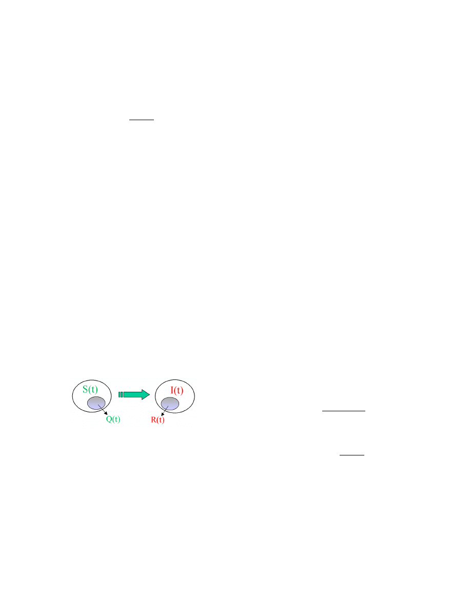
Figure 1: Interactions between infectious and sus-
ceptible hosts

The simple epidemic model (1) is derived based on the

interactions between infectious hosts and susceptible hosts.
Before we implement dynamic quarantine, a worm propa-
gates according to simple epidemic model (1) with the pair-
wise rate of infection β. When we implement dynamic quar-
antine on the system, Fig. 1 shows that the interactions
now are between [I(t) − R(t)] and [S(t) − Q(t)]. Therefore,
a worm’s propagation under dynamic quarantine follows

dI(t)/dt = β[I(t) − R(t)][S(t) − Q(t)]

= β

I(t)[N − I(t)]

(12)

where

β

= (1

− p

1

)(1

− p

2

)β

(13)

is the effective pairwise rate of infection.

Equation (12) shows that under dynamic quarantine, a

worm still propagates according to simple epidemic model
but with slower spreading speed. The dynamic quarantine
decreases a worm’s pairwise rate of infection β by the fac-
tor of (1

− p

1

)(1

− p

2

): the larger the effective quarantine

probabilities p

1

and p

2

are, the slower the worm can prop-

agate. Therefore, when we implement the dynamic quaran-
tine, it can provide us precious time to take counteractions
— patching vulnerable computers and cleaning infected ones
— before a worm infects the major part of a network.

4.2

Worm Modeling Based on Kermack
-Mckendrick Epidemic Model

Next, we analyze the impact of dynamic quarantine on

a worm’s propagation based on the Kermack-Mckendrick
epidemic model, i.e., we consider the removal process of
infectious hosts. As in the Kermack-Mckendrick epidemic
model, U (t) is the number of removed hosts from infectious
and it follows dU (t)/dt = γI(t) as shown in (3). For the
dynamic quarantine system, we assume that we remove in-
fectious hosts uniformly from I(t), regardless of whether a
removed host is under quarantine or not when we remove it.

Before we consider removal process, R(t) = p

1

I(t) and

Q(t) = p

2

S(t). When we consider removal process of infec-

tious hosts, since it has nothing to do with susceptible hosts,
Q(t) = p

2

S(t) still holds. However, Equation (5) should be

modified to consider the removed hosts from R(t) during
the time (t − T ) to t. Since the removal process uniformly
removes infectious hosts from I(t), the removal rate from
quarantined R(t) should be γR(t) at time t. Therefore, we
can extend (5) to derive

R(t) =

t

t−T

[I(τ ) − R(τ )]λ

1

dτ −

t

t−T

γR(τ )dτ.

(14)

With the same assumption that R(τ ) R(t) and I(τ )

I(t), ∀τ ∈ [t − T, t], from (14) we can derive

R(t) = q

1

I(t),

(15)

where

q

1

=

λ

1

T

1 + (λ

1

+ γ)T

(16)

is the effective quarantine probability of infectious hosts for a
worm’s propagation with removal process. For consistence,
we denote

q

2

= p

2

=

λ

2

T

1 + λ

2

T

(17)

as the effective quarantine probability of susceptible hosts
for a worm’s propagation with removal process, i.e.,

Q(t) = q

2

S(t).

(18)

A worm’s propagation follows

dI(t)/dt = β[I(t) − R(t)][S(t) − Q(t)] − γI(t)

= β

I(t)S(t) − γI(t)

(19)

where

β

= (1

− q

1

)(1

− q

2

)β

(20)

is the effective pairwise rate of infection for a worm’s prop-
agation with removal process.

The worm propagation model (19) is the same as the

Kermack-Mckendrick model (3), except that the pairwise
rate of infection β

is decreased from β by the factor of

(1

− q

1

)(1

− q

2

). The new dynamic quarantine system will

have an epidemic threshold ρ

that is

ρ

≡ γ/β

=

1

(1

− q

1

)(1

− q

2

)

ρ.

(21)

ρ

is increased from the original value ρ by the factor of

1

(1−q

1

)(1−q

2

)

. If the initial number of susceptible hosts S(0)

has the relationship S(0) > ρ and S(0) < ρ

, then according

to the Kermack-Mckendrick epidemic threshold theorem, a
worm will spread out in the original system but will not be
able to spread out when we implement dynamic quarantine
on the system.

In other words, the dynamic quarantine

method reduces the chance for a worm to form an outbreak.

4.3

Worm Modeling by Considering the Clean-
ing of Quarantined Infectious Hosts

In the previous model (19), all infectious hosts have an

equal probability to be removed. However, a more realistic
scenario is that security staffs only inspect the hosts that
have raised alarm and have been quarantined. The reasons
are: first, the limited human resources do not permit the
full-scale inspection of all hosts; second, alarmed hosts are
more likely to be infected by a worm. Therefore, in such
a dynamic quarantine system, only infectious hosts in the
quarantined population R(t) could be removed.

In this case, the number of removed hosts U (t) (from

quarantined infectious hosts R(t)) follows dU (t)/dt = γR(t).
The formula (14) is still correct for this situation. Now the
worm propagation model is

dI(t)/dt = β[I(t) − R(t)][S(t) − Q(t)] − γR(t)

= β

I(t)S(t) − γ

I(t)

(22)

where

γ

= q

1

γ

(23)

is the effective removal rate for this system.

We can see that the model (22) has the same format as the

Kermack-Mckendrick model (3). Therefore, all theorems of
the Kermack-Mckendrick model are valid here. Define the
epidemic threshold ρ

as

ρ

≡ γ

/β

=

q

1

(1

− q

1

)(1

− q

2

)

· γ

β

(24)

The epidemic threshold theorem states that if S(0) < ρ

, a

worm will not form an outbreak in this dynamic quarantine
system.

Note that all our analysis formulas are based on two as-

sumptions: first, the quarantine time T is small such that






R(τ ) R(t)
I(τ )

I(t)

S(τ )

S(t)

∀τ ∈ [t − T, t];

(25)

second, Equation (5) and (14) rely on the law of large num-
ber since these two equations use the mean values of λ

1

and λ

2

without considering stochastic effects — these two

equations are accurate only when I(t) − R(t) is large (the
formula of Q(t) is correct only when S(t) − Q(t) is large). In
the next section, we will use simulations to demonstrate how
these two assumptions affect the accuracy of our analysis.

5.

SIMULATION EXPERIMENTS

5.1

Simulation Settings

Worm propagation is a discrete-event dynamic system;

event-driven simulation is the most accurate method to sim-
ulate the propagation of a worm. However, we are interested
in the propagation of a worm in a large network system — an
event-driven simulation will be too time-consuming. There-
fore, we use discrete-time simulation in this paper.

We try to simulate a worm similar to the Slammer worm

on January 25th, 2003. According to [12], Slammer sent out
on average 4,000 scans per host per second at the worm’s
early growth phase. From their monitors, the authors in
[12] observed about 75,000 infected hosts in the first 30 min-
utes. Therefore, in our simulation, we assume that the vul-
nerable population is N = 75, 000 and the worm’s average
scan rate is η = 4000 per second. The authors in [19] pro-
vide a formula to estimate the size of vulnerable population
from a worm’s scan rate and infection rate.

We can re-

versely use that formula to derive the worm’s infection rate
α = ηN/2

32

= 0.0698, i.e., an infected host can probe on

average 0.0698 hosts among those 75,000 initially vulnerable
ones. We also assume I(0) = 10, i.e., 10 vulnerable hosts in
the system are infectious at the beginning.

To increase the accuracy of our discrete-time simulation,

we use 0.05 second as the discrete time unit, i.e., the simu-
lation program will iterate 20 times for simulating 1 second
of a worm’s propagation.

When we consider the dynamic quarantine, we assume

that the time before a host is alarmed follows exponen-
tial distribution: the quarantine rate of infectious hosts is
λ

1

= 0.2 per second, i.e., on average an infectious host can

propagate for about 5 seconds before it is alarmed and quar-
antined; the quarantine rate of susceptible hosts is λ

2

=

0.00002315 per second, i.e., the worm anomaly detection
program will give on average twice false alarms for a healthy
host per day. We set the quarantine time to be T = 10 sec-
onds.

5.2

Worm Propagation without Considering
Removal Process

We first consider a worm’s propagation without removal

of infectious hosts. In this case, in the original system where
there is no dynamic quarantine, a worm will propagate ac-
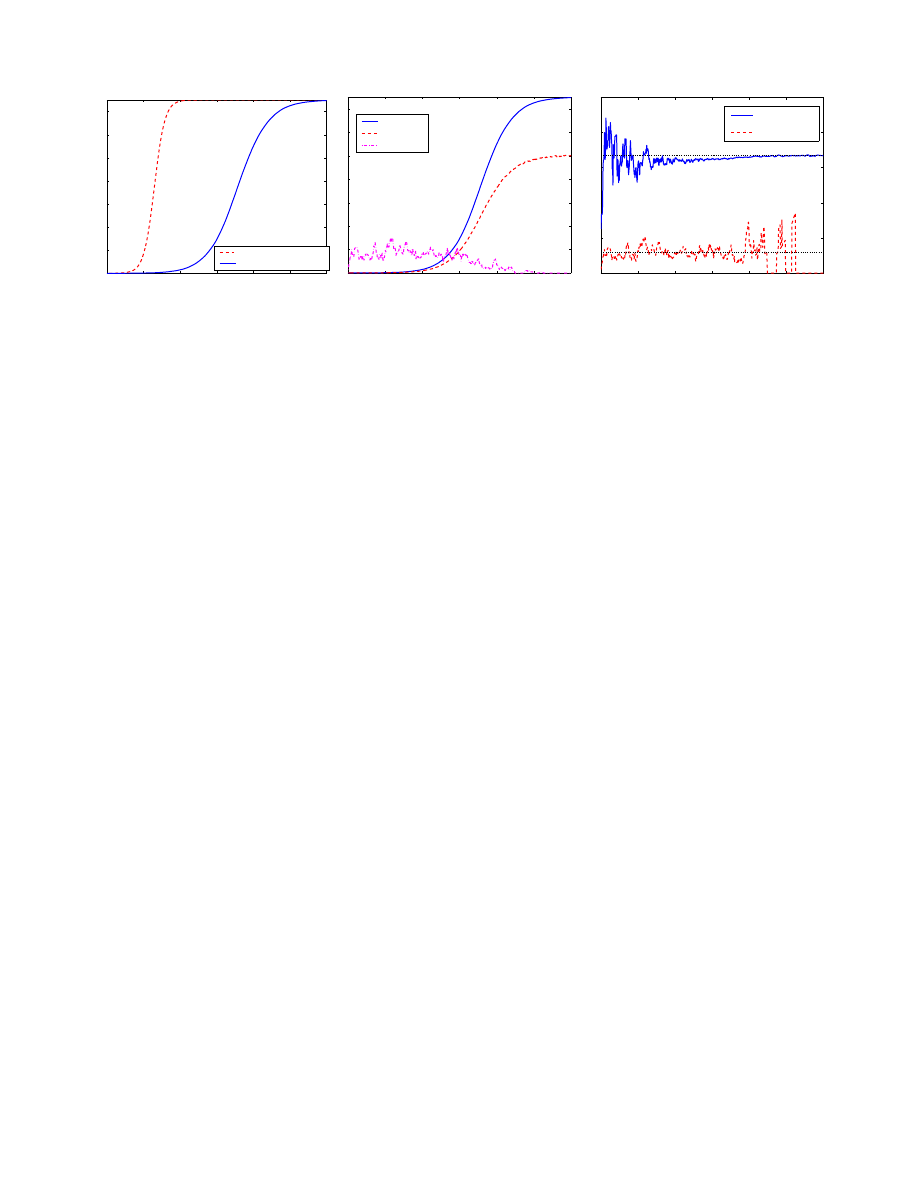
cording to the simple epidemic model (1). Fig. 2(a) shows
the number of infectious hosts I(t) as a function of time t
when a worm propagates in the dynamic quarantine system.
It compares the worm’s propagation in the dynamic quar-
antine system with the worm’s propagation in the original
system. This figure shows that in the dynamic quarantine
system, a worm still propagates according to the epidemic
model (1), but propagates at a much slower speed.

Fig. 2(b) shows the dynamics of I(t), R(t) and Q(t) as

functions of time t. Because λ

2

is very small, the number

of quarantined susceptible hosts, Q(t), is much smaller than
I(t) and R(t). Thus we enlarge Q(t) by 500 times in order
to show I(t), R(t), and Q(t) in the same figure. This figure

0

100

200

300

400

500

600

0

1

2

3

4

5

6

7

x 10

4

Time t (second)

I(t)

Original system
Quarantine system

a. Worm propagation comparison

0

100

200

300

400

500

600

0

1

2

3

4

5

6

7

x 10

4

Time t (second)

I(t)
R(t)
500

⋅

Q(t)

b. Worm propagation under

dynamic quarantine

0

100

200

300

400

500

600

0

0.2

0.4

0.6

0.8

1

Time t (second)

p’

1

500

⋅ p’

2

c. Observed effective quarantine

probabilities

Figure 2: Worm propagation without considering removal process (one simulation run)
N = 75, 000, α = 0.0698, T = 10, λ

1

= 0.2, λ

2

= 0.00002315

shows that the random effect of a worm’s propagation shows
up in the small value of Q(t); but because of the law of large
number, the curves of I(t) and R(t) are smooth.

In order to verify the formulas of R(t) and Q(t) in (8)

and (10), we calculate the ratio of R(t)/I(t) and Q(t)/S(t)
from the simulation at each second t = 1, 2, · · · . We plot
these two ratios as functions of time t in Fig. 2(c) compared
with their theoretical values from (9) and (11). Because the
value of p

2

is very small, we enlarge it 500 times in order to

show p

1

and p

2

in the same figure. This figure shows that

the formulas (9) and (11) are accurate for most part of a
worm’s propagation. Even when the assumption (25) is not
accurate during the worm’s fast spreading period (from 250
seconds to 400 seconds when R(t) and I(t) increase quickly),
the formulas (9) and (11) still hold.

Fig. 2(c) shows that the formula (9) of p

1

is not accurate

at the beginning of a worm’s propagation. This is because
the formula (9) relies on the law of large number: at the
beginning when I(t) is small, it is not accurate to directly
use the mean value λ

1

to calculate p

1

.

This is also the

reason of the large oscillation of p

2

at the end of a worm’s

propagation when S(t) is small. In the whole process of a
worm’s propagation, the large oscillation of p

2

is due to the

small and variable Q(t) as shown in Fig. 2(b).

5.2.1

Variability in Worm Propagation

Worm propagation is in fact a stochastic process. A small

random variations at the beginning of a worm’s growth can
affect dramatically how quickly the worm spreads [11]. Here
we conduct experiments to check how the variability in a
worm’s propagation affects our analysis.

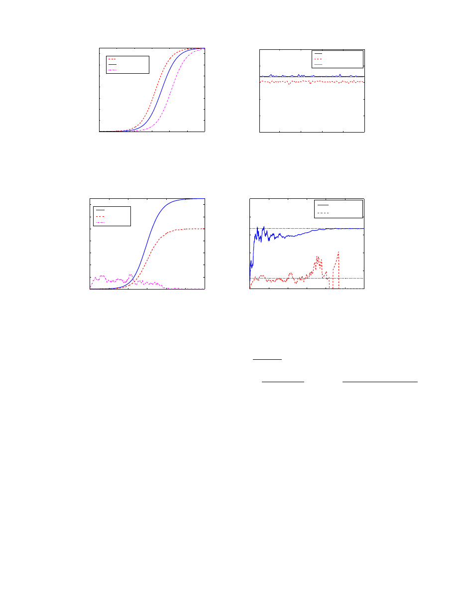
With the same

simulation parameters above, we run the simulations for 100
times. Fig. 3(a) shows the upper and lower bounds and the
average value of the number of infectious hosts in these 100
simulation runs.

For each of these 100 simulation runs, we calculate the

ratio p

1

= R(t)/I(t) after the worm infects 1% of the popu-

lation (the worm in different simulation runs will take differ-
ent lengths of time to infect 1% hosts). Then we obtain the
maximum and minimum values of the observed p

1

for each

simulation run — the oscillation of the observed p

1

will not

exceed this boundary after the worm infects 1% population.
We plot this boundary in Fig. 3(b) for each of these 100 sim-

ulation runs. In order to check if the formula of p

1

becomes

less accurate when a worm propagates faster, in Fig. 3(b)
we have sorted these 100 simulation runs according to the
time when the worm infects 1% population. In other words,
the worm in simulation i infects 1% of vulnerable hosts ear-
lier than the worm in simulation j does if i < j. This figure
shows that the accuracy of our analysis does not depend on
how a worm propagates in different situations — if a worm
propagates faster, i.e., I(t) increases faster, then the number
of quarantined infectious hosts R(t) will also increase faster
accordingly.

5.2.2

Effect of a Large Quarantine Time

T

The simulation in Fig. 2 shows that our analysis is robust

to the assumption in (25). Then what happens if we select
a larger quarantine time T ? To answer this, we run another
simulation with T = 30 seconds and show the simulation
results in Fig. 4. In this simulation, we try to let a worm to
propagate in the similar speed as the one shown in Fig. 2;
thus we choose λ

1

= 0.2/3 and λ

2

= 0.00002315/3 in order

to let p

1

and p

2

in this simulation to have the same values

as in the simulation in Fig. 2. All other parameters are the
same as what used in that simulation.

According to our analysis, in this simulation a worm should

propagate with the same speed as the one shown in Fig.
2(b). However, Fig. 4(a) shows that in this simulation, the
worm propagates a little bit faster. This is because the as-
sumption (25) in our analysis is not accurate anymore for
this simulation. During the fast increasing part of I(t) and
R(t) (before time 350 seconds), I(t) and R(t) will have

R(τ ) < R(t)
I(τ )

< I(t)

∀τ ∈ [t − T, t];

(26)

thus (7) will become R(t) < [I(t) − R(t)]λ

1

T . In this case,

the relationship between R(t) and I(t) is

R(t) < p

1

I(t)

(27)

instead of the formula (8). Fig. 4(b) verifies this analysis —
the observed p

1

is smaller than the theoretical value from (9)

before time 350. Since the number of quarantined infectious
hosts is smaller than the one in the simulation shown in

0

100

200

300

400

500

600

0

1

2

3

4

5

6

7

x 10

4

Time t (second)

I(t)

Upper bound
Mean value
Lower bound

a. Variability in worm propagation

20

40

60

80

100

0

0.2

0.4

0.6

0.8

1

100 simulation runs (sorted)

p’

1

Upper bound
Lower bound
Theoretical value

b. Bounds of p

1

after the worm infects

1% population

Figure 3: Variability effect in worm propagation (100 simulation runs)
N = 75, 000, α = 0.0698, T = 10, λ

1

= 0.2, λ

2

= 0.00002315

0

100

200

300

400

500

600

0

1

2

3

4

5

6

7

x 10

4

Time t (second)

I(t)
R(t)
500

⋅

Q(t)

a. Worm propagation under

dynamic quarantine

0

100

200

300

400

500

600

0

0.2

0.4

0.6

0.8

1

Time t (second)

p’

1

500

⋅ p’

2

b. Effective quarantine probabilities

Figure 4: Worm propagation with a large quarantine time
N = 75, 000, α = 0.0698, T = 30, λ

1

= 0.2/3, λ

2

= 0.00002315/3

Fig. 2(b), there are more non-quarantine infectious hosts
trying to infect others in this simulation. Therefore, worm
propagation in this simulation is faster.

5.3

Worm Propagation Considering Removal
Process

5.3.1

Quarantine System Described by Model (19)

Now we study a worm’s propagation when we consider

the removal of infectious hosts. First, we consider the dy-
namic quarantine system described by the model (19), i.e.,
all infectious hosts have the equal probability to be removed
regardless whether they are quarantined or not.

We briefly explain how we choose the removal rate γ. To

study a worm’s propagation, we need to let the worm to
spread out, which means we should select parameters such
that S(0) > ρ

according to the epidemic threshold theorem.

Since S(0) = N − I(0) ≈ N , from (2), (4), and (21), we
should select γ to satisfy

γ < (1 − q

1

)(1

− q

2

)α < α

(28)

Thus α is an upper bound for γ. From (16), we know that

q

1

>

λ

1

T

1+(λ

1

+α)T

. Thus a tighter upper bound for γ is

γ < (1−

λ

1

T

1 + (λ

1

+ α)T

)(1

−q

2

)α =

(1 + αT )α

(1 + λ

2

T )[1 + (λ

1

+ α)T ]

(29)

In this simulation, we use the same parameters as what

used in the simulation shown in Fig. 2. In this case, Equa-
tion (29) shows that we should choose γ < 0.032. Therefore,
we choose γ = 0.01 in the simulation.

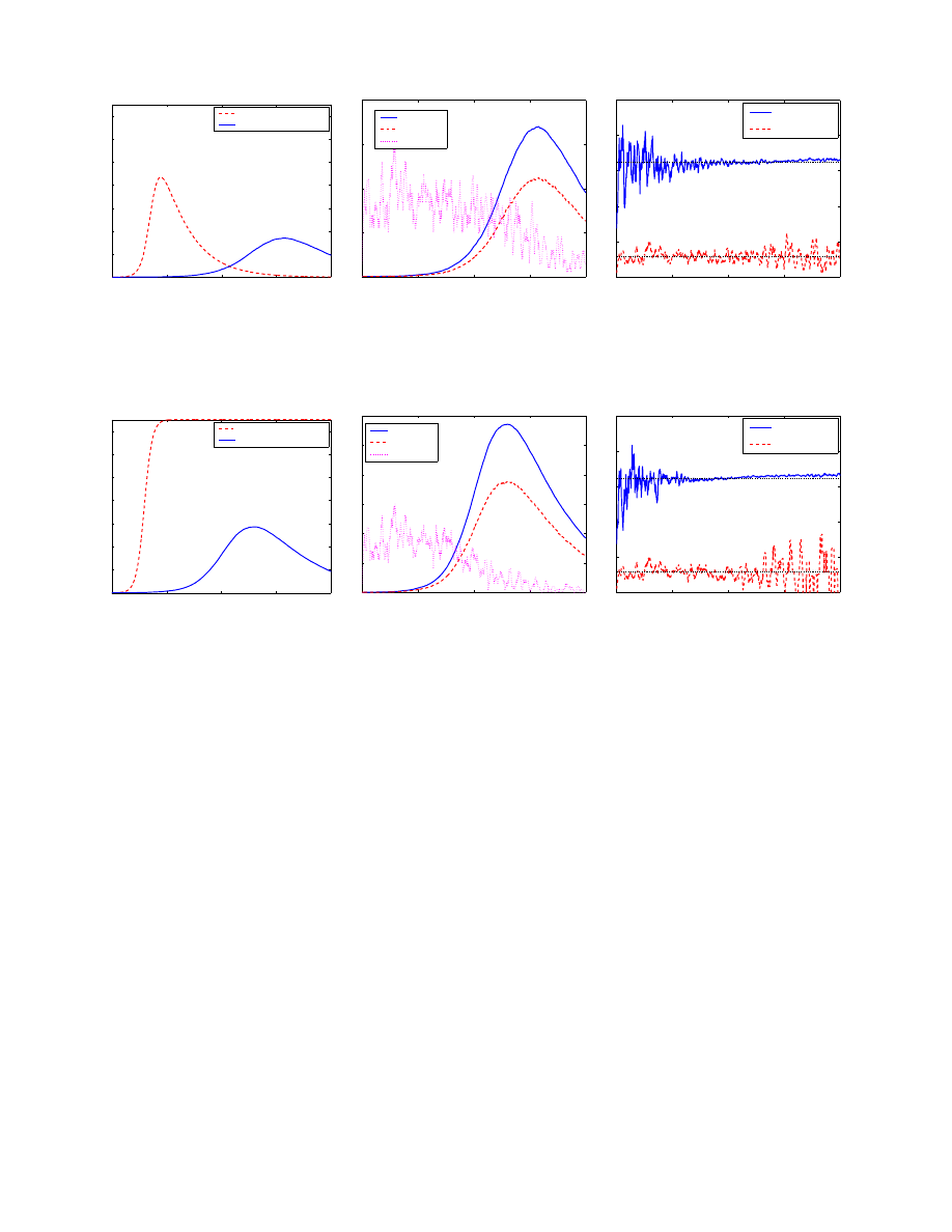
The simulation results are shown in Fig. 5; this figure has

the same format and meanings as Fig. 2. The “original sys-
tem” in Fig. 5(a) is the non-quarantine system described by
the Kermack-Mckendrick model (3). Note that the Y-axis
scales in Fig. 5(a)(b) are different. Fig. 5 shows that our
analysis and the model (19) are correct: in a dynamic quar-
antine system with the removal process, a worm propagates
according to the model (19) with much slower propagation
speed than the worm does in the original system without
dynamic quarantine defense.

5.3.2

Quarantine System Described by Model (22)

Next we consider the dynamic quarantine system described

by the model (22), i.e., only quarantined infectious hosts are

0

200

400

600

800

0

1

2

3

4

5

6

7

x 10

4

Time t (second)

I(t)

Original system
Quarantine system

a. Worm propagation comparison

0

200

400

600

800

0

0.5

1

1.5

2

x 10

4

Time t (second)

I(t)
R(t)
500

⋅

Q(t)

b. Worm propagation under

dynamic quarantine

0

200

400

600

800

0

0.2

0.4

0.6

0.8

1

Time t (second)

q’

1

500

⋅ q’

2

c. Observed effective quarantine

probabilities

Figure 5: Worm propagation by considering removal process (from all infectious hosts)
N = 75, 000, α = 0.0698, T = 10, λ

1

= 0.2, λ

2

= 0.00002315, γ = 0.01

0

200

400

600

800

0

1

2

3

4

5

6

7

x 10

4

I(t)

Time t (second)

Original system
Quarantine system

a. Worm propagation comparison

0

200

400

600

800

0

0.5

1

1.5

2

2.5

3

x 10

4

Time t (second)

I(t)
R(t)
500

⋅

Q(t)

b. Worm propagation under

dynamic quarantine

0

200

400

600

800

0

0.2

0.4

0.6

0.8

1

Time t (second)

q’

1

500

⋅ q’

2

c. Observed effective quarantine

probabilities

Figure 6: Worm propagation by considering removal process (only from quarantined infectious hosts)
N = 75, 000, α = 0.0698, T = 10, λ

1

= 0.2, λ

2

= 0.00002315, γ = 0.01

possible to be removed. The simulation results are shown in
Fig. 6, which has the same format and meanings as Fig. 5.
The “original system” in Fig. 6(a) is the non-quarantine sys-
tem without removal process, i.e., a worm’s propagation in
this system can be described by the simple epidemic model
(1). Fig. 6 shows that our analysis and the model (22)
are correct; in such a dynamic quarantine system, a worm
propagates much slower and follows the model (22).

6.

CONCLUSION

Enlightened by the methods used in epidemic disease con-

trol in the real world, we present a dynamic quarantine
method based on the principle “assume guilty before proven
innocent”.

We quarantine a host whenever its behavior

looks suspicious by blocking traffic on the anomaly port,
then we will release the quarantine after a short time, even
if the host has not been inspected by security staffs yet. As
a first step, in this paper we analyze the dynamic quaran-
tine system that has constant quarantine time and worm
detection threshold. Our mathematical analysis shows that
in the dynamic quarantine system, a worm still propagates
according to traditional epidemic models, but with slower
propagation speed and higher epidemic threshold.

To derive simple mathematical formulas, in this paper we

have simplified the quarantine system and the dynamics of a
worm’s propagation. For example, we have assumed that all
hosts in the system have the same quarantine rates λ

1

and

λ

2

. We need to further study the case where each host has

different quarantine rates. In order to use classical epidemic
models, we also have assumed that the system is homoge-
neous and the contact rate is constant for all hosts at any
time. We need to study how to extend the analysis in this
paper to a non-homogeneous system with variable contact
rate.

A more advanced dynamic quarantine system should have

dynamically changing quarantine time and detection thresh-
old during a worm’s propagation. Like what people act in
epidemic disease control in the real world, if a worm is more
infectious and poses more damage to our networks, the dy-
namic quarantine defense should be more aggressive — the
anomaly detection should be more sensitive to the worm’s
activities, and the quarantine time should become longer to
further constrain quarantined infectious hosts. Our long-
term objective is to develop a “feedback control dynamic
quarantine system”. This feedback quarantine system can
optimally adjust the anomaly detection threshold and the
quarantine time in order to minimize the cost of false alarms

and at the same time to slow down a worm’s spreading speed
as much as possible. This paper is our first step into that
direction.

7.

ACKNOWLEDGEMENTS

This work is supported in part by ARO contract DAAD19-

01-1-0610; by DARPA under Contract DOD F30602-00-0554;
by NSF under grant EIA-0080119, ANI9980552, ANI-0208116,
and by Air Force Research Lab.

8.

REFERENCES

[1] Z. Chen, L. Gao, and K. Kwiat. Modeling the Spread

of Active Worms. IEEE INFOCOM, 2003.

[2] D.J. Daley and J. Gani. Epidemic Modelling: An

Introduction. Cambridge University Press, 1999.

[3] J. O. Kephart and S. R. White. Directed-graph

Epidemiological Models of Computer Viruses. In
Proceedings of the IEEE Symposimum on Security and
Privacy, 1991.

[4] J. O. Kephart, D. M. Chess, and S. R. White.

Computers and Epidemiology. IEEE Spectrum, 1993.

[5] J. O. Kephart and S. R. White. Measuring and

Modeling Computer Virus Prevalence. In Proceedings
of the IEEE Symposimum on Security and Privacy,
1993.

[6] O. Kreidl and T. Frazier. Feedback Control Applied to

Survivability: a Host-Based Autonomic Defense
System, IEEE Transactions on Reliability, Vol. 52,
No. 3, 2003.

[7] T. Liston. Welcome to My Tarpit: The Tactical and

Strategic Use of LaBrea. Dshield.org White paper,
2001.
http://hts.dshield.org/LaBrea/LaBrea.txt

[8] P. Lindstrom. Guide to Intrusion Prevention.

Information Security Magazine, October, 2002.

[9] D. Seeley. A tour of the worm. In Proceedings of the

Winter Usenix Conference, San Diego, CA, 1989.

[10] D. Moore, C. Shannon, and J. Brown. Code-Red: a

case study on the spread and victims of an Internet
Worm. In Proc. ACM/USENIX Internet Measurement
Workshop, France, November, 2002.

[11] D. Moore, C. Shannon, G. M. Voelker, and S. Savage.

Internet Quarantine: Requirements for Containing
Self-Propagating Code. In IEEE INFOCOM, 2003.

[12] D. Moore, V. Paxson, S. Savage, C. Shannon, S.

Staniford, and N. Weaver. Inside the Slammer Worm.
IEEE Security and Privacy, 1(4):33-39, July 2003.

[13] CAIDA. Dynamic Graphs of the Nimda worm.

http://www.caida.org/dynamic/analysis/security/nimda/

[14] S. Staniford, V. Paxson, and N. Weaver. How to Own

the Internet in Your Spare Time. In 11th Usenix
Security Symposium, San Francisco, August, 2002.

[15] Worm containment in the internal network. Silicon

Defense technical white paper, March, 2003.

[16] USA Today. The cost of ’Code Red’: $1.2 billion.

http://usatoday.com/tech/news/2001-08-01-code-red-
costs.htm

[17] M. Williamson. Throttling Viruses: Restricting

Propagation to Defeat Malicious Mobile Code. HP
Laboratories Technical Report, HPL-2002-172, 2002.

[18] C.C. Zou, W. Gong, and D. Towsley. Code Red Worm

Propagation Modeling and Analysis. In 9th ACM
Symposium on Computer and Communication
Security, pages 138-147, Washington DC, 2002.

[19] C.C. Zou, L. Gao, W. Gong, and D. Towsley.

Monitoring and Early Warning for Internet Worms. In
10th ACM Symposium on Computer and
Communication Security, Washington DC, 2003.