Code Red Worm Propagation Modeling and Analysis

∗

Cliff Changchun Zou

Dept. Electrical &

Computer Engineering

Univ. Massachusetts

Amherst, MA

[e-mail]

Weibo Gong

Dept. Electrical &

Computer Engineering

Univ. Massachusetts

Amherst, MA

[e-mail]

Don Towsley

Dept. Computer Science

Univ. Massachusetts

Amherst, MA

[e-mail]

ABSTRACT

The Code Red worm incident of July 2001 has stimulated
activities to model and analyze Internet worm propagation.
In this paper we provide a careful analysis of Code Red prop-
agation by accounting for two factors: one is the dynamic
countermeasures taken by ISPs and users; the other is the
slowed down worm infection rate because Code Red rampant
propagation caused congestion and troubles to some routers.
Based on the classical epidemic Kermack-Mckendrick model,
we derive a general Internet worm model called the two-
factor worm model.

Simulations and numerical solutions

of the two-factor worm model match the observed data of
Code Red worm better than previous models do. This model
leads to a better understanding and prediction of the scale
and speed of Internet worm spreading.

Categories and Subject Descriptors

H.1 [Models and Principles]: Miscellaneous

General Terms

Security, Human Factors

Keywords

Internet worm modeling, epidemic model, two-factor worm
model

1.

INTRODUCTION

The easy access and wide usage of the Internet makes

it a primary target for malicious activities. In particular,

∗

This work was supported in part by ARO contract

DAAD19-01-1-0610; by contract 2000-DT-CX-K001 from
the U.S. Department of Justice, Office of Justice Programs;
by DARPA under contract F30602-00-2-0554 and by NSF
under Grant EIA-0080119.

Permission to make digital or hard copies of all or part of this work for
personal or classroom use is granted without fee provided that copies are
not made or distributed for profit or commercial advantage and that copies
bear this notice and the full citation on the first page. To copy otherwise, to
republish, to post on servers or to redistribute to lists, requires prior specific
permission and/or a fee.
CCS’02, November 18-22, 2002, Washington, DC, USA.
Copyright 2002 ACM 1-58113-612-9/02/0011 ...

$

5.00.

the Internet has become a powerful mechanism for propa-
gating malicious software programs. Worms, defined as au-
tonomous programs that spread through computer networks
by searching, attacking, and infecting remote computers au-
tomatically, have been developed for more than 10 years
since the first Morris worm [30]. Today, our computing in-
frastructure is more vulnerable than ever before [28]. The
Code Red worm and Nimda worm incidents of 2001 have
shown us how vulnerable our networks are and how fast
a virulent worm can spread; furthermore, Weaver presented
some design principles for worms such that they could spread
even faster [34]. In order to defend against future worms, we
need to understand various properties of worms: the prop-
agation pattern during the lifetime of worms; the impact of
patching, awareness and other human countermeasures; the
impact of network traffic, network topology, etc.

An accurate Internet worm model provides insight into

worm behavior. It aids in identifying the weakness in the
worm spreading chain and provides accurate prediction for
the purpose of damage assessment for a new worm threat. In
epidemiology research, there exist several deterministic and
stochastic models for virus spreading [1, 2, 3, 15]; however,
few models exist for Internet worm propagation modeling.
Kephart, White and Chess of IBM performed a series of
studies from 1991 to 1993 on viral infection based on epi-
demiology models [20, 21, 22]. Traditional epidemic models
are all homogeneous, in the sense that an infected host is
equally likely to infect any of other susceptible hosts [3, 15].
Considering the local interactions of viruses at that time,
[20, 21] extended those epidemic models onto some non-
homogeneous networks: random graph, two-dimensional lat-
tice and tree-like hierarchical graph. Though at that time
the local interaction assumption was accurate because of
sharing disks, today it’s no longer valid for worm modeling
when most worms propagate through the Internet and are
able to directly hit a target. In addition, the authors used
susceptible - infected - susceptible (SIS) model for viruses
modeling, which assumes that a cured computer can be re-
infected immediately. However, SIS model is not suitable
for modeling a single worm propagation since once an in-
fected computer is patched or cleaned, it’s more likely to
be immune to this worm. Wang et al. presented simula-
tion results of a simple virus propagation on clustered and
tree-like hierarchical networks [32]. They showed that in
certain topologies selective immunization can significantly
slow down virus propagation [32]. However, their conclu-
sion was based on a tree-like hierarchic topology, which is
not suitable for the Internet.

The Code Red worm incident of July 2001 has stimulated

activities to model and analyze Internet worm propagation.
Staniford et al. used the classical simple epidemic equa-
tion to model Code Red spread right after the July 19th
incident [31]. Their model matched pretty well with the
limited observed data. Heberlein presented a visual simula-
tion of Code Red worm propagation on Incident.com [17].
Moore provided some valuable observed data and a detailed
analysis of Code Red worm behavior [27]. Weaver provided
some worm design principles, which can be used to pro-
duce worms that spread even faster than the Code Red and
Nimda worms [34].

Previous work on worm modeling neglects the dynamic

effect of human countermeasures on worm behavior. Wang
et al. [32] investigated the immunization defense. But they
considered only static immunization, which means that a
fraction of the hosts are immunized before the worm prop-
agates. In reality, human countermeasures are dynamic ac-
tions and play a major role in slowing down worm propa-
gation and preventing worm outbreaks. Many new viruses
and worms come out every day. Most of them, however,
die away without infecting many computers due to human
countermeasures.

Human countermeasures against a virus or worm include:

• Using anti-virus softwares or special programs to clean

infected computers.

• Patching or upgrading susceptible computers to make

them immune to the virus or worm.

• Setting up filters on firewalls or routers to filter or

block the virus or worm traffic.

• Disconnecting networks or computers when no effec-

tive methods are available.

In the epidemic modeling area, the virus infection rate is

assumed to be constant. Previous Internet virus and worm
models (except [34]) treat the time required for an infected
host to find a target, whether it is already infected or still
susceptible, as constant as well. In [34], the author treated
the infection rate as a random variable by considering the
unsuccessful IP scan attempts of a worm. The mean value
of the infection rate, however, is still assumed to be constant
over time. A constant infection rate is reasonable for model-
ing epidemics but may not be valid for Internet viruses and
worms.

In this paper, through analysis of the Code Red incident of

July 19th 2001, we find that there were two factors affecting
Code Red propagation: one is the dynamic countermeasures
taken by ISPs and users; the other is the slowed down worm
infection rate because the rampant propagation of Code Red
caused congestion and troubles to some routers. By account-
ing for both the dynamic aspects of human countermeasures
and the variable infection rate, we derive a more accurate
worm propagation model: the two-factor worm model. Sim-
ulation results and numerical solutions show that our model
matches well with the observed Code Red data. In partic-
ular, it explains the decrease in Code Red scan attempts
observed during the last several hours of July 19th [13, 16]
before Code Red ceased propagation — none of previous
worm models are able to explain such phenomenon. It also
shows that Code Red didn’t infect almost all susceptible on-
line computers at 19:00 UTC as concluded in [31]. Instead,

Code Red infected roughly 60% of all susceptible online com-
puters at that time.

The rest of the paper is organized as follows. Section 2

gives a brief description of the Code Red worm incident of
July 2001. In Section 3, we give a brief review of two clas-
sical epidemic models and point out several problems that
they exhibit when modeling Internet worms. In Section 4,
we describe the two factors that are unique to the Internet
worm propagation and present a new Internet worm model:
the two-factor worm model. We present Code Red simula-
tions based on the new model in Section 5. We derive a set
of differential equations describing the behavior of the two-
factor worm model in Section 6 and provide corresponding
numerical solutions. Both the simulation results and the
numerical solutions match well with the observed Code Red
data. Section 7 concludes the paper with some discussions.

2.

BACKGROUND ON CODE RED WORM

On June 18th 2001 a serious Windows IIS vulnerabil-

ity was discovered [24]. After almost one month, the first
version of Code Red worm that exploited this vulnerabil-
ity emerged on July 13th, 2001 [11]. Due to a code error
in its random number generator, it did not propagate well
[23]. The truly virulent strain of the worm (Code Red ver-
sion 2) began to spread around 10:00 UTC of July 19th
[27]. This new worm had implemented the correct random
number generator. It generated 100 threads. Each of the
first 99 threads randomly chose one IP address and tried to
set up connection on port 80 with the target machine [11]
(If the system was an English Windows 2000 system, the
100th worm thread would deface the infected system’s web
site, otherwise the thread was used to infect other systems,
too). If the connection was successful, the worm would send
a copy of itself to the victim web server to compromise it
and continue to find another web server. If the victim was
not a web server or the connection could not be setup, the
worm thread would randomly generate another IP address
to probe. The timeout of the Code Red connection request
was programmed to be 21 seconds [29]. Code Red can ex-
ploit only Windows 2000 with IIS server installed — it can’t
infect Windows NT because the jump address in the code is
invalid under NT [12].

Code Red worm (version 2) was programmed to uniformly

scan the IP address space. Netcraft web server survey showed
that there were about 6 million Windows IIS web servers at
the end of June 2001[19]. If we conservatively assume that
there were less than 2 million IIS servers online on July 19th,
on average each worm would need to perform more than
2000 IP scans before it could find a Windows IIS server.
The worm would need, on average, more than 4000 IP scans
to find a target if the number of Windows IIS servers on-
line was less than 1 million. Code Red worm continued to
spread on July 19th until 0:00 UTC July 20th, after which
the worm stopped propagation by design [4].

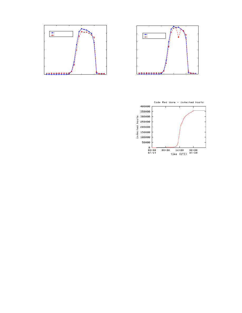
Three independent observed data sets are available on the

Code Red incident of July 19th. Goldsmith and Eichman
collected two types of data on two class B networks indepen-
dently [13, 16]: one is the number of Code Red worm port
80 scans during each hour, the other is the number of unique
sources that generated these scans during each hour. The
number of Code Red scan attempts from these two data sets
are plotted in Fig. 1(a) and the number of unique sources
in Fig. 1(b) as functions of time.

04:00

09:00

14:00

19:00

00:00

04:00

0

1

2

3

4

5

6

x 10

5

UTC hours (July 19 − 20)

scan attempt number

Code Red scan attempts per hour on 2 Class B networks

Dave Goldsmith
Ken Eichman

a. Code Red scan attempts

04:00

09:00

14:00

19:00

00:00

04:00

0

2

4

6

8

10

12

x 10

4

UTC hours (July 19 − 20)

Unique source number

Code Red scan unique sources per hour on 2 Class B networks

Dave Goldsmith
Ken Eichman

b. Code Red scan unique sources

Figure 1: Code Red scan data on two Class B networks

Since Code Red worm was programmed to choose random

IP addresses to scan, each IP address is equally likely to be
scanned by a Code Red worm. It explains why the Code
Red probes on these two Class B networks were so similar
to each other as shown in Fig. 1.

Each of the two class B networks covers only 1/65536th of

the whole IP address space; therefore, the number of unique
sources and the number of scans in Fig. 1 are only a portion
of active Code Red worms on the whole Internet at that
time. However, they correctly exhibit the pattern of Code
Red propagation because of the uniform scan of Code Red
— this is the reason why we can use the data to study Code
Red propagation.

Because each infected computer would generate 99 simul-

taneous scans (one scan per thread) [11], the number of
worm scans was bigger than the number of unique sources.
However, Fig. 1 shows that the number of unique sources
and the number of scans have the identical evolvement over
time — both of them are able to represent Code Red propa-
gation on the Internet. For example, if the number of active
Code Red infected computers on the Internet increased 10
times in one hour, both the number of unique sources and
the number of scans observed by Goldsmith and Eichman
would increase about 10 times.

Moore et al. provided another valuable data set collected

on Code Red worm during the whole day of July 19th [27].
Not like the data collected by Goldsmith and Eichman, which
were recounted at each hour, Moore et al. recorded the time
of the first attempt of each infected host to spread the worm
to their networks. Thus the number of infected hosts in their
data is a non-decreasing function of time. The number of
infected hosts observed is shown in Fig. 2 as a function of
time t.

When rebooted, a Code Red infected computer went back

to susceptible state and could be reinfected again [4]. How-
ever, this would not affect the number of infected hosts
shown in Fig. 2 — a reinfected host would use the same
source IP to scan, thus it would not be recounted into the
data collected by Moore et al..

Moore et al. considered patching and filtering too when

they collected Code Red data [27]. The authors observed
that during the course of the day, many initially infected ma-
chines were patched, rebooted, or filtered and consequently
ceased to probe the Internet. A host that was previously

Figure 2: Observed Code Red propagation — num-
ber of infected hosts (from Caida.org)

infected was considered by the authors to be deactivated af-
ter no further unsolicited traffic was observed from it. The
number of observed deactivated hosts over time is shown in
Fig. 3.

Since Code Red worm was programmed to stop spreading

after 00:00 UTC July 20th, the number of infected hosts
stopped increasing after 00:00 UTC. Otherwise the curve
in Fig. 2 would have kept increasing to some extent. The
abrupt rise in host inactivity in Fig. 3 at 00:00 UTC is
also due to the worm design of stopping infection at the
midnight.

We are interested in the following issues: How can we ex-

plain these Code Red worm propagation curves shown in
Fig. 1, 2, and Fig. 3? What factors affect the spreading be-
havior of an Internet worm? Can we derive a more accurate
model for an Internet worm?

3.

USING EPIDEMIC MODELS TO MODEL
CODE RED WORM PROPAGATION

Computer viruses and worms are similar to biological viruses

on their self-replicating and propagation behaviors. Thus
the mathematical techniques which have been developed for
the study of biological infectious diseases might be adapted
to the study of computer viruses and worms propagation.

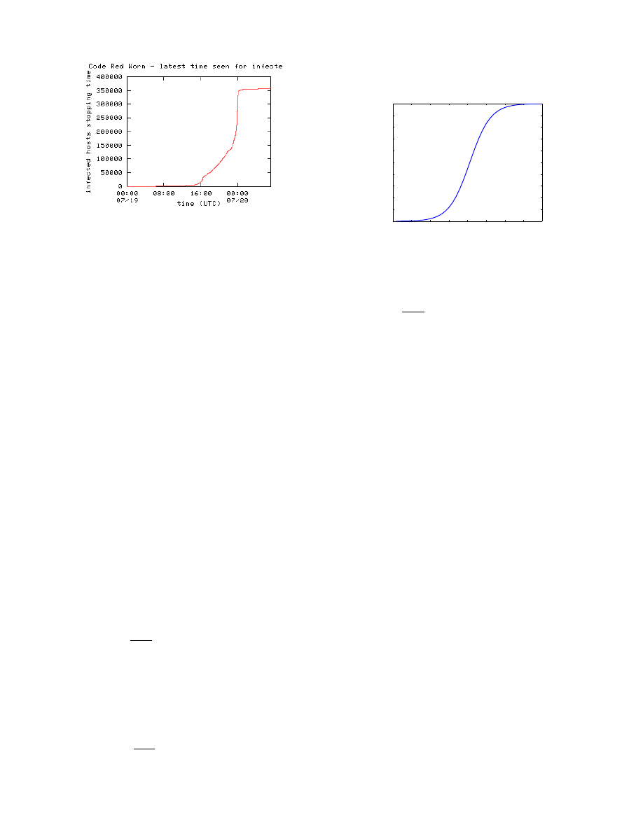
Figure 3: Observed Code Red propagation — num-
ber of deactivated hosts (from Caida.org)

In epidemiology area, both stochastic models and deter-

ministic models exist for modeling the spreading of infec-
tious diseases [1, 2, 3, 15]. Stochastic models are suitable
for small-scale system with simple virus dynamics; deter-
ministic models are suitable for large-scale system under the
assumption of mass action, relying on the law of large num-
ber [2]. When we model Internet worms propagation, we
consider a large-scale network with thousands to millions of
computers. Thus we will only consider and use determinis-
tic models in this paper. In this section, we introduce two
classical deterministic epidemic models, which are the bases
of our two-factor Internet worm model. We also point out
their problems when we try to use them to model Internet
worm propagation.

In epidemiology modeling, hosts that are vulnerable to

be infected by virus are called susceptible hosts; hosts that
have been infected and can infect others are called infectious
hosts; hosts that are immune or dead such that they can’t
be infected by virus are called removed hosts, no matter
whether they have been infected before or not. A host is
called an infected host at time t if it has been infected by
virus before t, no matter whether it is still infectious or is
removed [2] at time t. In this paper, we will use the same
terminology for computer worms modeling.

3.1

Classical simple epidemic model

In classical simple epidemic model, each host stays in one

of two states: susceptible or infectious. The model assumes
that once a host is infected by a virus, it will stay in infec-
tious state forever. Thus state transition of any host can
only be: susceptible

→ infectious [15]. The classical simple

epidemic model for a finite population is

dJ(t)

dt

= βJ(t)[N − J(t)],

(1)

where J(t) is the number of infected hosts at time t; N is the
size of population; and β is the infection rate. At beginning,
t = 0, J(0) hosts are infectious and the other N − J(0) hosts
are all susceptible.

Let a(t) = J(t)/N be the fraction of the population that

is infectious at time t . Dividing both sides of (1) by N

2

yields the equation used in [31]:

da(t)

dt

= ka(t)[1 − a(t)],

(2)

where k = βN . Using the same value k = 1.8 as what used
in [31], the dynamic curve of a(t) is plotted in Fig. 4.

0

5

10

15

20

25

30

35

40

0

0.1

0.2

0.3

0.4

0.5

0.6

0.7

0.8

0.9

1

Classical simple epidemic model

time: t

a(t)

Figure 4: Classical simple epidemic model (k = 1.8)

Let S(t) = N − J(t) denote the number of susceptible

hosts at time t. Replace J(t) in (1) by N − S(t) and we get

dS(t)

dt

=

−βS(t)[N − S(t)].

(3)

Equation (1) is identical with (3) except for a minus sign.

Thus the curve in Fig. 4 will remain the same when we
rotate it 180 degrees around the (t

half

, 0.5) point where

J(t

half

) = S(t

half

) = N/2. Fig. 4 and Eq. (2) show that

at the beginning when 1

− a(t) is roughly equal to 1, the

number of infectious hosts is nearly exponentially increased.
The propagation rate begins to decrease when about 80% of
all susceptible hosts have been infected.

Staniford et al. [31] presented a Code Red propagation

model based on the data provided by Eichman [18] up to
21:00 UTC July 19th. The model captures the key behavior
of the first half part of the Code Red dynamics. It is essen-
tially the classical simple epidemic model (1). We provide,
in this paper, a more detailed analysis that accounts for two
important factors involved in Code red spreading. Part of
our effort is to explain the evolution of Code Red spreading
after the beginning phase of its propagation. Although the
classical epidemic model can match the beginning phase of
Code Red spreading, it can’t explain the later part of Code
Red propagation: during the last five hours from 20:00 to
00:00 UTC, the worm scans kept decreasing (Fig. 1).

From the simple epidemic model (Fig. 4), the authors in

[31] concluded that Code Red came to saturating around
19:00 UTC — almost all susceptible IIS servers online on
July 19th had been infected around that time. The numer-
ical solution of our model in Section 6, however, shows that
only about 60% of all susceptible IIS servers online have
been infected around 19:00 UTC on July 19th.

3.2

Classical general epidemic model: Kermack-
Mckendrick model

In epidemiology area, Kermack-Mckendrick model consid-

ers the removal process of infectious hosts [15]. It assumes
that during an epidemic of a contagious disease, some infec-
tious hosts either recover or die; once a host recovers from
the disease, it will be immune to the disease forever — the
hosts are in “removed” state after they recover or die from
the disease. Thus each host stays in one of three states at
any time: susceptible, infectious, removed. Any host in the

system has either the state transition “susceptible

→ infec-

tious

→ removed” or stays in “susceptible” state forever.

Let I(t) denote the number of infectious hosts at time t.

We use R(t) to denote the number of removed hosts from
previously infectious hosts at time t. A removed host from
the infected population at time t is a host that is once in-
fected but has been disinfected or removed from circulation
before time t. Let J(t) denote the number of infected hosts
by time t, no matter whether they are still in infectious state
or have been removed. Then

J(t) = I(t) + R(t).

(4)

Based on the simple epidemic model (1), Kermack-Mckendrick

model is






dJ(t)/dt

= βJ(t)[N − J(t)]

dR(t)/dt = γI(t)
J(t)

= I(t) + R(t) = N − S(t)

(5)

where β is the infection rate; γ is the rate of removal of
infectious hosts from circulation; S(t) is the number of sus-
ceptible hosts at time t; N is the size of population.

Define ρ ≡ γ/β to be the relative removal rate [3]. One

interesting result coming out of this model is

dI(t)

dt

> 0 if and only if S(t) > ρ.

(6)

Since there is no new susceptible host to be generated,

the number of susceptible hosts S(t) is a monotonically de-
creasing function of time t. If S(t

0

) < ρ, then S(t) < ρ and

dI(t)/dt < 0 for all future time t > t

0

. In other words, if the

initial number of susceptible hosts is smaller than some crit-
ical value, S(0) < ρ, there will be no epidemic and outbreak
[15].

The Kermack-Mckendrick model improves the classical

simple epidemic model by considering that some infectious
hosts either recover or die after some time. However, this
model is still not suitable for modeling Internet worm propa-
gation. First, in the Internet, cleaning, patching, and filter-
ing countermeasures against worms will remove both suscep-
tible hosts and infectious hosts from circulation, but Kermack-
Mckendrick model only accounts for the removal of infec-
tious hosts. Second, this model assumes the infection rate
to be constant, which isn’t true for a rampantly spreading
Internet worm such as the Code Red worm.

We list in Table. 1 some frequently used notations in this

paper. The “removed” hosts are out of the circulation of a
worm — they can’t be infected anymore and they don’t try
to infect others.

4.

A NEW INTERNET WORM MODEL: TWO-
FACTOR WORM MODEL

The propagation of a real worm on the Internet is a com-

plicated process. In this paper we will consider only contin-
uously activated worms. By this we mean that a worm on
an infectious host continuously tries to find and infect other
susceptible hosts, as was the case of the Code Red worm
incident of July 19th.

In real world, since hackers write the codes of worms arbi-

trarily, worms usually don’t continuously spread forever, for
example, the Code Red worm stopped propagation at 00:00
UTC July 20th. Any worm models, including ours, can only
model the continuous propagation before that stopping time.

We can only predict such stopping event by manually ana-
lyzing the worm code.

In this paper, we consider worms that propagate without

the topology constraint, which was the case of Code Red.
Topology constraint means that an infectious host may not
be able to directly reach and infect an arbitrary suscepti-
ble host — it needs to infect several hosts on the route to
the target before it can reach the target. Most worms, such
as Code Red, belong to the worms without topology con-
straint. On the other hand, email viruses, such as Melissa
[6] and Love Bug [5], depend on the logical topology defined
by users’ email address books to propagate. Their prop-
agations are topology dependent and need to be modelled
by considering the properties of the underlining topology,
which will not be discussed in this paper.

4.1

Two factors affecting Code Red worm prop-

agation

By studying reports and papers on the Code Red incident

of July 19th, we find that the following two factors, which
are not considered in traditional epidemic models, affected
Code Red worm propagation:

• Human countermeasures result in removing both sus-

ceptible and infectious computers from circulation —
during the course of Code Red propagation, an increas-
ing number of people became aware of the worm and
implemented some countermeasures: cleaning compro-
mised computers, patching or upgrading susceptible
computers, setting up filters to block the worm traf-
fic on firewalls or edge routers, or even disconnecting
their computers from Internet.

• Decreased infection rate β(t), not a constant rate β —

the large-scale worm propagation have caused conges-
tion and troubles to some Internet routers [7, 8, 10,
33], thus slowed down the Code Red scanning process.

Human countermeasures, cleaning, patching, and filter-

ing, played an important role in defending against Code Red
worm. Microsoft reported that the IIS Index Server patch
was downloaded over one million times by August 1st, 2001
[14]. Code Red worm stopped propagation on 00:00 UTC
July 20th and was programmed to reactivate on August 1st.
But the scheduled recurrence of the worm on August 1st
2001 was substantially less damaging than its appearance
on July 19th because large number of machines had been
patched [9].

During the course of Code Red propagation on July 19th,

many initially infected machines were patched, rebooted, or
filtered and consequently ceased to probe networks for sus-
ceptible hosts [27]. Moore et al. provided data on the num-
ber of deactivated hosts over time [27] (Fig. 3). A host that
was previously infected was considered to be deactivated af-
ter the authors of [27] observed no further unsolicited traffic
from it. Figure 3 shows that the number of deactivated hosts
kept increasing during the day and the number is not small:
Fig. 3 shows that among those 350000 infected computers
(Fig. 2), more than 150000 infected computers have already
been deactivated before Code Red worm ceased propagation
at 00:00 UTC July 20th.

The large-scale Code Red worm propagation on July 19th

could have caused congestion and troubles to some Internet
routers, thus slowed down the Code Red scanning process.

Table 1: Notations in this paper

Notation

Explanation

S(t)

Number of susceptible hosts at time t

I(t)

Number of infectious hosts at time t

R(t)

Number of removed hosts from the infectious population at time t

Q(t)

Number of removed hosts from the susceptible population at time t

N

Total number of hosts under consideration, N = I(t) + R(t) + Q(t) + S(t)

J(t)

Number of infected hosts at time t, i.e., J(t) = I(t) + R(t)

C(t)

Total number of removed hosts at time t, i.e., C(t) = R(t) + Q(t)

β(t)

Infection rate at time t

D(t)

Infection delay time in simulation, representing the time for a Code Red worm to find an IIS server

As the Code Red rampantly swept the Internet on July 19th,
more and more computers were infected and then sent out
worm scan traffic continuously. Fig. 2 shows that at least
350, 000 computers were infected during that day. Consid-
ering that one infected computer had 99 threads continu-
ously scanning in parallel and there were so many infected
computers on July 19th, the worm propagation would have
generated huge number of small scanning packets. Although
the volume of these packets was relatively small compared
to the normal Internet traffic, the huge quantity of these
packets could have caused congestion and troubles to some
routers, especially edge routers with limited resources [7, 8,
10, 33].

Because Code Red worm generates random IP addresses

to scan, many of these IP addresses, for example, some
broadcast IP addresses or unknown addresses, will not be
seen or be rarely seen by edge routers when these routers
work under normal conditions. Thus during Code Red ram-
pant spreading on July 19th, the huge quantity of packets
with abnormal destination IP addresses would have caused
congestion and troubles to some edge routers [8]. According
to one major router vendor [7, 8], the large number of Code
Red scans sent to random IP addresses caused some edge
routers to fill up their ARP caches, exhaust their memories
and restart. The high traffic load also triggered the defects
in some routers [7], and caused some low-end routers to re-
boot.

The decreased worm infection rate and the congestion

could also have been caused by the possible “BGP storm”
[10], although we don’t know whether “BGP storm” really
happened or not. [10] showed that there existed strong cor-
relations between BGP message storms and the Code Red
and Nimda worm propagation periods. The global Internet
routes became unstable and some autonomous systems had
transient route failures during these BGP storms. However,
recently the authors in [33] argued that BGP stood up well
during the worm attack and thus there was no BGP storm
happened.

4.2

A new worm propagation model: two-
factor worm model

In order to account for the slowed down worm scan rate,

the infection rate β in Eq. (1) must be modeled as a func-
tion of time, i.e., β(t). From the worm’s point of view, hu-
man countermeasures remove some hosts from worm spread-
ing circulation, including both hosts that are infectious and
hosts that are still susceptible. In other words, the removal
process consists of two parts: removal of infectious hosts
and removal of susceptible hosts. Let R(t) denote the num-

ber of removed hosts from the infectious population; Q(t)
denote the number of removed hosts from the susceptible
population. According to the same principle in deriving the
Kermack-Mckendrick model (5), the change in the number
of susceptible hosts S(t) from time t to time t + t follows
the equation:

S(t + t) − S(t) = −β(t)S(t)I(t)t −

dQ(t)

dt

t.

(7)

Hence

dS(t)

dt

=

−β(t)S(t)I(t) − dQ

(t)

dt

.

(8)

Note that S(t) + I(t) + R(t) + Q(t) = N holds for any

time t. Substituting S(t) = N − I(t) − R(t) − Q(t) into Eq.
(8) yields the differential equation describing the behavior
of the number of infectious hosts I(t) as

dI(t)

dt

= β(t)[N − R(t) − I(t) − Q(t)]I(t) −

dR(t)

dt

.

(9)

We refer to the worm model described by Eq. (9) as the

two-factor worm model.

Strictly speaking, worm propagation is a discrete event

process. In this paper, However, we treat the worm propa-
gation as a continuous process and use the continuous dif-
ferential equation (9) to describe it. Such an approximation
is accurate for large-scale system and is widely used in epi-
demic modeling [15], Internet traffic fluid modeling [26], etc.
Internet worm propagation is a large-scale problem so it is
suitable to use the continuous differential equation (9) to
model it.

In order to solve Eq. (9), we have to know the dynamic

properties of β(t), R(t) and Q(t). β(t) is determined by
the impact of worm traffic on Internet infrastructure, and
the spreading efficiency of the worm code; R(t) and Q(t) in-
volve people’s awareness of the worm, patching and filtering
difficulties. By specifying their dynamic properties, we can
derive the complete set of differential equations of the two-
factor worm model. We will discuss this later in Section 6.
In the following Section 5, we first simulate our two-factor
worm model to validate it against the observed Code Red
worm propagation data (Fig. 2).

5.

SIMULATION OF CODE RED WORM
BASED ON TWO-FACTOR WORM MODEL

5.1

Description of simulation model

In the simulation, we model the propagation of the Code

Red worm in discrete time. The system in our simulation

consists of N hosts that can reach each other directly, thus
there is no topology issue in our simulation. A host stays
in one of three states at any time: susceptible, infectious,
or removed. A host is in “removed” state when it is immu-
nized, no matter whether it is previous infected or suscepti-
ble. Thus the state transition of any host can be: “suscepti-
ble

→ infectious → removed” or “susceptible → removed”.

At the beginning of simulation, several hosts are initially
infectious and the others are all susceptible.

Each copy of the worm on an infectious host sends out a

sequence of infection attempts during its lifetime. At each
infection attempt, the worm randomly chooses another host
in the population to infect. The infection delay time between
two consecutive infection attempts represents the time re-
quired by a Code Red worm to find a Windows IIS server
through random IP scans (regardless of whether the host is
already infected or still susceptible). An infected host will
not change its infection behavior if it is infected again by
other copies of the worm.

To capture the cleaning, patching and filtering impacts

on the worm propagation, we dynamically immunize some
hosts in our simulation: at each discrete time t we randomly
choose some non-immunized hosts to immunize regardless
of whether they are infectious or still susceptible. The total
number of hosts that have been infected by time t, J(t),
including both infectious hosts and those previously infected
hosts that have been immunized before t, is a monotonically
increasing function of time t. Let C(t) denote the total
number of removed hosts. We run the immunization process
at each discrete simulation time t such that

C(t) = aJ(t)

(10)

where 0

≤ a < 1.

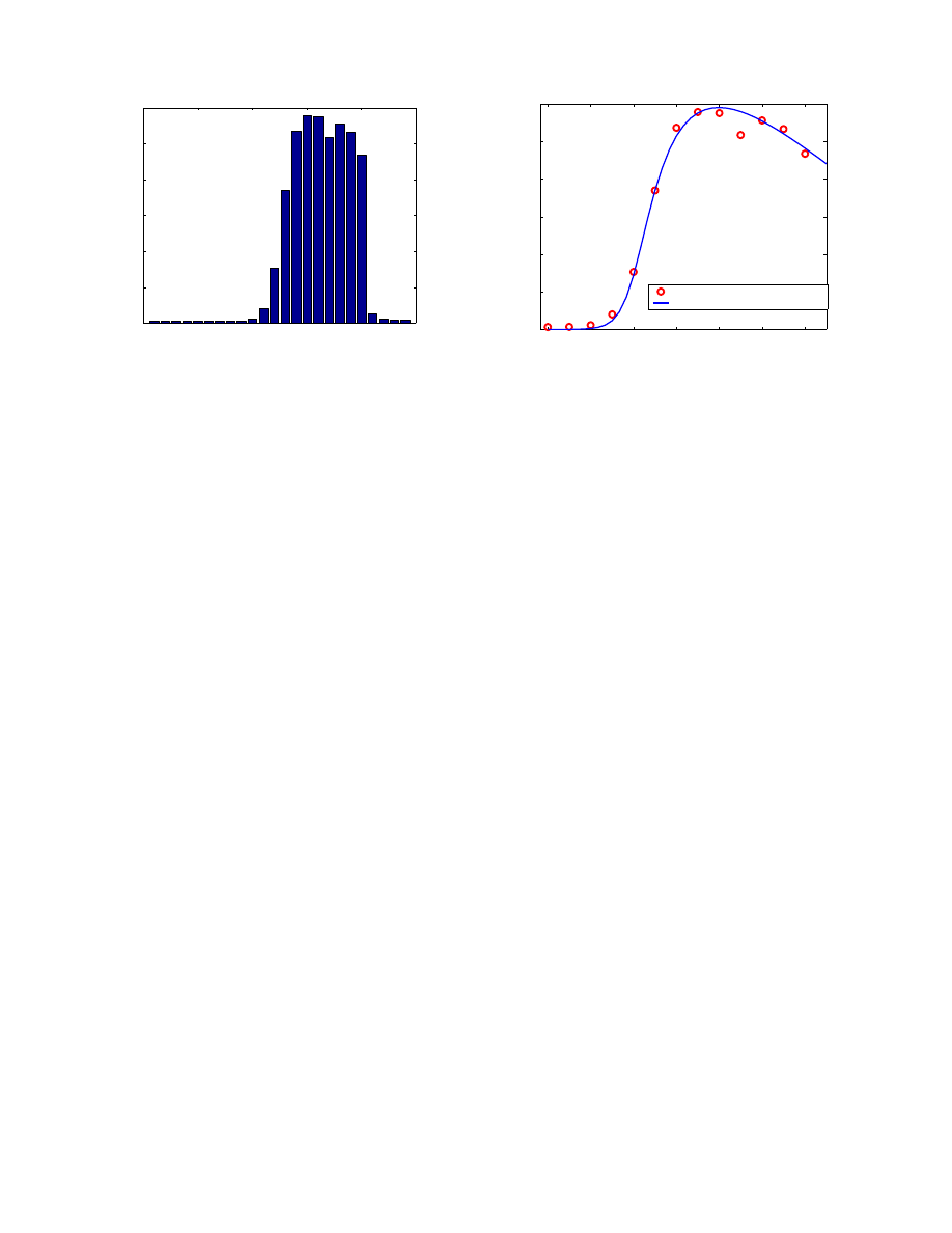
We vary the infection delay time D(t) to capture the

slowed down worm infection process. Let p(t) = J(t)/N
and X(t) be a random variable such that

X(t) ∼ N (k

1

p(t)

n

, k

2

p(t)

n

)

(11)

where N (µ, σ

2

) is the normal distribution with mean value

µ and variance σ

2

; k

1

, k

2

, n are model parameters.

In our simulation, we use the following equation to gener-

ate the infection delay time D(t) for each worm copy:

D(t) = D(0) + Y (t),

(12)

where D(0) is the base infection delay time and Y (t) is de-
rived by

Y (t) =

X(t) X(t) > 0
0

X(t) < 0

(13)

The normal distribution here is used to simulate the ran-

domness in the scan process of each worm copy. The power
exponent n in (11) is used to adjust the sensitivity of the
infection delay time D(t) to the number of infected hosts
J(t).

5.2

Simulation experiments

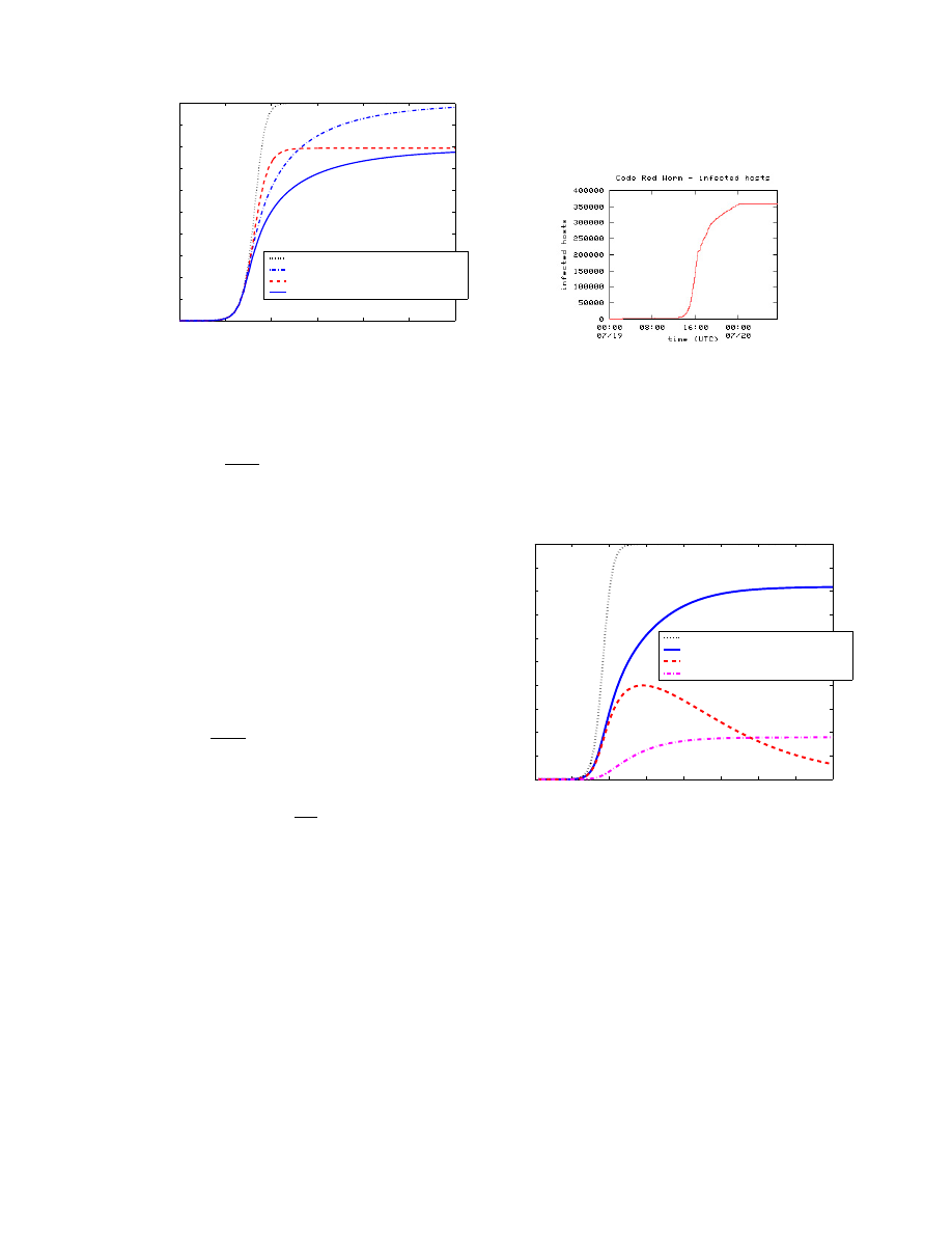
We simulate four scenarios. The first one is the classical

simple epidemic model (1), the same as used in [31] and [17,
32, 34]. It does not consider the two factors discussed in
this paper and can be simulated from our model by letting
D(t) = D(0) and a = 0. In the second scenario, we consider
only the decreased infection rate by using a = 0 and D(t)
as in (12). In the third scenario, we consider the effects

of patching and filtering but with constant infection rate
by using D(t) = D(0) and a = 0.5. In the last scenario we
use the two-factor worm model, allowing both immunization
and decreased infection rate, i.e., D(t) as in (12) and a =
0.5. For each scenario, we run the simulation 100 times and
derive the mean value of the number of infected hosts at
each time t, E[J(t)]. The E[J(t)] of these four scenarios are
plotted in Fig. 5 as functions of time t (The other simulation
parameters are: N = 1000000, D(0) = 10,k

1

= 150, k

2

=

70, n = 2; 10 initially infected hosts).

For the purpose of comparison, we plot the Fig. 2 again

right beside our simulation results Fig. 5. Comparing our
two-factor worm model simulation curve (the blue solid line
in Fig. 5) with the observed Code Red data in Fig. 6, we
observe that, by considering the removal processes and the
worm decreased infection rate, we can match the observed
data better than the original Code Red worm simulation
(the black dotted line in Fig. 5). In the beginning, the num-
ber of infected hosts, J(t), increases exponentially. However,
the propagation speed decreases when the total number of
infected hosts reaches only about 50% of the population.
The decreasing of propagation speed happens much earlier
than the original Code Red simulation. For future Internet
worms, by adjusting the parameters in our simulation, we
can adjust the curve to match real data and then understand
more of the characteristics of the worms we investigate.

We further investigate how variable each simulation is

among the 100 simulation runs of the two-factor model. By
using the maximum and minimum values for the number
of infected hosts at each time t, we derive two envelope
curves that contain all these 100 curves. These two envelope
curves are so close to each other that we can’t distinguish
them from a figure. The maximum difference between these
two curves is only 0.227% to the population size N . In
other words, the worm propagation is almost a determinis-
tic process — it’s the reason why we can use deterministic
differential equation (9) to model large-scale Internet worm
propagation, which is essentially a stochastic process.

The reason why random events have so little effect on

the worm propagation is that the population is huge (1 mil-
lion hosts) and each worm copy infects others independently.
From the whole worm propagation point of view, these huge
number of random events will eventually average out each
other.

6.

NUMERICAL ANALYSIS OF THE TWO-
FACTOR WORM MODEL

The two-factor worm model (9) is a general worm model

with several undetermined dynamic parameters β(t),R(t)
and Q(t). If we assume the infection rate β(t) to be con-
stant and do not consider the removal process from sus-
ceptible population, i.e., Q(t) = 0, we derive exactly the
Kermack-Mckendrick model (5) when R(t) = γI(t) [3]. For
the general two-factor worm model, we can’t get closed-form
analytical solutions. Instead, we analyze the model based on
the numerical solutions of the differential equation by using
Matlab Simulink [25] .

First we need to determine the dynamical equations de-

scribing R(t),Q(t) and β(t) in the two-factor worm model
(9). For the removal process from infectious hosts, we use
the same assumption as what Kermack-McKendrick model

0

100

200

300

400

500

600

0

1

2

3

4

5

6

7

8

9

10

x 10

5

Code Red propagation simulation

time: t

Total number of infected hosts J(t)

Original Code Red simulation
Consider slowing down of infection rate
Consider human countermeasures
Two−factor worm model

Figure 5: Code Red worm simulation based
on different models.

Figure 6:

Number of infected

hosts (from caida.org)

uses:

dR(t)

dt

= γI(t).

(14)

The removal process from susceptible hosts is more com-

plicated. At the beginning of the worm propagation, most
people don’t know there exists such a kind of worm. Conse-
quently the number of removed susceptible hosts is small and
increases slowly. As more and more computers are infected,
people gradually become aware of this worm and the im-
portance of defending against it. Hence the speed of immu-
nization increases fast as time goes on. The speed decreases
as the number of susceptible hosts shrinks and converges to
zero when there are no susceptible hosts available.

From the above description, the removal process of the

susceptible hosts looks similar to a typical epidemic propa-
gation. Thus we will use the classical simple epidemic model
(1) to model it:

dQ(t)

dt

= µS(t)J(t).

(15)

Last, we model the decreased infection rate β(t) by the

equation:

β(t) = β

0

[1

− I

(t)

N

]

η

,

(16)

where β

0

is the initial infection rate. The exponent η is

used to adjust the infection rate sensitivity to the number
of infectious hosts I(t). η = 0 means constant infection rate.

Using the assumptions above on Q(t), R(t) and β(t), we

write down the complete differential equations of the two-
factor worm model:


























dS(t)/dt = −β(t)S(t)I(t) − dQ(t)/dt

dR(t)/dt = γI(t)
dQ(t)/dt = µS(t)J(t)

β(t) = β

0

[1

− I(t)/N]

η

N = S(t) + I(t) + R(t) + Q(t)

I(0) = I

0

N; S(0) = N − I

0

; R(0) = Q(0) = 0;

(17)

For parameters N = 1, 000, 000, I

0

= 1, η = 3, γ = 0.05,

µ = 0.06/N , and β

0

= 0.8/N , we obtain the numerical

solutions of two-factor worm model (17) and plot them in
Fig. 7. The figure illustrates the behavior of J(t) = I(t) +

R(t), I(t), and Q(t) as functions of time t. For comparison,
we also plot the number of infected hosts J(t) of the classical
simple epidemic model (1) in this figure. The classical simple
epidemic model (1) can be derived from the two-factor worm
model (17) by simply setting η = 0, γ = 0, and µ = 0.

0

10

20

30

40

50

60

70

80

0

1

2

3

4

5

6

7

8

9

10

x 10

5

Two−factor worm model numerical solution

time: t

number of hosts

Classical simple epidemic model: J(t)
Infected hosts: J(t)=I(t)+R(t)
Infectious hosts: I(t)
Removed hosts from susceptible: Q(t)

Figure 7:

Numerical solution of two-factor worm

model

Comparing the two-factor model solution J(t) in Fig. 7

with the number of infected hosts in our Code Red worm
simulation Fig. 5, we can see that they are consistent and
well matched.

Figure 7 shows that the number of infectious hosts I(t)

reaches its maximum value at t = 29. From then on it
decreases because the number of removed infectious hosts in
a unit time is greater than the number of newly generated
infectious hosts at the same time.

We can explain this phenomenon by analyzing the two-

factor model equation (17). From (17) we can derive

dI(t)/dt = β(t)S(t)I(t) − dR(t)/dt

=

[β(t)S(t) − γ]I(t)

(18)

The number of susceptible hosts, S(t), is a monotonically

04:00

09:00

14:00

19:00

00:00

04:00

0

2

4

6

8

10

12

x 10

4

UTC hours (July 19 − 20)

number of unique sources

Code Red scan unique source IP data

two x.x.0.0/16 networks
Code Red scans per hour

Figure 8: Observed Code Red scan unique
sources hour-by-hour

12:00

14:00

16:00

18:00

20:00

22:00

00:00

0

2

4

6

8

10

12

x 10

4

UTC hours (July 19 − 20)

Number of infectious hosts

Comparison between model and observed data

Observed Code Red infectious hosts
two−factor worm model: I(t)

Figure 9:

Comparison between observed

data and our model

decreasing function of time. The maximum number of in-
fectious hosts, max I(t), will be reached at time t

c

when

S(t

c

) = γ/β(t

c

). β(t)S(t) − γ < 0 for t > t

c

, thus I(t)

decreases after t > t

c

.

The behavior of the number of infectious hosts I(t) in Fig.

7 can explain why the Code Red scan attempts dropped
down during the last several hours of July 19th [13, 16].
The data collected by Smith [16] and Eichman [13] contain
the number of the Code Red infectious sources that sent
out scans during each hour. It tells us how many computers
were still infectious during each hour on July 19th, thus the
number of observed infectious sources corresponds to I(t)
in our model. We plot the average values of these two data
sets in Fig. 8.

We plot in Fig. 9 both the observed data in Fig. 8 and

the I(t) derived from our model as shown in Fig. 7 (we
use the observed data from July 19th 12:00 to 00:00 UTC.
Code Red worm stopped propagation after 00:00 UTC July
20th). Figure 9 shows that they are matched quite well.
The classical simple epidemic model (1) can’t explain the
dropping down of Code Red propagation during the last
several hours of July 19th.

From the simple epidemic model (Fig. 4) and observed

data (Fig. 1), the authors in [31] concluded that Code Red
came to saturating around 19:00 UTC July 19th — almost
all susceptible IIS servers online on July 19th have been
infected around 19:00 UTC. However, the numerical solution
of our model, as shown in Fig. 7, shows that only roughly
60% of all susceptible IIS servers online have been infected
around that time.

7.

CONCLUSION

In this paper, we present a more accurate Internet worm

model and use it to model Code Red worm propagation.
Since Internet worms are similar to viruses in epidemic re-
search area, we can use epidemic models to model Inter-
net worms.

However, epidemic models are not accurate

enough. They can’t capture some specific properties of In-
ternet worms. By checking the Code Red worm incident
and networks properties, we find that there are two major
factors that affect an Internet worm propagation: one is the

effect of human countermeasures against worm spreading,
like cleaning, patching, filtering or even disconnecting com-
puters and networks; the other is the slowing down of worm
infection rate due to worm’s impact on Internet traffic and
infrastructure. By considering these two factors, we derive
a new general Internet worm model called two-factor worm
model. The simulations and the numerical solutions of the
two-factor worm model show that the model matches well
with the observed Code Red worm data of July 19th 2001.

In our two-factor worm model, the increasing speed of

the number of infected hosts will begin to slow down when
only about 50% of susceptible hosts have been infected. It
explains the earlier slowing down of the Code Red infection
in July 19th (Fig. 2). The number of current infected hosts
I(t) in Fig. 7 matches the corresponding observed data [13,
16] quite well as shown in Fig. 9. It explains why Code
Red scans dropped down during the last several hours of
July 19th, while previous worm models can’t explain such
phenomenon.

Due to the two factors that affect an Internet worm prop-

agation, the exponentially increased propagation speed is
only valid for the beginning phase of a worm. If we use
the traditional epidemic model to do a worm prediction, we
will always overestimate the spreading and damages of the
worm.

The two-factor worm model is a general Internet worm

model for modeling worms without topology constraint. It
isn’t just a specific model for Code Red. The slowing down
of worm infection rate will happen when the worm ram-
pantly sweeps the whole Internet and causes some troubles
to the Internet traffic and infrastructure, like what Code
Red worm and Nimda worm did [7, 10, 33]. Human coun-
termeasures, like cleaning, patching, filtering, or disconnect-
ing computers, play a major role in all kinds of viruses
or worms propagations no matter how fast or slow these
viruses or worms propagate. Human countermeasures will
successfully slow down and eventually eliminate viruses or
worms propagation. In real world, there are many viruses
and worms coming out almost every day, but few of them
show up and propagate seriously on Internet. Eventually all
of them pass away due to human countermeasures. Most
viruses and worms are not so contagious as Code Red and

Nimda. After the cleaning and patching rate exceeds the
viruses or worms propagation rate, those viruses and worms
will gradually disappear from the Internet circulation.

However, Internet worm models have their limitations.

For example, the two-factor worm model as well as other
worm models are only suitable for modeling a continuously
spreading worm, or the continuously spreading period of
a worm.

They can’t predict those arbitrary stopping or

restarting events of a worm, such as the stopping of Code
Red propagation on 00:00 UTC July 20th 2002 and its restart-
ing on August 1st — we can only find such events through
manually code analysis.

In our two-factor worm model (17), we select parame-

ters, γ, µ, β

0

, n and η, such that the numerical solutions

can match with the observed Code Red data. Even for the
simple epidemic model (1), we still need to determine the
parameter β before using it. For the prediction and dam-
age assessment of future viruses and worms, we need to do
more research to find an analytical way to determine these
parameters beforehand.

8.

REFERENCES

[1] R. M. Anderson, R.M. May. Infectious diseases of

humans: dynamics and control. Oxford University
Press, Oxford, 1991.

[2] H. Andersson, T. Britton. Stochastic Epidemic Models

and Their Statistical Analysis. Springer-Verlag, New
York, 2000.

[3] N. T. Bailey. The Mathematical Theory of Infectious

Diseases and its Applications. Hafner Press, New
York, 1975.

[4] CERT Advisory CA-2001-23. Continued Threat of the

“Code Red” Worm.
http://www.cert.org/advisories/CA-2001-23.html

[5] CERT Advisory CA-2000-04. Love Letter Worm.

http://www.cert.org/advisories/CA-2000-04.html

[6] CERT Advisory CA-1999-04. Melissa Macro Virus.

http://www.cert.org/advisories/CA-1999-04.html

[7] Cisco Security Advisory: “Code Red” Worm -

Customer Impact.
http://www.cisco.com/warp/public/707/cisco-code-
red-worm-pub.shtml

[8] Cisco Tech. notes: Dealing with mallocfail and High

CPU Utilization Resulting From the “Code Red”
Worm.

http://www.cisco.com/warp/public/63/

ts codred worm.shtml

[9] CNN news. “Code Red” worm “minimized” – for now.

http://www.cnn.com/2001/TECH/internet
/08/02/code.red.worm/

[10] J. Cowie, A. Ogielski, B. Premore and Y. Yuan.

Global Routing Instabilities during Code Red II and
Nimda Worm Propagation.
http://www.renesys.com/projects/bgp instability/

[11] eEye Digital Security. .ida “Code Red” Worm.

http://www.eeye.com/html/Research/Advisories/
AL20010717.html

[12] eEye Digital Security. CodeRedII Worm Analysis.

http://www.eeye.com/html/Research/Advisories/
AL20010804.html

[13] K. Eichman. Mailist: Re: Possible CodeRed

Connection Attempts.
http://lists.jammed.com/incidents/2001/07/0159.html

[14] eWeek news. Code Red Lessons, Big and Small.

http://www.eweek.com/article2/0,3959,113815,00.asp

[15] J. C. Frauenthal. Mathematical Modeling in

Epidemiology. Springer-Verlag, New York, 1980.

[16] D. Goldsmith. Maillist: Possible CodeRed Connection

Attempts.
http://lists.jammed.com/incidents/2001/07/0149.html

[17] T. Heberlein. Visual simulation of Code Red worm

propagation patterns.
http://www.incidents.org/archives/intrusions/
msg00659.html

[18] Incidents.org diary archive.

http://www.incidents.org/diary/july2001.php

[19] Netcraft Web Server Survey — June 2001.

http://www.netcraft.com/Survey/index-200106.html

[20] J. O. Kephart and S. R. White. Directed-graph

Epidemiological Models of Computer Viruses.
Proceedings of the IEEE Symposimum on Security and
Privacy, 343-359, 1991.

[21] J. O. Kephart, D. M. Chess and S. R. White.

Computers and Epidemiology. IEEE Spectrum, 1993.

[22] J. O. Kephart and S. R. White. Measuring and

Modeling Computer Virus Prevalence. Proceedings of
the IEEE Symposimum on Security and Privacy, 1993.

[23] R. Lemos. Virulent worm calls into doubt our ability

to protect the Net.
http://news.com.com/2009-1001-270471.html

[24] R. Lemos. Microsoft reveals Web server hole.

http://news.com.com/2100-1001-268608.html

[25] Matlab Simulink. The Mathworks, Inc.
[26] V. Misra, W. Gong and D. Towsley. A fluid based

analysis of a network of AQM routers supporting TCP
flows with an application to RED. Proceedings of
ACM/SIGCOMM, 151-160, 2000.

[27] D. Moore. The Spread of the Code-Red Worm.

http://www.caida.org/analysis/security/code-
red/coderedv2 analysis.xml

[28] C. Nachenberg. The Evolving Virus Threat. 23rd

NISSC Proceedings, Baltimore, Maryland, 2000.

[29] SilentBlade. Info and Analysis of the ’Code Red’.

http://www.securitywriters.org/library/texts/
malware/commu/codered.php

[30] E.H. Spafford. The internet worm incident. In

ESEC’89 2nd European Software Engineering
Conference, Coventry, United Kingdom, 1989.

[31] S. Staniford, V. Paxson and N. Weaver. How to Own

the Internet in Your Spare Time. 11th Usenix Security
Symposium, San Francisco, August, 2002.

[32] C. Wang, J. C. Knight and M. C. Elder. On Viral

Propagation and the Effect of Immunization.
Proceedings of 16th ACM Annual Computer
Applications Conference, New Orleans, LA, 2000.

[33] L. Wang, X. Zhao, D. Pei, R. Bush, D. Massey, A.

Mankin, S. Wu and L. Zhang. Observation and
Analysis of BGP Behavior under Stress. Internet
Measurement Workshop, France, November, 2002.

[34] N. Weaver. Warhol Worms: The Potential for Very

Fast Internet Plagues.
http://www.cs.berkeley.edu/˜nweaver/warhol.html