Statyka Wykład 2 St.7

Zbieżne układy sił

Płaski lub przestrzenny układ sił zbieżnych P₁, P₂, .. P_i, ..P_n przyłożonych do jednego punktu 0 można zastąpić jedną siłą wypadkową P przyłożoną w tymże punkcie i równą sumie geometrycznej tych sił (rys.14).

P₂ P = P₁₂ + P₃

P

P₁₂ = P₁ + P₂

P₃

P₁ 0 Rys.14

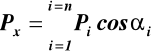
Analityczny sposób wyznaczania wypadkowej przestrzennego układu sił zbieżnych (rys.15).

z

P_i

P_i+1

γ_i

β_i

0 y

α_i

P_n P₂

P₁

x Rys.15

Składowe siły P_i na osie prostokątnego układu 0xyz (rys.16)

z

P_iz P_i P_iy y

P_ix

x Rys.16

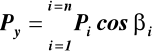
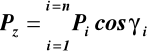
P_ix = P_icosα_i P_iy = P_icosβ_i P_iz = P_icosγ_i (13) St.8

(14)

Wartość liczbowa wypadkowej P określamy z (15) (rys.17)

z

P_z

γ P

α β

0 P_y y

P_x

x Rys.17

(15)

cosinusy kierunkowe określamy z (16)

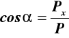
(16)

Przykład 2

Na punkt 0 działają trzy siły P₁, P₂, P₃.

Dane: P₁ = 15N, P₂ = 13N, P₃ = 17N

α₁ = 62⁰, β₁ = 70⁰, γ₁ = 35,5⁰; α₂ = 42⁰, β₂ = 81⁰, γ₂ =49,4 ⁰;

α₃ = 49⁰, β₃ = 68⁰, γ₃ = 49,1⁰;

Szukane: wartość liczbowa wypadkowej, wartości kątów α,β,γ.

Rozwiązanie

z (14)

z (15)

z (16)
α = 51,1⁰ St.9

cosβ = 0,305 β =72,2⁰, cosγ = 0,716 γ =44,2⁰

sprawdzenie czy obliczone kąty spełniają zależność (17)

cos²α + cos²β + cos²γ =1 (17)

cos²51,1⁰ + cos²72,2⁰ +cos²44,2⁰ = 1

1.0018 ≅ 1

Równowaga płaskiego i przestrzennego układu sił zbieżnych

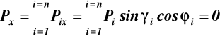
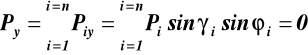
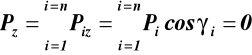
Warunki równowagi (równania równowagi)

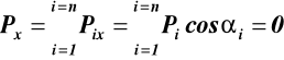
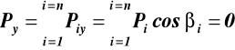
(18)

lub (rys.18) z

P_iz

γ_i P_i

α_i β_i

0 P_iy y

P_ix ϕ_i

P_ixy Rys.18

x

(19)

Przykład 3 St.10

Nieważkie pręty 0B, 0C i 0D połączone są przegubowo w punktach 0, B, C i D (rys.19)

Wyznaczyć: siły w prętach.

Dane: w punkcie 0 działa siła P₁ = 18N, której rzut na płaszczyznę 0xy tworzy z osią x kąt *₁ = 41⁰,

natomiast γ₁ = 129⁰, γ_s = 35⁰, β_s = 49⁰ (rys.19).

z

D

γ_s

B

β_s γ₁

C 0 y

*₁ P_1xy P_1y

P_1x

x P_1z P₁

Rys.19

Na rysunku 20 przedstawiono oddziaływanie prętów 0C, 0D i 0B

na węzeł 0, S_0D

90⁰-γ_s z S_0B

S_0C 0 y

x P Rys.20

zaznaczono również działanie siły P

Równania równowagi węzła 0 St.11

z (19)

z (19) i (rys.21)

(a)

z (19)

(b)

z (19)

S_0D = 13,83N (c)

Wstawiając (c) do (a) i (b) otrzymujemy

10,56 - S_0B - 13,83*0,433 = 0 S_0B = 4,57N

9,18 - S_0C - 0,376*13,83 = 0 S_0C = 3,98N

S_0Dxy

S_0Dx

(270⁰ - β_s)

S_0Dy 0 y

x Rys.21

S_0Dxy = S_0D*sinγ_s S_0Dx = S_0Dxy*cos(270⁰ - β_s)

---