26

3 Multidimensional NMR Spectroscopy

© Gerd Gemmecker, 1999

Models used for the description of NMR experiments

1. energy level diagram: only for polarisations, not for time-dependent phenomena

2. classical treatment (B

LOCH EQUATIONS

): only for isolated spins (no J coupling!)

3. vektor diagram: pictorial representation of the classical approach (same limitations)

4. quantum mechanical treatment (density matrix): rather complicated; however, using

appropriate simplifications and definitions – the product operators – a fairly easy and correct

description of most experiments is possible

3.1. B

LOCH

Equations

The behaviour of isolated spins can be described by classical differential equations:

dM/dt =

γ

M(t) x B(t) - R{M(t) -M0}

[3-1]

with M

0

being the B

OLTZMANN

equilibrium magnetization and R the relaxation matrix:

x y z

R =













1/Τ2

0

0

0

1/Τ2

0

0

0

1/Τ1

The external magnetic field consists of the static field B

0

and the oscillating r.f. field B

rf

:

B(t) = B

0

+ B

rf

[3-2]

B

rf

= B

1

cos(

ω

t +

φ

)e

x

[3-3]

The time-dependent behaviour of the magnetization vector corresponds to rotations in space (plus

relaxation), with the B

x

and B

y

components derived from r.f. pulses and B

z

from the static field:

dMz/dt =

γ

BxMy -

γ

ByMx -(Mz-M

0

)/T

1

[3-4]

dMx/dt =

γ

ByMz -

γ

BzMy - Mx/T

2

[3-5]

dMy/dt =

γ

BzMx -

γ

BxMz - My/T

2

[3-6]

Product operators

To include coupling a special quantum mechanical treatment has to be chosen for description. An

operator, called the spin density matrix

ρ

(t), completely describes the state of a large ensemble of

27

spins. All observable (and non-observable) physical values can be extracted by multiplying the

density matrix with their appropriate operator and then calculating the trace of the resulting matrix.

The time-dependent evolution of the system is calculated by unitary transformations (corresponding

to "rotations") of the density matrix operator with the proper Hamiltonian H (including r.f. pulses,

chemical shift evolution, J coupling etc.):

ρ

(t') = exp{iHt}

ρ

(t) exp{-iHt}

(for calculations these exponential operators have to be expanded into a Taylor series).

The density operator can be written als linear combination of a set of basis operators. Two specific

bases turn out to be useful for NMR experiments:

- the real Cartesian product operators I

x

, I

y

and I

z

(useful for description of observable

magnetization and effects of r.f. pulses, J coupling and chemical shift) and

- the complex single-element basis set I

+

, I

-

, I

α

and I

β

(raising / lowering operators, useful for

coherence order selection / phase cycling / gradient selection).

Cartesian Product operators

Lit. O.W. Sørensen et al. (1983), Prog. NMR. Spectr. 16, 163-192

Single spin operators

correspond to magnetization of single spins, analogous to the classical macroscopic magnetization

M

x

, M

y

, M

z.

I

x

, I

y

(in-phase coherence, observable)

I

z

(z polarisation, not observable)

Two-spin operators

2I

1x

I

2z

, 2I

1y

I

2z

, 2I

1z

I

2x

, 2I

1z

I

2y

(antiphase coherence, not observable)

2I

1z

I

2z

(longitudinal two-spin order, not observable)

2I

1x

I

2x

, 2I

1y

I

2x

, 2I

1x

I

2y

, 2I

1y

I

2y

(multiquantum coherence, not observable)

28

Sums and differences of product operators

2 I

1x

I

2x

+ 2 I

1y

I

2y

= I

1

+

I

2

-

+ I

1

-

I

2

+

zero-quantum coherence

2 I

1y

I

2x

- 2 I

1x

I

2y

= I

1

+

I

2

-

- I

1

-

I

2

+

(not observable)

2 I

1x

I

2x

- 2 I

1y

I

2y

= I

1

+

I

2

+

+ I

1

-

I

2

-

double-quantum coherence

2 I

1x

I

2y

+ 2 I

1y

I

2x

= I

1

+

I

2

+

- I

1

-

I

2

-

(not observable)

The single-element operators I

+

and I

-

correspond to a transition from the m

z

= -

1

/

2

to the m

z

= +

1

/

2

state and back, resp., hence "raising" and "lowering operator". Products of three and more operators

are also possible.

Only the operators I

x

and I

y

represent observable magnetization. However, other terms like antiphase

magnetization 2 I

1x

I

2z

can evolve into observable terms during the acquisition period.

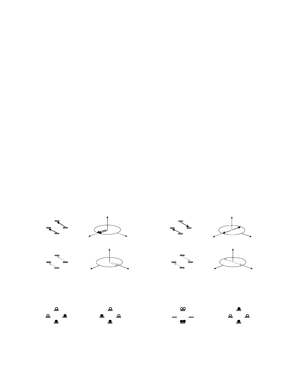
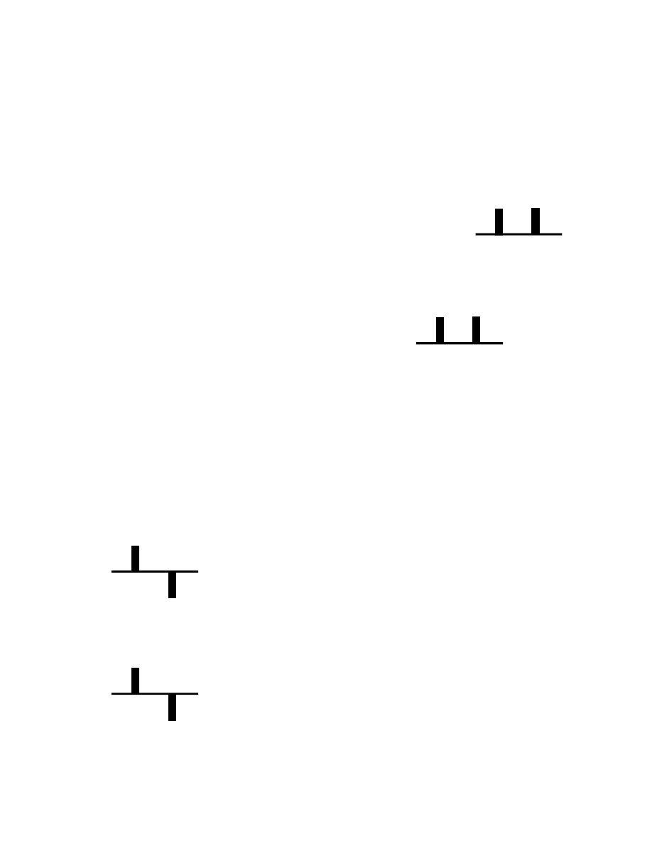
Pictorial representations of product operators

(cf. the paper in Progr. NMR Spectrosc. by Sørensen et al.)

αα

αα

αα

αα

αα

αα

αα

αα

αβ

αβ

αβ

αβ

αβ

αβ

αβ

αβ

βα

βα

βα

βα

βα

βα

βα

βα

ββ

ββ

ββ

ββ

ββ

ββ

ββ

ββ

I

x

I

1 z

I

2 z

2I I

1 z

2 z

I +I

1 z

2 z

I

y

I I

1 x

2 z

I I

1 y

2 z

x

x

x

x

y

y

y

y

z

z

z

z

coherences

polarisations

29

In the energy level diagrams for coherences, the single quantum coherences I

x

and I

y

are

symbolically depicted as black and gray arrows. Both arrows in each two-spin scheme (for the

coupling partner being

α

or

β

) belong to the same operator; in the vector diagrams these two species

either align (for in-phase coherence) or a 180° out of phase (antiphase coherence). In the NMR

spectrum, these two arrows / transitions correspond to the two lines of the dublet caused by the J

coupling between the two spins. The term 2I

1x

I

2z

is called antiphase coherence of spin 1 with

respect to spin 2.

For the populations, filled circles represent a population surplus, empty circles a population deficit

(with respect to an even distribution). I

1z

and I

2z

are polarisations of one sort of spins only, I

1z

+I

2z

is

the normal B

OLTZMANN

equilibrium state, and 2 I

1z

I

2z

is called longitudinal two-spin order (with the

two spins in each molecule preferentially in the same spin state).

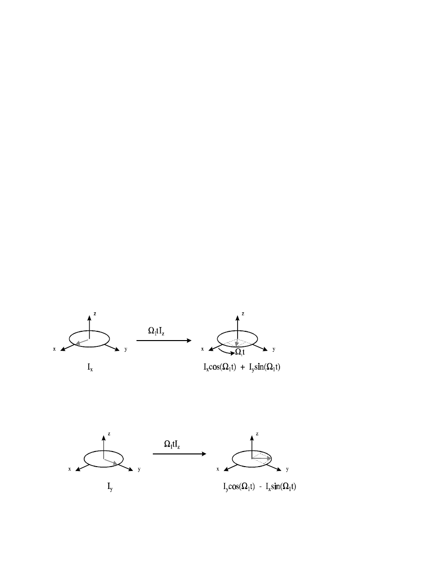
Evolution of product operators

Chemical shift

Ω

1

tI

z

I

1x

→

I

1x

cos(

Ω

1

t) + I

1y

sin(

Ω

1

t)

[3-7]

Ω

1

tI

1z

I

1y

→

I

1y

cos(

Ω

1

t) - I

1x

sin(

Ω

1

t)

[3-8]

30

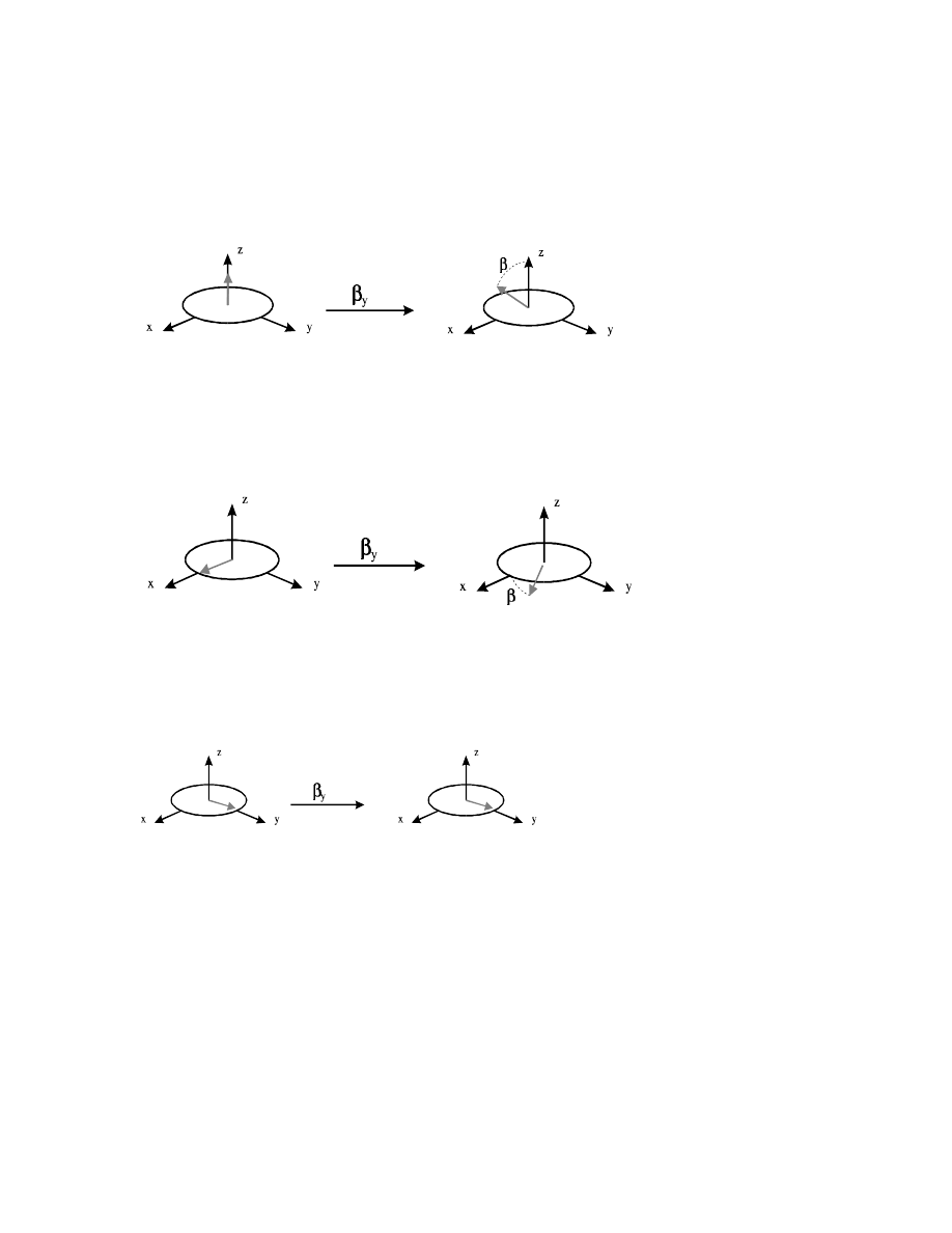
Effect of r.f. pulses

β

I

y

I

1z

→

I

1z

cos

β

+ I

1x

sin

β

[3-9]

β

I

y

I

1x

→

I

1x

cos

β

- I

1z

sin

β

[3-10]

β

I

y

I

1y

→

I

1y

The effects of x and z pulses can be determined by cyclic permutation of x, y, and z. All rotations

obey the "right-hand rule", i.e., with the thumb of the right (!) hand pointing in the direction of the

r.f. pulse, the curvature of the four other fingers indicate the direction of the rotation.

31

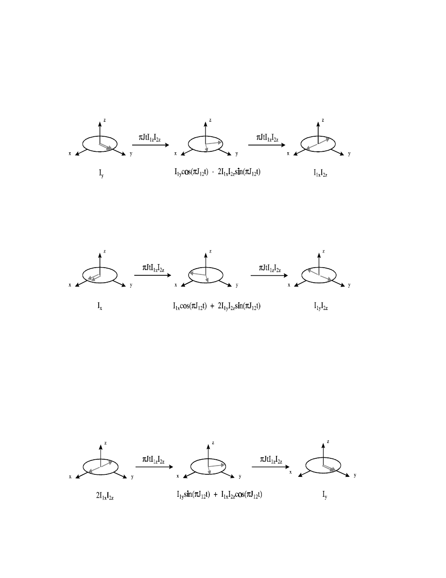
Scalar coupling

π

JtI

1z

I

2z

I

1x

→

I

1x

cos(

π

Jt) + 2I

1y

I

2z

sin(

π

Jt)

[3-11]

π

JtI

1z

I

2z

I

1y

→

I

1y

cos(

π

Jt) - 2I

1x

I

2z

sin(

π

Jt)

[3-12]

π

JtI

1z

I

2z

I

1z

→

I

1z

(i.e., I

1z

does not evolve J coupling!)

π

JtI

1z

I

2z

2I

1x

I

2z

→

I

1y

sin(

π

Jt) + 2I

1x

I

2z

cos(

π

Jt)

[3-13]

32

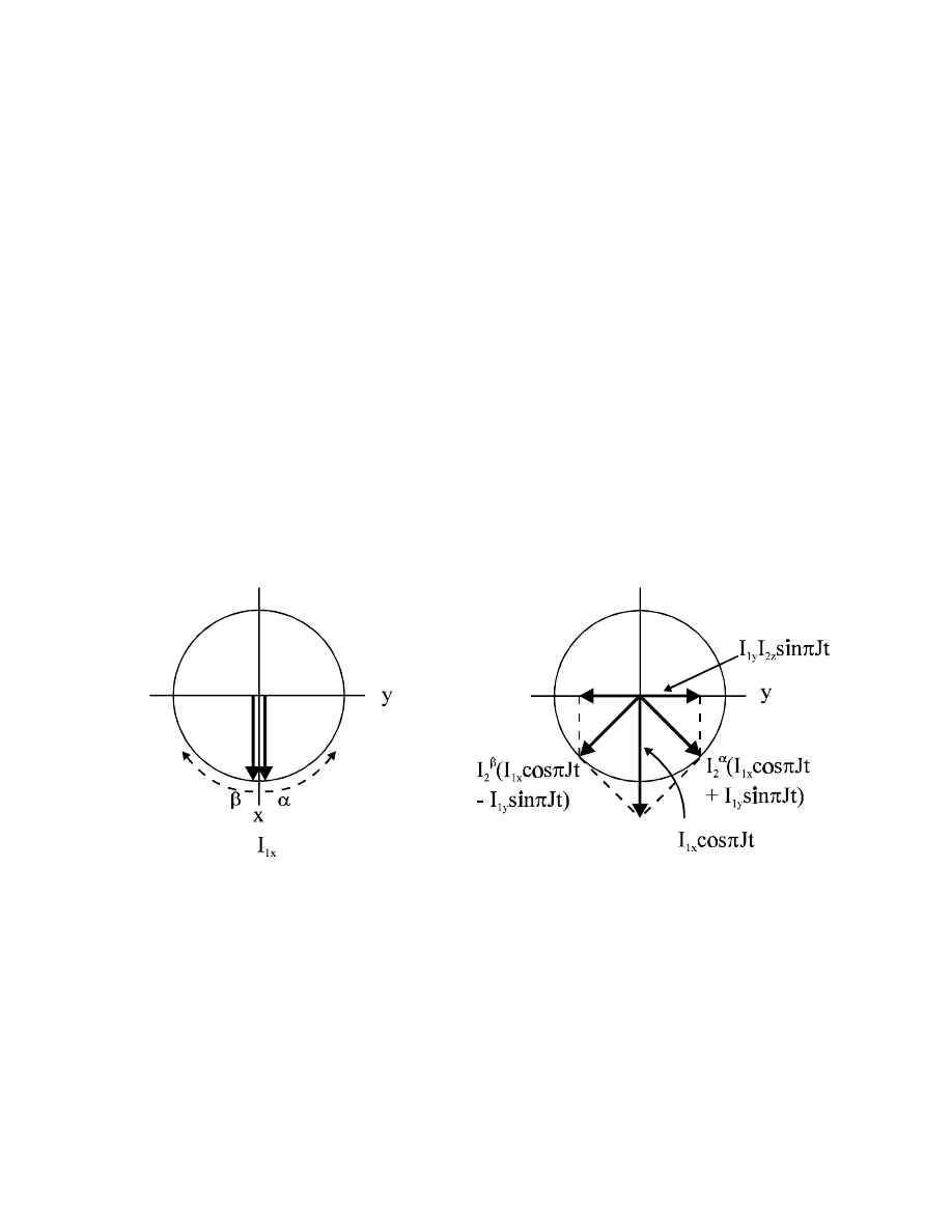
The antiphase term 2I

1y

I

2z

can be re-written using the single-element operators I

α

und I

β

:

2I

1y

I

2z

= I

1y

I

2

α

- I

1y

I

2

β

[3-14]

(2I

z

= I

α

- I

β,

I

α +

I

β = 11

;

I

α

und I

β

are called polarization operators

)

The antiphase state 2I

1y

I

2z

consists of two separate populations: for one half of the molecules in the

ensemble spin 1 is in +y coherence (when spin 2 is in the

α

state), for the other half spin 1 is in -y

coherence (with spin 2 in the

β

state); "spin 1 is in antiphase with respect to spin 2".

Such an antiphase state can develop from I

1x

when spin 1 is J-coupled to spin 2. This leads to a

dublet for spin 1, i.e., it splits into two lines with an up- and downfield shift by

J

/

2

, depending on the

spin state of the coipling partner, spin 2. If we wait long enough (

1

/

2

J

), then the frequency

difference of J between the dublet lines (I

1x

I

2

α

and I

1x

I

2

β

) has brought them 180° out of phase

("antiphase"), as shown in the vector diagram.

This is an oscillation between I

1x

in-phase coherence and 2I

1y

I

2z

antiphase coherence. The antiphase

component evolves with sin(

πJt) and then refocusses back to -I

1x

in-phase coherence (after t=

1

/

J

).

Single-element operators

In some cases (phase cycling, gradient coherence selection) it is necessary to use operators with a

defined coherence order (Eigenstates of coherence order). Coherence order describes the changes in

quantum numbers m

z

caused by the coherence. A spin-

1

/

2

system (no coupling) can assume two

coherent states: a transition from

α

(m

z

=+

1

/

2

) to

β

(m

z

=-

1

/

2

), i.e., a change (coherence order) of -1.

33

This can be described by the lowering operator I

-

= |

β

><

α

|, the coherent transition from the

β

to

α

state by the raising operator I

+

= |

α

><

β

| (coherence order +1).

The real Cartesian operators I

x

and I

y

correspond

to mixtures of both coherence orders,

±

1, although

they are more useful for directly corresponding to the observable x and y components of the

magnetization. Their relationship with the complex I

±

operators is simple:

I

+

= I

x

+ iI

y

raising operator

I

x

=

1

/

2

(I

+

+ I

-

)

I

-

= I

x

- iI

y

lowering operator

I

y

= -

i

/

2

(I

+

- I

-

)

I

α

=

1

/

2

1 + I

z

polarisation operator (

α

)

I

z

=

1

/

2

(I

α

- I

β

)

I

β

=

1

/

2

1 - I

z

polarisation operator (

β

)

1 = I

α

+ I

β

The effect of r.f. pulses (here: an x pulse with flip angle

ϕ

) on single-element operators is as follows:

ϕ

x

I

+/-

→

I

+/-

cos

2

{

ϕ

/2} + I

-/+

sin

2

{

ϕ

/2} (+/- iI

z

sin{

ϕ

})

[3-15]

ϕ

x

I

β

→

I

β

cos

2

{

ϕ

/2} + I

α

sin

2

{

ϕ

/2} + (1/2)sin{

ϕ

}[I

+

- iI

-

]

[3-16]

ϕ

x

I

α

→

I

α

cos

2

{

ϕ

/2} + I

β

sin

2

{

ϕ

/2} - (1/2)sin{

ϕ

}[I

+

- iI

-

]

[3-17]

Generally it is easier to calculate the effects of r.f. pulses on Cartesian operators and then use the

conversion rules to get the single-element version.

34

Signal phase, In-phase and antiphase signals

For a single spin I

1

one gets the following signal during acquisition with receiver reference phase x:

I

x

→

I

x

cos (

Ω

Ω

t ) + I

y

sin (

Ω

t)

I

y

→

I

y

cos (

Ω

t ) - I

x

sin (

Ω

Ω

t)

These two signals are 90° out of phase (also after FT), which is indicated by one I

x

component

having a sine, the other one a cosine modulation.

For a spin I

1

coupled to another spin I

2

one gets the following signal during acquisition (neglecting

chemical shift evolution):

I

x

→

I

x

cos (

Ω

t) + I

y

sin (

Ω

t)

→

I

x

cos (

Ω

Ω

t) cos (

ππ

Jt) + 2 I

1y

I

2z

cos (

Ω

t) sin(

π

Jt)

+ I

y

sin (

Ω

t) cos (

π

Jt) - 2 I

1x

I

2z

sin (

Ω

t)

sin(

π

Jt)

the detected x component corresponds to an in-phase dublet with splitting J, i.e., lines with intensity

1

/

2

at positions (

Ω

+

J

/

2

) and (

Ω

-

J

/

2

)

(

π

Jt =

2

π

J

/

2

t ).

cos

α

cos

β

=

1

/

2

[cos (

α+β

) + cos (

α−β

)]

2 I

1x

I

2z

→

2 I

1x

I

2z

cos (

Ω

t) + 2 I

1y

I

2z

sin (

Ω

t)

→

2 I

1x

I

2z

cos (

Ω

t) cos(

π

Jt) + I

y

cos (

Ω

t) sin (

π

Jt)

+ 2 I

1y

I

2z

sin (

Ω

t) sin(

π

Jt) - I

x

sin (

Ω

Ω

t) sin (

ππ

Jt)

this tiem the x component corresponds to an anti-phase dublet with splitting J, i.e., lines with

intensities of

1

/

2

and -

1

/

2

at positions (

Ω

+

J

/

2

) and (

Ω

-

J

/

2

)

:

35

sin

α

sin

β

=

1

/

2

[cos (

α+β

) - cos (

α−β

)]

In the same way, I

y

leads to an in-phase dublet 90° out of phase (=dispersive) and 2 I

1y

I

2z

to a

dispersive anti-phase dublet.

Some applications

1. For solvent signal suppression in 1D spectra, the Jump-Return sequence can be used:

90°(x) -

τ

- 90°(x) - acquisition

Calculate the excitation profile with product operator formalism!

2. What happens to chemical shift evolution during this sequence, and what about J coupling?

Calculate!

90°(x) -

τ

- 180°(x) -

τ

-

90°(x) -

τ

- 180°(y) -

τ

-

36

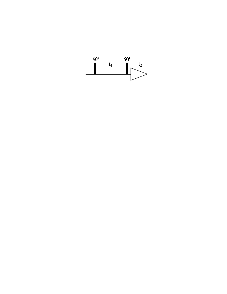
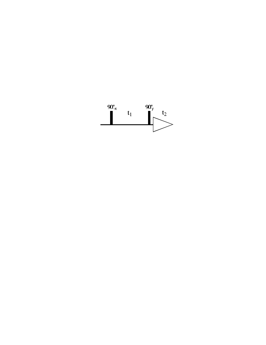
A simple 2D experiment (COSY)

Let's calculate the result of this two-pulse COSY sequence for a single spin I:

y

y

The first 90°y pulse creates transverse magnetization, which then evolves under the influence of

chemical shift and J coupling during the delay t

1

, after the second 90°

y

pulse we get:

90°

y

Ω

t

1

90°

y

I

z

→

I

x

→

I

x

cos(

Ω

t

1

)

→ −

I

z

cos(

Ω

t

1

)

+ I

y

sin(

Ω

t

1

)

+ I

y

sin(

Ω

Ω

t

1

)

During the acquisition time t

2

the first component is not detectable (polarization I

z

), the other (bold)

term is a coherence which will evolve during t

2

as follows:

Ω

t

2

I

y

sin(

Ω

t

1

)

→

I

y

sin(

Ω

t

1

) cos(

Ω

t

2

)

- I

x

sin(

Ω

t

1

) sin(

Ω

t

2

)

If we compare this to a normal 1D spectrum (let's call the acquisition time again t

2

)

90°

y

Ω

t

1

I

z

→

I

x

→

I

x

cos(

Ω

t

2

)

+ I

y

sin(

Ω

t

2

)

we see that both signals correspond the real and imaginary part of a precession with frequency

Ω

during the acquisition time t

2

. The only difference between the 1D and the COSY spectrum – besides

a 90° phase shift (for the 1D, the absorptive and dispersive components are I

x

and I

y

, for the COSY

they are I

y

and -I

x

, resp.) – is the factor sin(

Ωt

1

) in the COSY terms. So far, this is just a constant

with a value somewhere between -1 and +1, depending on the chosen t

1

value (and on

Ω

, of course).

However, the result of the COSY sequence contains very similar factors for t

1

and t

2

, i.e., a sine or

cosine modulation with the argument

Ω

t

i

. Instead of a t

2

FT, we could also perform a FT in t

1

.

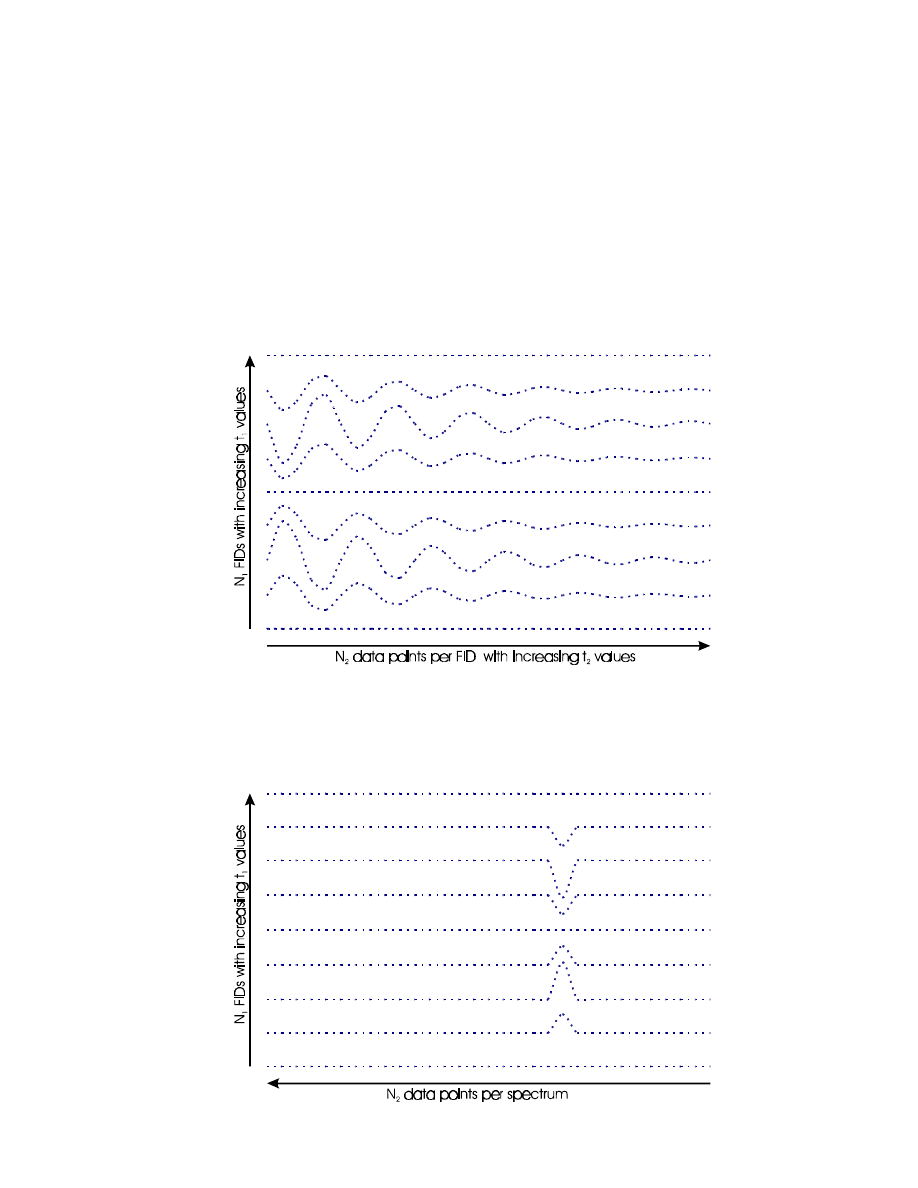
37

Of course, we have only data for a single t

1

value (the one we chose in the COSY sequence), but for

a FT we need to know a whole series of values of the oscillatory function, as we do for t

2

(all the

TD2 time domain data points sampled during the acquisition time, for t

2

=0, t

2

=DW, t

2

=2DW, …

t

2

=AQ

2

).

We can re-run the COSY sequence with a different setting for t

1

, and another one, etc., starting from

t

1

=0, then t

1

=DW, t

1

=2DW, … t

1

=AQ

1

(TD1 different t

1

values). Our complete data set now consists

of TD1 FIDs (with TD2 data points each):

We can now perform a "normal" FT along t

2

, converting the series of FIDs into a series of spectra,

which are all identical (with a signal at

Ω

), except for a modulation with sin(

Ωt

1

) along the t

1

dimension:

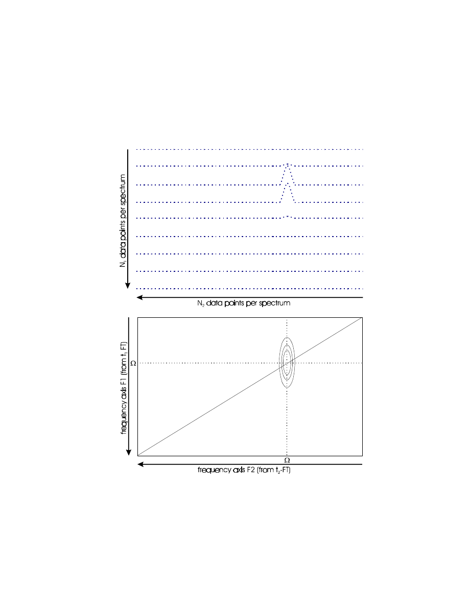
38

If we now read out single columns from our 2D data matrix, then we will generally get a pseudo-FID

A sin(

Ωt

1

) for each column, with A=0 where there is no signal in the F2 dimension (the frequency

dimension generated by the t

2

-FT) and with A

≠

0 where we have our signal (at

Ω

in F2).

From these pseudo-FIDs we can again generate a frequency spectrum by FT (now along the t

1

dimension), and will get a signal at the frequency

Ω

in this F1 dimension – in the column at

Ω

in F2:

This is a 2D COSY spectrum! – although not very interesting, since it contains just one diagonal

peak (=with identical chemical shift

Ω

in both dimensions), no more information than a simple 1D

spectrum.

39

In order to achieve a distinction between positive and negative

Ω

values (

Ω

=0 is in the center of

each dimension), a complex FT also in the indirect F1 dimension is required, i.e., the sine and the

cosine component. From our pulse sequence we get only

I

y

sin(

Ω

t

1

) cos(

Ω

t

2

) - I

x

sin(

Ω

t

1

) sin(

Ω

t

2

)

These are the two (real and imaginary) components for a t

2

value, but only the sine component in t

1

.

We have to re-run our complete set of TD1 t

1

increments with a slightly modified pulse sequence,

with the first pulse phase shifted by 90°:

90°

-x

Ω

t

1

90°

y

Ω

t

2

I

z

→

I

y

→

I

y

cos(

Ω

t

1

)

→

I

y

cos(

Ω

t

1

)

→

I

y

cos(

Ω

Ω

t

1

) cos(

Ω

Ω

t

2

) - I

x

cos(

Ω

Ω

t

1

) sin(

Ω

Ω

t

2

)

-I

x

sin(

Ω

t

1

)

+ I

z

sin(

Ω

t

1

)

+ I

z

sin(

Ω

t

1

)

We now get exactly the same terms as for the first COSY pulse sequence, only with a cosine

modulation. Combining the two data sets, we get four data points for each t

1

/t

2

combination:

I

y

sin(

Ω

t

1

) cos(

Ω

t

2

)

- I

x

sin(

Ω

t

1

) sin(

Ω

t

2

)

I

y

cos(

Ω

t

1

) cos(

Ω

t

2

) - I

x

cos(

Ω

t

1

) sin(

Ω

t

2

)

This is called a hypercomplex data point, and a 2D matrix of such data points contains all sine/cosine

combinations needed for a hypercomplex 2D-FT, yielding the frequency

Ω

including the correct sign

in both dimensions. There are different ways to acquire the equivalent of a hypercomplex data set:

- the S

TATES

(-R

UBEN

-H

ABERKORN

) method outlined here (first pulse phase x/y for each t

1

point)

- the TPPI (Time Proportional Phase Incrementation), which is analogous to the R

EDFIELD

trick

for single-channel acquisition (only real data points in t

1

, but twice as many, with half the time

increment

40

- echo-antiecho quadrature detection, which does not sample the real and imaginary (I

x

and I

y

)

components separately, but rather I

+

and I

-

(by coherence selction through phase cycling or

gradients) – which can then be easily converted into I

x

and I

y

by the computer

Magnitude mode spectra

Alternatively, one can only select either I

+

or I

-

during t

1

(i.e., only one data point per t

1

value), again

by phase cycling or gradients. This corresponds to either the spectrum or its mirror image in the

indirect dimension, so no quad images will occur. However, according to I

+

= I

x

+ iI

y

/ I

-

= I

x

- iI

y

these are complex components with no pure phase. The resulting spectrum cannot be phased to pure

absorptive lineschapes in F1 and hence has to be displayed in absolute value/magnitude or power

mode.

This was quite popular many years ago, when data storage and processing capacity were limited.

However, the S/N is only

1

/

2

(ca. 71 %) of a S

TATES

or TPPI spectrum of equal measuring time

and digital resolution, because the r.f. pulses create I

x

=

1

/

2

(I

+

+ I

-

) or I

y

= -

i

/

2

(I

+

- I

-

) at the

beginning of t

1

, so only 50 % of the signal is selected by the phase cycle or gradients. Worse even,

the very unfavourable magnitude or power mode lineshapes greatly reduce the spectral resolution,

even with optimized apodization functions.

Some types of spectra, however, cannot be phase corrected because of J coupling evolution during

the pulse sequence, resulting in a mixture of absorptive/dispersive in-phase/antiphase signals

(Relayed-COSY, long-range COSY). One can get the S/N advantage of the phase sensitive version

(i.e., acquired in S

TATES

or TPPI mode), but still has to convert the spectrum to absolute value mode

after the complex FT.

A COSY with crosspeaks

Let's calculate the result of the COSY sequence for two coupled spins I

1

and I

2

:

90°

y

Ω

t

1

π

Jt

1

I

1z

→

I

1x

→

I

1x

cos(

Ω

1

t

1

)

→

I

1x

cos(

Ω

1

t

1

) cos(

π

Jt

1

) + 2I

1y

I

2z

cos(

Ω

1

t

1

) sin(

π

Jt

1

)

+ I

1y

sin(

Ω

1

t

1

)

+ I

1y

sin(

Ω

1

t

1

)

cos(

π

Jt

1

) - 2I

1x

I

2z

sin(

Ω

1

t

1

) sin(

π

Jt

1

)

41

after the second 90°

y

pulse these four terms are converted into

90°

y

→ −

I

1z

cos(

Ω

1

t

1

) cos(

π

Jt

1

) + 2I

1y

I

2x

cos(

Ω

1

t

1

) sin(

π

Jt

1

)

+ I

1y

sin(

Ω

Ω

1

t

1

) cos(

ππ

Jt

1

) + 2I

1z

I

2x

sin(

Ω

Ω

1

t

1

) sin(

ππ

Jt

1

)

What signal will be detected now during the acquisition time t

2

?

- the first two components are not detectable (polarization I

1z

and MQC 2I

1y

I

2x

)

- the other two (bold) terms are spin 1 in-phase coherence and spin 2 antiphase coherence, which

will evolve during t

2

as follows (shown without the sine and cosine terms from t

1

):

Ω

t

2

π

Jt

2

I

1y

(…)

→

I

1y

cos(

Ω

1

t

2

)

→

I

1y

cos(

Ω

Ω

1

t

2

) cos(

ππ

Jt

2

) - 2I

1x

I

2z

cos(

Ω

1

t

2

) sin(

π

Jt

2

)

-I

1x

sin(

Ω

1

t

2

)

- I

1x

sin(

Ω

Ω

1

t

2

) cos(

ππ

Jt

2

) - 2I

1y

I

2z

sin(

Ω

1

t

2

) sin(

π

Jt

2

)

The two detectable in-phase components are, in full length,

I

1y

sin(

Ω

Ω

1

t

1

) cos(

ππ

Jt

1

) cos(

Ω

Ω

1

t

2

) cos(

ππ

Jt

2

) - I

1x

sin(

Ω

Ω

1

t

1

) cos(

ππ

Jt

1

) sin(

Ω

Ω

1

t

2

) cos(

ππ

Jt

2

)

From the second SQC term 2I

1z

I

2x

sin(

Ω

1

t

1

) sin(

πJt

1

) present at the beginning of t

2

we get:

Ω

t

1

π

Jt

1

2I

1z

I

2x

(…)

→

2I

1z

I

2x

cos(

Ω

2

t

2

)

→

2I

1z

I

2x

cos(

Ω

2

t

2

) cos(

π

Jt

2

) + I

2y

cos(

Ω

Ω

2

t

2

) sin(

ππ

Jt

2

)

+ 2I

1z

I

2y

sin(

Ω

2

t

2

)

+ 2I

1z

I

2y

sin(

Ω

2

t

2

) cos(

π

Jt

2

) - I

2x

sin(

Ω

Ω

2

t

2

) sin(

ππ

Jt

2

)

(since this is a spin-2 coherence, it will evolve chemical shift of spin 2,

Ω

2

!).

The two detectable in-phase components are in full length:

I

2y

sin(

Ω

Ω

1

t

1

) sin(

ππ

Jt

1

) cos(

Ω

Ω

2

t

2

) sin(

ππ

Jt

2

) - I

2x

sin(

Ω

Ω

1

t

1

) sin(

ππ

Jt

1

) sin(

Ω

Ω

2

t

2

) sin(

ππ

Jt

2

)

According to the rules for in-phase and antiphase terms, we can now easily figure out what the 2D

spectrum will look like, remembering that the harmonics with t

1

in the argument describe the signal

in the F1 domain (after t

1

-FT), and the ones with t

2

correspond to the signals look in F2.

42

1. I

1y

sin(

Ω

1

t

1

) cos(

π

Jt

1

) cos(

Ω

Ω

1

t

2

) cos(

ππ

Jt

2

) - I

1x

sin(

Ω

1

t

1

) cos(

π

Jt

1

) sin(

Ω

Ω

1

t

2

) cos(

ππ

Jt

2

)

This is an in-phase dublet signal at

Ω

1

in F2 and at

Ω

1

in F1, i.e., a diagonal peak again (as entioned

above, so far we have only recorded one component in t

1

, and we will have to repeat the whole 2D

experiment with a 90° shifted first r.f. pulse to get hypercomplex data points.

diagonal peak / F1

multiplett

sin(

Ω

1

t

1

)cos(

π

Jt

1

) =

1

/

2

{sin(

Ω

1

+

π

J)t

1

+ sin(

Ω

1

-

π

J)t

1

}

(dispersive)

diagonal peak / F2

multiplett

cos(

Ω

1

t

1

)cos(

π

Jt

1

) =

1

/

2

{cos(

Ω

1

-

π

J)t

1

+ cos(

Ω

1

+

π

J)t

1

}

(absorptive)

2. I

2y

sin(

Ω

1

t

1

) sin(

π

Jt

1

) cos(

Ω

Ω

2

t

2

) sin(

ππ

Jt

2

) - I

2x

sin(

Ω

1

t

1

) sin(

π

Jt

1

) sin(

Ω

Ω

2

t

2

) sin(

ππ

Jt

2

)

This describes again the absorptive (I

2x

) and dispersive parts (I

2y

) of a signal at frequency

Ω

1

in F1

and at frequency

Ω

2

in F2, i.e., a cross-peak with different resonance frequencies in the two

dimensions. Furthermore, it is an antiphase signal with respect to the J

12

coupling in both

dimensions.

cross-peak / F1 /
sin(

Ω

1

t

1

)sin(

π

Jt

1

) =

1

/

2

{-cos(

Ω

1

+

π

J)t

1

+ cos(

Ω

1

-

π

J)t

1

}

(absorptive)

cross-peak / F2
cos(

Ω

2

t

2

)sin(

π

Jt

2

) =

1

/

2

{sin(

Ω

2

+

π

J)t

2

- sin(

Ω

2 -

π

J)t

2

}

(dispersive)

43

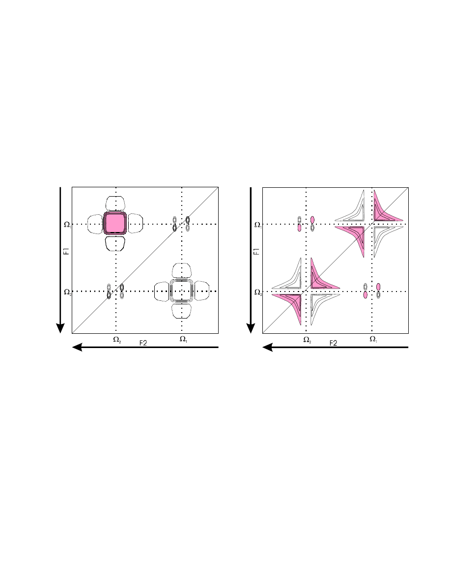
If we compare the expressions for the diagonal peak and the cross-peak, we can see that they are 90°

out of phase relativ to each other in both dimensions. E.g., for the diagonal peak we have an I

x

component which is dispersive in F1 and F2, while from the cross-peak we get an I

x

component that

is absorptive (and vice versa for the I

y

components). So, no matter what phase correction we choose

in each of the two (independently phase corrected) dimensions, always one of the two signals will be

dispersive.

Two ways of phase correcting a 2D COSY spectrum: diagonal peaks in-phase absorptive, cross-

peaks antiphase dispersive (left); or diagonal peaks in-phase dispersive, cross-peaks antiphase

absorptive (right).

No matter what phase corrrection is chosen, the dispersive tails always tend to obscure near-by

cross-peaks. Absolute value processing is no real solution either, since now the dispersive

components of both the diagonal and the cross-peaks contribute to the spectrum. Only the

employment of apodization functions with rigorous resolution enhancement and line narrowing

characteristics can yield a reasonable spectrum (although at the cost of losing S/N).