
0-8493-????-?/00/$0.00+$.50
© 2000 by CRC Press LLC
© 2001 by CRC Press LLC
10
A Taste of Probability Theory*
10.1 Introduction
In addition to its everyday use in all aspects of our public, personal, and lei-
sure lives, probability plays an important role in electrical engineering prac-
tice in at least three important aspects. It is the mathematical tool to deal with
three broad areas:
1.
The problems associated with the inherent uncertainty in the input of
certain systems.
The random arrival time of certain inputs to a
system cannot be predetermined; for example, the log-on and the
log-off times of terminals and workstations connected to a com-
puter network, or the data packets’ arrival time to a computer
network node.
2.
The problems associated with the distortion of a signal due to noise.
The
effects of noise have to be dealt with satisfactorily at each stage of
a communication system from the generation, to the transmission,
to the detection phases. The source of this noise may be due to
either fluctuations inherent in the physics of the problem (e.g.,
quantum effects and thermal effects) or due to random distortions
due to externally generated uncontrollable parameters (e.g.,
weather, geography, etc.).
3.
The problems associated with inherent human and computing machine
limitations while solving very complex systems.
Individual treatment
of the dynamics of very large number of molecules in a material,
in which more than 10
22
molecules may exist in a quart-size con-
tainer, is not possible at this time, and we have to rely on statistical
averages when describing the behavior of such systems. This is the
field of statistical physics and thermodynamics.
Furthermore, probability theory provides the necessary mathematical tools
for error analysis in all experimental sciences. It permits estimation of the

© 2001 by CRC Press LLC
error bars and the confidence level for any experimentally obtained result,
through a methodical analysis and reduction of the raw data.
In future courses in probability, random variables, stochastic processes
(which is random variables theory with time as a parameter), information
theory, and statistical physics, you will study techniques and solutions to the
different types of problems from the above list. In this very brief introduction
to the subject, we introduce only the very fundamental ideas and results —
where more advanced courses seem to almost always start.
10.2 Basics
Probability theory is best developed mathematically based on a set of axioms
from which a well-defined deductive theory can be constructed. This is
referred to as the axiomatic approach. We concentrate, in this section, on
developing the basics of probability theory, using a physical description of
the underlying concepts of probability and related simple examples, to lead
us intuitively to what is usually the starting point of the set theoretic axiom-
atic approach.
Assume that we conduct
n
independent trials under identical conditions,
in each of which, depending on chance, a particular event
A
of particular
interest either occurs or does not occur. Let
n
(
A
) be the number of experi-
ments in which
A
occurs. Then, the ratio
n
(
A
)/
n
, called the relative frequency
of the event
A
to occur in a series of experiments, clusters for
n
→
∞
about
some constant. This constant is called the probability of the event
A
, and is
denoted by:
(10.1)
From this definition, we know specifically what is meant by the statement
that the probability for obtaining a head in the flip of a fair coin is 1/2.
Let us consider the rolling of a single die as our prototype experiment :
1. The possible outcomes of this experiment are elements belonging
to the set:
(10.2)
If the die is fair, the probability for each of the elementary elements
of this set to occur in the roll of a die is equal to:
(10.3)
P A
n A
n
n
( )
lim
( )
=
→∞
S
=
{
}
1 2 3 4 5 6
, , , , ,
P
P
P
P
P
P
( )
( )
( )
( )
( )
( )
1
2
3
4
5
6
1
6
=
=
=
=
=
=

© 2001 by CRC Press LLC
2. The observer may be interested not only in the elementary elements
occurrence, but in finding the probability of a certain event which
may consist of a set of elementary outcomes; for example:
a. An event may consist of “obtaining an even number of spots on
the upward face of a randomly rolled die.” This event then
consists of all successful trials having as experimental outcomes
any member of the set:
(10.4)
b. Another event may consist of “obtaining three or more spots”
(hence, we will use this form of abbreviated statement, and not
keep repeating: on the upward face of a randomly rolled die).
Then, this event consists of all successful trials having experi-
mental outcomes any member of the set:
(10.5)
Note that, in general, events may have overlapping elementary
elements.
For a fair die, using the definition of the probability as the limit of a relative
frequency, it is possible to conclude, based on experimental trials, that:
(10.6)
while
(10.7)
and
(10.8)
The last equation [Eq. (10.8)] is the mathematical expression for the statement
that the probability of the event that includes all possible elementary out-
comes is 1 (i.e., certainty).
It should be noted that if we define the events
O
and
C
to mean the events
of “obtaining an odd number” and “obtaining a number smaller than 3,”
respectively, we can obtain these events’ probabilities by enumerating the
elements of the subsets of
S
that represent these events; namely:
(10.9)
E
= { , , }
2 4 6
B
= { , , , }
3 4 5 6
P E
P
P
P
( )
( )
( )
( )
=
+
+
=
2
4
6
1
2
P B
P
P
P
P
( )
( )
( )
( )
( )
=
+
+
+
=
3
4
5
6
2
3
P S
( )
= 1
P O
P
P
P
( )
( )
( )
( )
=
+
+
=
1
3
5
1
2

© 2001 by CRC Press LLC
(10.10)
However, we also could have obtained these same results by noting that the
events
E
and
O
(
B
and
C
) are disjoint and that their union spanned the set
S
.
Therefore, the probabilities for events
O
and
C
could have been deduced, as
well, through the relations:
P
(
O
) = 1 –
P
(
E
)
(10.11)
P
(
C
) = 1 –
P
(
B
)
(10.12)
From the above and similar observations, it would be a satisfactory repre-
sentation of the physical world if the above results were codified and ele-
vated to the status of axioms for a formal theory of probability. However, the
question becomes how many of these basic results (the axioms) one really
needs to assume, such that it will be possible to derive all other results of the
theory from this seed. This is the starting point for the formal approach to the
probability theory.
The following axioms were proven to be a satisfactory starting point.
Assign to each event
A
, consisting of elementary occurrences from the set
S
,
a number
P
(
A
), which is designated as the probability of the event
A
, and
such that:
1.
0
≤
P
(
A
)
(10.13)
2.
P(S) = 1
(10.14)
3.
If:
A
∩
B
=
∅
, where
∅
is the empty set
(10.15)
Then:
P
(
A
∪
B
) =
P
(
A
) +
P
(
B
)
In the following examples, we illustrate some common techniques for find-
ing the probabilities for certain events. Look around, and you will find
plenty more.
Example 10.1
Find the probability for getting three sixes in a roll of three dice.
Solution:
First, compute the number of elements in the total sample space.
We can describe each roll of the dice by a 3-tuplet (
a, b, c
), where
a, b,
and
c
can take the values 1, 2, 3, 4, 5, 6. There are 6
3
= 216 possible 3-tuplets. The
event that we are seeking is realized only in the single elementary occurrence
when the 3-tuplet (6, 6, 6) is obtained; therefore, the probability for this event,
for fair dice, is
P C
P
P
( )
( )
( )
=
+
=
1
2
1
3

© 2001 by CRC Press LLC
Example 10.2
Find the probability of getting only two sixes in a roll of three dice.
Solution:
The event in this case consists of all elementary occurrences having
the following forms:
(
a
, 6, 6), (6,
b,
6), (6, 6,
c
)
where
a
= 1, …, 5;
b
= 1, …, 5; and
c
= 1, …, 5. Therefore, the event
A
consists
of elements corresponding to 15 elementary occurrences, and its probability is
Example 10.3
Find the probability that, if three individuals are asked to guess a number
from 1 to 10, their guesses will be different numbers.
Solution:
There are 1000 distinct equiprobable 3-tuplets (
a, b, c
), where each
component of the 3-tuplet can have any value from 1 to 10. The event
A
occurs when all components have unequal values. Therefore, while
a
can
have any of 10 possible values,
b
can have only 9, and
c
can have only 8.
Therefore,
n
(
A
) = 8
×
9
×
10, and the probability for the event
A
is
Example 10.4
An inspector checks a batch of 100 microprocessors, 5 of which are defective.
He examines ten items selected at random. If none of the ten items is defec-
tive, he accepts the batch. What is the probability that he will accept the batch?
Solution:
The number of ways of selecting 10 items from a batch of 100 items is:
where
is the binomial coefficient and represents the number of combina-
tions of
n
objects taken
k
at a time without regard to order. It is equal to
All these combinations are equally probable.
P A
( )
=
1
216
P A
( )
=
15
216
P A
( )
.
= × ×
=
8 9 10
1000
0 72
N
C
=
−
=
=
100
10 100 10
100
10 90
10
100
!
!(
)!
!
!
!
C
k
n
n
k n k
!
!
!
.
−
(
)

© 2001 by CRC Press LLC
If the event
A
is that where the batch is accepted by the inspector, then
A
occurs when all ten items selected belong to the set of acceptable quality
units. The number of elements in
A
is
and the probability for the event
A
is
In-Class Exercises
Pb. 10.1
A cube whose faces are colored is split into 125 smaller cubes of
equal size.
a.
Find the probability that a cube drawn at random from the batch
of randomly mixed smaller cubes will have three colored faces.
b.
Find the probability that a cube drawn from this batch will have
two colored faces.
Pb. 10.2
An urn has three blue balls and six red balls. One ball was ran-
domly drawn from the urn and then a second ball, which was blue. What is
the probability that the first ball drawn was blue?
Pb. 10.3
Find the probability that the last two digits of the cube of a random
integer are 1. Solve the problem analytically, and then compare your result to
a numerical experiment that you will conduct and where you compute the
cubes of all numbers from 1 to 1000.
Pb. 10.4
From a lot of
n
resistors,
p
are defective. Find the probability that
k
resistors out of a sample of
m
selected at random are found defective.
Pb. 10.5
Three cards are drawn from a deck of cards.
a.
Find the probability that these cards are the Ace, the King, and the
Queen of Hearts.
b.
Would the answer change if the statement of the problem was “an
Ace, a King, and a Queen”?
Pb. 10.6
Show that:
where
, the complement of A, are all events in S having no element in com-
mon with A.
N A
C
( )
!
!
!
=
=
95
10 85
10
95
P A
C
C
( )
.
=
=
×
×
×
×
×
×
×
×
=
10
95
10
100
86 87 88 89 90
96 97 98 99 100
0 5837
P A
P A
( )
( )
= −
1
A

© 2001 by CRC Press LLC
NOTE
In solving certain category of probability problems, it is often conve-
nient to solve for P(A) by computing the probability of its complement and
then applying the above relation.
Pb. 10.7
Show that if A
1
, A
2
, …, A
n
are mutually exclusive events, then:
(Hint: Use mathematical induction and Eq. (10.15).)
10.3 Addition Laws for Probabilities
We start by reminding the reader of the key results of elementary set theory:
• The Commutative law states that:
(10.16)
(10.17)
• The Distributive laws are written as:
(10.18)
(10.19)
• The Associative laws are written as:
(10.20)
(10.21)
• De Morgan’s laws are
(10.22)
(10.23)
P A
A
A
P A
P A
P A
n
n
(
)
(
)
(
)
(
)
1
2
1
2
∪
∪…∪
=
+
+…+
A
B
B
A
∩ = ∩
A
B
B
A
∪ = ∪
A
B
C
A
B
A
C
∩ ∪
=
∩ ∪
∩
(
) (
)
(
)
A
B
C
A
B
A
C
∪ ∩
=
∪ ∩
∪
(
) (
)
(
)
(
)
(
)
A
B
C
A
B
C
A
B
C
∪ ∪ = ∪ ∪
= ∪ ∪
(
)
(
)
A
B
C
A
B
C
A
B
C
∩ ∩ = ∩ ∩
= ∩ ∩
(
)
A
B
A
B
∪
= ∩
(
)
A
B
A
B
∩
= ∪

© 2001 by CRC Press LLC
• The Duality principle states that: If in an identity, we replace unions
by intersections, intersections by unions, S by
∅, and ∅ by S, then
the identity is preserved.
THEOREM 1
If we define the difference of two events A
1
– A
2
to mean the events in which
A
1
occurs but not A
2
, the following equalities are valid:
(10.24)
(10.25)
(10.26)
PROOF
From the basic set theory algebra results, we can deduce the follow-
ing equalities:
(10.27)
(10.28)
(10.29)
Further note that the events (A
1
– A
2
), (A
2
– A
1
), and (A
1
∩ A
2
) are mutually
exclusive. Using the results from Pb. 10.7, Eqs. (10.27) and (10.28), and the
preceding comment, we can write:
(10.30)
(10.31)
which establish Eqs. (10.24) and (10.25). Next, consider Eq. (10.29); because of
the mutual exclusivity of each event represented by each of the parenthesis
on its LHS, we can use the results of Pb. 10.7, to write:
(10.32)
using Eqs. (10.30) and (10.31), this can be reduced to Eq. (10.26).
THEOREM 2
Given any n events A
1
, A
2
, …, A
n
and defining P
1
, P
2
, P
3
, …, P
n
to mean:
P A
A
P A
P A
A
(
)
(
)
(
)
1
2
1
1
2
−
=
−
∩
P A
A
P A
P A
A
(
)
(
)
(
)
2
1
2
1
2
−
=
−
∩
P A
A
P A
P A
P A
A
(
)
(
)
(
)
(
)
1
2
1
2
1
2
∪
=
+
−
∩
A
A
A
A
A
1
1
2
1
2
=
−
∪
∩
(
)
(
)
A
A
A
A
A
2
2
1
1
2
=
−
∪
∩
(
)
(
)
A
A
A
A
A
A
A
A
1
2
1
2
2
1
1
2
∪
=
−
∪
−
∪
∩
(
)
(
)
(
)
P A
P A
A
P A
A
(
)
(
)
(
)
1
1
2
1
2
=
−
+
∩
P A
P A
A
P A
A
(
)
(
)
(
)
2
2
1
1
2
=
−
+
∩
P A
A
P A
A
P A
A
P A
A
(
)
(
)
(
)
(
)
1
2
1
2
2
1
1
2
∪
=
−
+
−
+
∩

© 2001 by CRC Press LLC
(10.33)
(10.34)
(10.35)
etc. …, then:
(10.36)
This theorem can be proven by mathematical induction (we do not give the
details of this proof here).
Example 10.5
Using the events E, O, B, C as defined in Section 10.1, use Eq. (10.36) to show
that: P(E
∪ O ∪ B ∪ C) = 1.
Solution:
Using Eq. (10.36), we can write:
Example 10.6
Show that for any n events A
1
, A
2
, …, A
n
, the following inequality holds:
Solution:
We prove this result by mathematical induction:
P
P A
i
i
n
1
1
=
=
∑
(
)
P
P A
A
i
j
i j n
2
1
=
∩
≤ < ≤
∑
(
)
P
P A
A
A
i
j
k
i j k n
3
1
=
∩
∩
≤ < < ≤
∑
(
)
P
A
P
P
P
P
P
k
k
n
n
n
=
−
=
−
+
−
+…+ −
1
1
2
3
4
1
1
U
(
)
P E
O
B
C
P E
P O
P B
P C
P E
O
P E
B
P E
C
P O
B
P O
C
P B
C
P E
O
B
P E
O
C
P E
B
C
P O
B
C
P E
O
(
)
( )
( )
( )
( )
[ (
)
(
)
(
)
(
)
(
)
(
)]
[ (
)
(
)
(
)
(
)]
(
∪ ∪ ∪
=
+
+
+
−
∩
+
∩
+
∩
+
∩
+
∩
+
∩
+
∩ ∩
+
∩ ∩
+
∩ ∩
+
∩ ∩
−
∩ ∩ BB C
∩
=
+ + +
−
+ + + + +
+ + + + −
=
)
[
] [ ]
1
2
1
2
2
3
1
3
0
2
6
1
6
2
6
1
6
0
0 0 0 0
0
1
P
A
P A
k
k
n
k
k
n
=
=
≤
∑
1
1
U
(
)

© 2001 by CRC Press LLC
• For n = 2, the result holds because by Eq. (10.26) we have:
and since any probability is a non-negative number, this leads to
the inequality:
• Assume that the theorem is true for (n – 1) events, then we can write:
• Using associativity, Eq. (10.26), the result for (n – 1) events, and the
non-negativity of the probability, we can write:
which is the desired result.
In-Class Exercises
Pb. 10.8
Show that if the events A
1
, A
2
, …, A
n
are such that:
then:
Pb. 10.9
Show that if the events A
1
, A
2
, …, A
n
are such that:
P A
A
P A
P A
P A
A
(
)
(
)
(
)
(
)
1
2
1
2
1
2
∪
=
+
−
∩
P A
A
P A
P A
(
)
(
)
(
)
1
2
1
2
∪
≤
+
P
A
P A
k
k
n
k
k
n
=
=
≤
∑
2
2
U
(
)
P
A
P A
A
P A
P
A
P A
A
P A
P A
P A
A
k
k
n
k
k
n
k
k
n
k
k
n
k
k
n
k
k
n
=
=
=
=
=
=
=
∪
=
+
−
∩
≤
( )
+
−
∩
∑
1
1
1
1
2
1
2
1
2
1
2
U
U
U
U
U
(
)
(
)
≤
=
∑
P A
k
k
n
(
)
1
A
A
A
n
1
2
⊂
⊂ … ⊂
P
A
P A
k
k
n
n
=
=
1
U
(
)
A
A
A
n
1
2
⊃ ⊃
… ⊃

© 2001 by CRC Press LLC
then:
Pb. 10.10
Find the probability that a positive integer randomly selected will
be non-divisible by:
a.
2 and 3.
b.
2 or 3.
Pb. 10.11
Show that the expression for Eq. (10.36) simplifies to:
when the probability for the intersection of any number of events is indepen-
dent of the indices.
Pb. 10.12
A filing stack has n drawers, and a secretary randomly files m-let-
ters in these drawers.
a.
Assuming that m > n, find the probability that there will be at least
one letter in each drawer.
b.
Plot this probability for n = 12, and 15
≤ m ≤ 50.
(Hint: Take the event A
j
to mean that no letter is filed in the j
th
drawer and
use the result of Pb. 10.11.)
10.4 Conditional Probability
The conditional probability of an event A assuming C and denoted by
is, by definition, the ratio:
(10.37)
Example 10.7
Considering the events E, O, B, C as defined in Section 10.2 and the above def-
inition for conditional probability, find the probability that the number of
spots showing on the die is even, assuming that it is equal to or greater than 3.
P
A
P A
k
k
n
n
=
=
1
I
(
)
P A
A
A
C P A
C P A
A
C P A
A
A
P A
A
A
n
n
n
n
n
n
(
)
(
)
(
)
(
)
(
)
(
)
1
2
1
1
2
1
2
3
1
2
3
1
1
2
1
∪
∪…∪
=
−
∩
+
∩
∩
−
…+ −
∩
∩…∩
−
P A C
(
)
P A C
P A
C
P C
(
)
(
)
( )
=
∩

© 2001 by CRC Press LLC
Solution:
In the above notation, we are asked to find the quantity
Using Eq. (10.37), this is equal to:
In this case,
When this happens, we say that the two events E
and B are independent.
Example 10.8
Find the probability that the number of spots showing on the die is even,
assuming that it is larger than 3.
Solution:
Call D the event of having the number of spots larger than 3. Using
Eq. (10.37),
is equal to:
In this case,
and thus the two events E and D are not
independent.
Example 10.9
Find the probability of picking a blue ball first, then a red ball from an urn
that contains five red balls and four blue balls.
Solution:
From the definition of conditional probability [Eq. (10.37)], we can
write:
The probability of picking a blue ball first is
The conditional probability is given by:
P E B
(
).
P E B
P E
B
P B
P
P
(
)
(
)
( )
({ , })
({ , , , })
=
∩
=
=
=
4 6
3 4 5 6
2
6
4
6
1
2
P E B
P E
(
)
( ).
=
P E D
(
)
P E D
P E
D
P D
P
P
(
)
(
)
( )
({ , })
({ , , })
=
∩
=
=
=
4 6
4 5 6
2
6
3
6
2
3
P E D
P E
(
)
( );
≠
P
P
P
(
(
(
Blue ball first and Red ball second) =
Red ball second Blue ball first)
Blue ball first)
×
P Blue ball first
Original number of Blue balls
Total number of balls
(
)
=
=
4
9

© 2001 by CRC Press LLC
giving:
10.4.1 Total Probability and Bayes Theorems
TOTAL PROBABILITY THEOREM
If [A
1
, A
2
, …, A
n
] is a partition of the total elementary occurrences set S, that is,
and B is an arbitrary event, then:
(10.38)
PROOF
From the algebra of sets, and the definition of a partition, we can
write the following equalities:
(10.39)
Since the events
and are mutually exclusive for i
≠ j,
then using the results of Pb. 10.7, we can deduce that:
(10.40)
Now, using the conditional probability definition [Eq. (10.38)], Eq. (10.40) can
be written as:
(10.41)
This result is known as the Total Probability theorem.
P(Red ball second Blue ball first)
Number of Red balls
Number of balls remaining after first pick
=
=
5
8
P(Blue ball first and Red ball second)
= × =
4
9
5
8
5
18
A
S
A
A
i
j
i
i
n
i
j
=
=
∩
= ∅
≠
1
U
and
for
P B
P B A P A
P B A P A
P B A P A
n
n
( )
(
) (
)
(
) (
)
(
) (
)
=
+
+…+
1
1
2
2
B
B
S
B
A
A
A
B
A
B
A
B
A
n
n
= ∩ = ∩
∪
∪…∪
=
∩
∪ ∩
∪…∪ ∩
(
)
(
)
(
)
(
)
1
2
1
2
(
)
)
B
A
B
A
i
j
∩
∩
and (
P B
P B
A
P B
A
P B
A
n
( )
(
)
(
)
(
)
=
∩
+
∩
+…+
∩
1
2
P B
P B A P A
P B A P A
P B A P A
n
n
( )
(
) (
)
(
) (
)
(
) (
)
=
+
+…+
1
1
2
2

© 2001 by CRC Press LLC
BAYES THEOREM
(10.42)
PROOF
From the definition of the conditional probability [Eq. (10.37)], we
can write:
(10.43)
Again, using Eqs. (10.37) and (10.43), we have:
(10.44)
Now, substituting Eq. (10.41) in the denominator of Eq. (10.44), we obtain Eq.
(10.42).
Example 10.10
A digital communication channel transmits the signal as a collection of ones
(1s) and zeros (0s). Assume (statistically) that 40% of the 1s and 33% of the 0s
are changed upon transmission. Suppose that, in a message, the ratio
between the transmitted 1 and the transmitted 0 was 5/3. What is the proba-
bility that the received signal is the same as the transmitted signal if:
a.
The received signal was a 1?
b.
The received signal was a 0?
Solution:
Let O be the event that 1 was received, and Z be the event that 0 was
received. If H
1
is the hypothesis that 1 was received and H
0
is the hypothesis
that 0 was received, then from the statement of the problem, we know that:
giving:
Furthermore, from the text of the problem, we know that:
P A B
P B A P A
P B A P A
P B A P A
P B A P A
i
i
i
n
n
(
)
(
) (
)
(
) (
)
(
) (
)
(
) (
)
=
+
+…+
1
1
2
2
P B
A
P A B P B
i
i
(
)
(
) ( )
∩
=
P A B
P B A P A
P B
i
i
i
(
)
(
) (
)
( )
=
P H
P H
P H
P H
(
)
(
)
(
)
(
)
1
0
1
0
5
3
1
=
+
=
and
P H
P H
(
)
(
)
1
0
5
8
3
8
=
=
and

© 2001 by CRC Press LLC
From the total probability result [Eq. (10.41)], we obtain:
and
The probability that the received signal is 1 if the transmitted signal was 1
from Bayes theorem:
Similarly, we can obtain the probability that the received signal is 0 if the
transmitted signal is 0:
In-Class Exercises
Pb. 10.13
Show that when two events A and B are independent, the addi-
tion law for probability becomes:
P O H
P Z H
P O H
P Z H
(
)
(
)
(
)
(
)
1
1
0
0
3
5
2
5
1
3
2
3
=
=
=
=
and
and
P O
P O H P H
P O H P H
( )
(
) (
)
(
) (
)
=
+
= × + × =
1
1
0
0
3
5
5
8
1
3
3
8
1
2
P Z
P Z H P H
P Z H P H
( )
(
) (
)
(
) (
)
=
+
= × + × =
1
1
0
0
2
5
5
8
2
3
3
8
1
2
P H O
P H P O H
P O
(
)
(
) (
)
( )
1
1
1
5
3
3
5
1
2
3
4
=
=
=
P H Z
P H P Z H
P Z
(
)
(
) (
)
( )
0
0
0
3
8
2
3
1
2
1
2
=
=
=
P A
B
P A
P B
P A P B
(
)
( )
( )
( ) ( )
∪
=
+
−

© 2001 by CRC Press LLC
Pb. 10.14
Consider four boxes, each containing 1000 resistors. Box 1 con-
tains 100 defective items; Box 2 contains 400 defective items; Box 3 contains
50 defective items; and Box 4 contains 80 defective items.
a.
What is the probability that a resistor chosen at random from any
of the boxes is defective?
b.
What is the probability that if the resistor is found defective, it
came from Box 2?
(Hint: The randomness in the selection of the box means that: P(B
1
) = P(B
2
)
= P(B
3
) = P(B
4
) = 0.25.)
10.5 Repeated Trials
Bernoulli trials refer to identical, successive, and independent trials, in which
an elementary event A can occur with probability:
p = P(A)
(10.45)
or fail to occur with probability:
q = 1 – p
(10.46)
In the case of n consecutive Bernoulli trials, each elementary event can be
described by a sequence of 0s and 1s, such as in the following:
(10.47)
where n is the number of trials, k is the number of successes, and (n – k) is the
number of failures. Because the trials are independent, the probability for the
above single occurrence is:
(10.48)
The total probability for the event with k successes in n trials is going to be
the probability of the single event multiplied by the number of configurations
with a given number of digits and a given number of 1s. The number of such
configurations is given by the binomial coefficient
Therefore:
ω =
…
−
1 0 0 0 1
0 1
n digits
k ones
1 2
44
3
44
P
p q
k n k
( )
ω =
−
C
k
n
.

© 2001 by CRC Press LLC
(10.49)
Example 10.11
Find the probability that the number 3 will appear twice in five independent
rolls of a die.
Solution:
In a single trial, the probability of success (i.e., 3 showing up) is
Therefore, the probability that it appears twice in five independent rolls will be
Example 10.12
Find the probability that in a roll of two dice, three occurrences of snake-eyes
(one spot on each die) are obtained in ten rolls of the two dice.
Solution:
The space S of the roll of two dice consists of 36 elementary elements
(6
× 6), only one of which results in a snake-eyes configuration; therefore:
p = 1/36; k = 3; n = 10
and
In-Class Exercises
Pb. 10.15
Assuming that a batch of manufactured components has an 80%
chance of passing an inspection, what is the chance that at least 16 batches in
a lot of 20 would pass the inspection?
Pb. 10.16
In an experiment, we keep rolling a fair die until it comes up
showing three spots. What are the probabilities that this will take:
a.
Exactly four rolls?
b.
At least four rolls?
c.
At most four rolls?
P k
n
C p q
k
n
k n k
( successes in
trials)
=
−
p
=
1
6
P
C p q
(
!
! !
.
2
5
2 3
1
6
5
6
0 16075
2
5
2 5
2
3
successes in 5 trials) =
=
=
P
C p q
(
!
! !
.
3 successes in 10 trials) =
3
10
3 7
3
7
10
3 7
1
36
35
36
0 00211
=
=

© 2001 by CRC Press LLC
Pb. 10.17
Let X be the number of successes in a Bernoulli trials experiment
with n trials and the probability of success p in each trial. If the mean number
of successes m, also called average value
and expectation value E(X), is
defined as:
and the variance is defined as:
show that:
10.5.1
Generalization of Bernoulli Trials
In the above Bernoulli trials, we considered the case of whether or not a single
event A was successful (i.e., two choices). This was the simplest partition of
the set S.
In cases where we partition the set S in r subsets: S = {A
1
, A
2
, …, A
r
}, and
the probabilities for these single events are, respectively: {p
1
, p
2
, …, p
r
}, where
p
1
+ p
2
+ … + p
r
= 1, it can be easily proven that the probability in n indepen-
dent trials for the event A
1
to occur k
1
times, the event A
2
to occur k
1
times,
etc., is given by:
(10.50)
where k
1
+ k
2
+ … + k
r
= n
Example 10.13
Consider the sum of the spots in a roll of two dice. We partition the set of out-
comes {2, 3, …, 11, 12} into the three events A
1
= {2, 3, 4, 5}, A
2
= {6, 7}, A
3
= {8,
9, 10, 11, 12}. Find P(1, 7, 2; 10).
Solution:
The probabilities for each of the events are, respectively:
X
m
X
E X
XP X
≡
≡
≡
∑
( )
( )
V X
E X
X
( )
((
) )
≡
−
2
X
np
V X
np
p
=
=
−
and
( )
(
)
1
P k k
k n
n
k k
k
p p
p
r
r
k
k
r
k
r
( ,
,
,
; )
!
! !
!
1
2
1
2
1
2
1
2
…
=
…
…
p
p
p
1
2
3
10
36
11
36
15
36
=
=
=
,
,

© 2001 by CRC Press LLC
and
10.6 The Poisson and the Normal Distributions
In this section, we obtain approximate expressions for the binomial distribu-
tion in different limits. We start by considering the expression for the proba-
bility of k successes in n Bernoulli trials with two choices for outputs; that is,
Eq. (10.49).
10.6.1
The Poisson Distribution
Consider the limit when p << 1, but np
≡ a ≈ O(1). Then:
(10.51)
But in the limit n
→ ∞,
(10.52)
giving:
(10.53)
Now consider P(k = 1); it is equal to:
(10.54)
For P(k = 2), we obtain:
(10.55)
P 1 7 2 10
10
1 7 2
10
36
11
36
15
36
0 00431
1
7
2
, , ;
!
! ! !
.
(
)
=
=
P k
n
n
p
p
a
n
n
n
(
)
!
! !
(
)
=
=
−
=
−
0
0
1
1
0
1
−
=
−
a
n
e
n
a
P k
e
a
(
)
=
=
−
0
lim (
)
!
!(
)!
(
)
n
n
n
a
P k
n
n
p
p
a
a
n
ae
→∞
−
−
= =
−
−
≈
−
≈
1
1
1
1
1
1
1
lim (
)
!
!(
)!
(
)
!
!
n
n
n
a
P k
n
n
p
p
a
a
n
a
e
→∞
−
−
=
=
−
−
≈
−
≈
2
2
2
1
2
1
2
2
2
2
2
© 2001 by CRC Press LLC
Similarly,
(10.56)
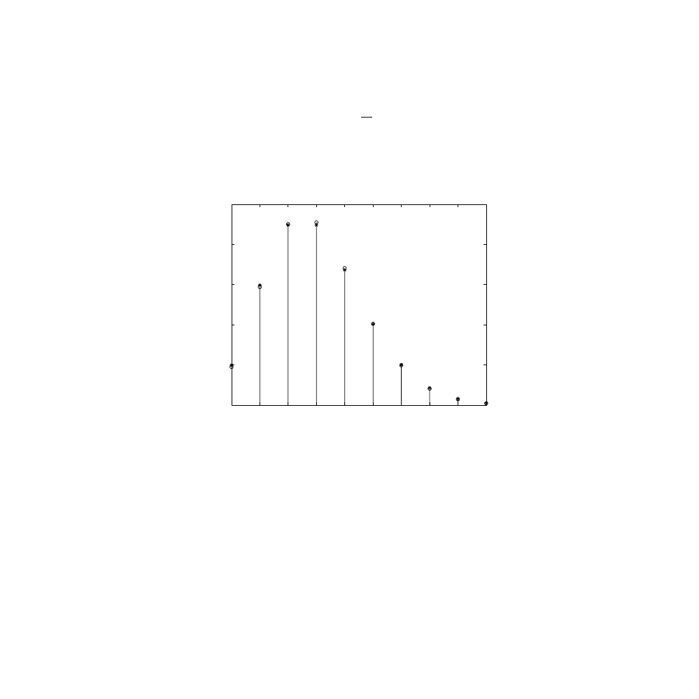
We compare in
the exact with the approximate expression for
the probability distribution, in the region of validity of the Poisson approx-
imation.
Example 10.14
A massive parallel computer system contains 1000 processors. Each proces-
sor fails independently of all others and the probability of its failure is 0.002
over a year. Find the probability that the system has no failures during one
year of operation.
Solution:
This is a problem of Bernoulli trials with n = 1000 and p = 0.002:
or, using the Poisson approximate formula, with a = np = 2:
FIGURE 10.1
The Poisson distribution.
lim ( )
!
n
k
a
P k
a
k
e
→∞
−
≈
0
1
2
3
4
5
6
7
8
9
0
0.05
0.1
0.15
0.2
0.25
k
P ( k )
Poisson Distribution : n = 100 ; p = 0.03
Stems : Exact Distribution
Asterisks : Poisson Approximation
P k
C
p
p
(
)
(
)
( .
)
.
=
=
−
=
=
0
1
0 998
0 13506
0
1000
0
1000
1000
P k
e
e
a
(
)
.
=
≈
=
≈
−
−
0
0 13533
2

© 2001 by CRC Press LLC
Example 10.15
Due to the random vibrations affecting its supporting platform, a recording
head introduces glitches on the recording medium at the rate of n = 100
glitches per minute. What is the probability that k = 3 glitches are introduced
in the recording over any interval of time
∆t = 1s?
Solution:
If we choose an interval of time equal to 1 minute, the probability
for an elementary event to occur in the subinterval
∆t in this 1 minute inter-
val is
The problem reduces to finding the probability of k = 3 in n = 100 trials.
The Poisson formula gives this probability as:
where a = 100/60. (For comparison purposes, the exact value for this proba-
bility, obtained using the binomial distribution expression, is 0.1466.)
Homework Problem
Pb. 10.18
Let A
1
, A
2
, …, A
m+1
be a partition of the set S, and let p
1
, p
2
, …, p
m+1
be the probabilities associated with each of these events. Assuming that n
Bernoulli trials are repeated, show, using Eq. (10.50), that the probability that
the event A
1
occurs k
1
times, the event A
2
occurs k
2
times, etc., is given in the
limit n
→ ∞ by:
where a
i
= np
i
.
10.6.2
The Normal Distribution
Prior to considering the derivation of the normal distribution, let us recall
Sterling’s formula, which is the approximation of n! when n
→ ∞:
(10.57)
p
=
1
60
P( )
!
exp
.
3
1
3
100
60
100
60
0 14573
3
=
−
=
lim ( ,
,
,
; )
( )
!
( )
!
(
)
!
n
m
k
a
k
a
m
k
a
m
P k k
k
n
a
e
k
a
e
k
a
e
k
m
m
→∞
+
−
−
−
…
=
…
1
2
1
1
1
2
2
1
1
2
2
lim !
n
n
n
n
n n e
→∞
−
≈ 2π

© 2001 by CRC Press LLC
We seek the approximate form of the binomial distribution in the limit of very
large n and npq >> 1. Using Eq. (10.57), the expression for the probability
given in Eq. (10.49), reduces to:
(10.58)
Now examine this expression in the neighborhood of the mean (see
Pb. 10.17
). We define the distance from this mean, normalized to the square
root of the variance, as:
(10.59)
Using the leading two terms of the power expansion of (ln(1 +
ε) = ε – ε
2
/2 +
…), the natural logarithm of the two parentheses on the RHS of Eq. (10.58)
can be approximated by:
(10.60)
(10.61)
Adding Eqs. (10.61) and (10.62), we deduce that:
(10.62)
Furthermore, we can approximate the square root term on the RHS of Eq.
(10.58) by its value at the mean; that is
(10.63)
Combining Eqs. (10.62) and (10.63), we can approximate Eq. (10.58), in this
limit, by the Gaussian distribution:
P k
n
n
k n k
np
k
nq
n k
k
n k
(
(
)
(
)
successes in
trials)
=
−
−
−
1
2
π
x
k np
npq
=
−
ln
(
)
k
np
np
npq x
q
np
x
q
np
x
k
≈ −
+
−
−
1
2
2
ln
(
)
n k
nq
nq
npq x
p
nq
x
p
nq
x
n k
−
≈ −
−
−
−
− −
(
)
1
2
2
lim
(
)
n
k
n k
x
np
k
nq
n k
e
→∞
−
−
−
=
2
n
n n k
npq
(
)
−
≈
1
© 2001 by CRC Press LLC
(10.64)
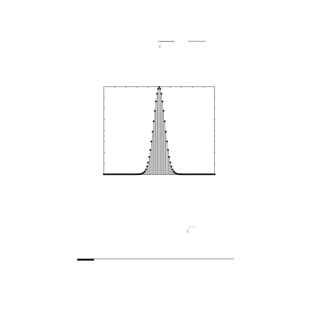
This result is known as the De Moivre-Laplace theorem. We compare in
the binomial distribution and its Gaussian approximation in the
region of the validity of the approximation.
Example 10.16
A fair die is rolled 400 times. Find the probability that an even number of
spots show up 200 times, 210 times, 220 times, and 230 times.
Solution:
In this case, n = 400; p = 0.5; np = 200; and
Using Eq. (10.65), we get:
Homework Problems
Pb. 10.19
Using the results of Pb. 4.34, relate in the region of validity of the
Gaussian approximation the quantity:
FIGURE 10.2
The normal (Gaussian) distribution.
P k
n
npq
k np
npq
(
exp
(
)
successes in
trials)
=
−
−
1
2
2
2
π
0
10
20
30
40
50
60
70
80
90
100
0
0.01
0.02
0.03
0.04
0.05
0.06
0.07
0.08
k
P ( k )
Gaussian Distribution : n = 100 ; p = 0.5
Stems : Exact Distribution
Asterisks : Gaussian Approximation
npq
= 10.
P
P
P
P
(
.
;
(
.
(
.
;
(
.
200
0 03989
210
0 02419
220
0 00540
230
4 43 10
4
even)
even)
even)
even)
=
=
=
=
×
−

© 2001 by CRC Press LLC
to the Gaussian integral, specifying each of the parameters appearing in your
expression. (Hint: First show that in this limit, the summation can be approx-
imated by an integration.)
Pb. 10.20
Let A
1
, A
2
, …, A
r
be a partition of the set S, and let p
1
, p
2
, …, p
r
be
the probabilities associated with each of these events. Assuming n Bernoulli
trials are repeated, show that, in the limit n
→ ∞ and where k
i
are in the vicin-
ity of np
i
>> 1, the following approximation is valid:
P k
n
k k
k
( successes in
trials)
=
∑
1
2
P k k
k n
k
np
np
k
np
np
n
p
p
r
r
r
r
r
r
( ,
,
,
; )
exp
(
)
(
)
(
)
1
2
1
1
2
1
2
1
1
1
2
2
…
=
−
−
+…+
−
…
−
π
Document Outline
- ELEMENTARY MATHEMATICAL and COMPUTATIONAL TOOLS for ELECTRICAL and COMPUTER ENGINEERS USING MATLAB ®
Wyszukiwarka
Podobne podstrony:
1080 PDF C09
1080 PDF C07
1080 PDF C08
1080 PDF ADDE
1080 PDF C04
1080 PDF C06
1080 PDF C03
1080 PDF TOC
1080 PDF C01
1080 PDF C05
1080 PDF C02
1080 PDF REF
1080 PDF C09
1080 PDF C07
1080 PDF C08
instr 2011 pdf, Roztw Spektrofoto
(ebook PDF)Shannon A Mathematical Theory Of Communication RXK2WIS2ZEJTDZ75G7VI3OC6ZO2P57GO3E27QNQ
KSIĄŻKA OBIEKTU pdf
zsf w3 pdf
więcej podobnych podstron