0-8493-????-?/00/$0.00+$.50
© 2000 by CRC Press LLC

Difference Equations

This chapter introduces difference equations and examines some simple but
important cases of their applications. We develop simple algorithms for their
numerical solutions and apply these techniques to the solution of some prob-
lems of interest to the engineering professional. In particular, it illustrates
each type of difference equation that is of widespread interest.

2.1

Simple Linear Forms

The following components are needed to define and solve a difference
equation:

1. An ordered array defining an index for the sequence of elements
2. An equation connecting the value of an element having a certain

index with the values of some of the elements having lower indices
(the order of the equation being defined by the number of lower
indices terms appearing in the difference equation)

3. A sufficient number of the values of the elements at the lowest

indices to act as seeds in the recursive generation of the higher
indexed elements.

For example, the Fibonacci numbers are defined as follows:

1. The ordered array is the set of positive integers
2. The defining difference equation is of second order and is given by:

(

+ 2) =

(

+ 1) +

(

)

(2.1)

3. The initial conditions are

(1) =

(2) = 1 (note that the required

number of initial conditions should be the same as the order of the
equation).

From the above, it is then straightforward to compute the first few

Fibonacci numbers:

1, 1, 2, 3, 5, 8, 13, 21, 34, 55, 89, …

Example 2.1

Write a program for finding the first 20 Fibonacci numbers.

Solution:

The following program fulfills this task:

N=18;

F(1)=1;

F(2)=1;

for k=1:N

F(k+2)=F(k)+F(k+1);

end

It should be noted that the value of the different elements of the sequence
depends on the values of the initial conditions, as illustrated in

Pb. 2.1

, which

follows.

In-Class Exercises

Pb. 2.1

Find the first 20 elements of the sequence that obeys the same recur-

sion relation as that of the Fibonacci numbers, but with the following initial
conditions:

(1) = 0.5 and

(2) = 1

Pb. 2.2

Find the first 20 elements of the sequence generated by the follow-

ing difference equation:

(

+ 3) =

(

) +

(

+ 1) +

(

+ 2)

with the following boundary conditions:

(1) = 1,

(2) = 2, and

(3) = 3

Why do we need to specify three initial conditions?

2.2

Amortization

In this application of difference equations, we examine simple problems of
finance that are of major importance to every engineer, on both the personal
and professional levels. When the purchase of any capital equipment or real
estate is made on credit, the assumed debt is normally paid for by means of
a process known as amortization. Under this plan, a debt is repaid in a
sequence of periodic payments where a portion of each payment reduces the
outstanding principal, while the remaining portion is for interest on the loan.

Suppose that the original debt to be paid is

and that interest charges are

compounded at the rate

per payment period. Let

(

) be the outstanding

principal after the

payment, and

(

) the amount of the

payment.

After the

payment period, the outstanding debt increased by the inter-

est due on the previous principal

(

– 1), and decreased by the amount of

payment

(

), this relation can be written in the following difference equa-

tion form:

(

) = (1 +

)

(

–1) –

(

)

(2.2)

We can simplify the problem and assume here that the bank wants its

money back in equal amounts over

periods (this can be in days, weeks,

months, or years; note, however, that whatever unit is used here should be
the same as used for the assignment of the value of the interest rate

). There-

fore, let

(

) =

for

= 1, 2, 3, …,

(2.3)

Now, using Eq. (2.2), let us iterate the first few terms of the difference
equation:

(1) = (1 +

)

(0) –

= (1 +

)

–

(2.4)

Since

is the original capital borrowed;

= 2, using Eq. (2.2) and Eq. (2.4), we obtain:

(2) = (1 +

)

(1) –

= (1 +

)

–

(1 +

) –

(2.5)

= 3, using Eq. (2.2), (2.4), and (2.5), we obtain:

(3) = (1 +

)

(2) –

= (1 +

)

–

(1 +

)

–

(1 +

) –

(2.6)

etc. …

and for an arbitrary

, we can write, by induction, the general expression:

(2.7)

Using the expression for the sum of a geometric series, from the appendix, the
expression for

(

) then reduces to:

(2.8)

, the debt is paid off and the bank is owed no further payment;

therefore:

(2.9)

From this equation, we can determine the amount of each of the (equal)
payments:

(2.10)

Question:

What percentage of the first payment is going into retiring the

principal?

In-Class Exercises

Pb. 2.3

Given the principal, the number of periods and the interest rate, use

Eq. (2.10) to write a MATLAB program to find the amount of payment per
period, assuming the payment per period is the same for all periods.

Pb. 2.4

Use the same reasoning as for the amortization problem to write the

difference equation for an individual’s savings plan. Let

(

) be the savings

balance on the first day of the

year and

(

) the amount of deposit made

in the

year.

Write a MATLAB program to compute

(

) if the sequence

(

) and the inter-

est rate

are given. Specialize to the case where you deposit an amount that

increases by the rate of inflation

. Compute and plot the total value of the

savings as a function of

if the deposit in the first year is $1000, the yearly

interest rate is 6%, and the yearly rate of inflation is 3%. (

Hint:

For simplicity,

assume that the deposits are made on December 31 of each year, and that the
balance statement is issued on January 1 of each year.)

y k

r C p

( ) (

)

(

)

= +

−

∑

y k

r C p

( ) (

)

(

)

= +

−







y N

C p

( )

(

)

(

)

= = +

−







−

(

)

(

)

2.3

An Iterative Geometric Construct: The Koch Curve

In your previous studies of 2-D geometry, you encountered classical geomet-
ric objects such as the circle, the triangle, the square, different polygons, etc.
These shapes only approximate the shapes that you observe in nature (e.g.,
the shapes of clouds, mountain ranges, rivers, coastlines, etc.). In a successful
effort to address the limitations of classical geometry, mathematicians have
developed, over the last century and more intensely over the last three
decades, a new geometry called fractal geometry. This geometry defines the
geometrical object through an iterative transformation applied an infinite
number of times on an initial simple geometrical object. We illustrate this
new concept in geometry by considering the Koch curve (see

Figure 2.1

The Koch curve has the following simple geometrical construction. Begin

with a straight line of length

. This initial object is called the initiator. Now

partition it into three equal parts. Then replace the middle line segment by an
equilateral triangle (the segment you removed is its base). This completes the
basic construction, which transformed the line segment into four non-colin-
ear smaller parts. This constructional prescription is called the generator. We
now repeat the transformation, taking each of the resulting line segments,
partitioning them into three equal parts, removing the middle section, etc.

FIGURE 2.1

The first few steps in the construction of the Koch curve.

This process is repeated indefinitely.

Figure 2.1

the first two steps of this con-

struction. It is interesting to observe that the Koch curve is an example of a
curve where there is no way to fit a tangent to any of its points. In a sense, it
is an example of a curve that is made out of corners everywhere.

The detailed study of these objects is covered in courses in fractal geometry,

chaos, dynamic systems, etc. We limit ourselves here to the simple problems
of determining the number of segments, the length of each segment, the
length of the curve, and the area bounded by the curve and the horizontal
axis, following the

step:

1. After the first step, we are left with a curve made up of four line

segments of equal length; after the second step, we have (4

segments; and the number of segments after

steps, is

(

k) = 4

(2.11)

2. If the initiator had length L, the length of the segment after the first

step is L/3, L/(3)

, after the second step and after k steps:

s(k) = L/(3)

(2.12)

3. Combining the results of Eqs. (2.11) and (2.12), we deduce that the

length of the curve after k steps:

(2.13)

4. The number of vertices in this curve, denoted by u(k), is equal to

the number of segments plus one:

u(k) = 4

+ 1

(2.14)

5. The area enclosed by the Koch curve and the horizontal line can be

deduced from solving a difference equation: the area enclosed after
the k

step is equal to the area enclosed in the (k – 1)

step plus the

number of the added triangles multiplied by their individual area:

Number of new triangles =

(2.15)

Area of the new equilateral triangle =

(2.16)

P k

( )

= × 





4
3

u k

( )

(

)

−









1
3

s k

( )









from which the difference equation for the area can be deduced:

(2.17)

The initial condition for this difference equation is:

(2.18)

Clearly, the solution of the above difference equation is the sum of a geo-

metric series, and can therefore be written analytically. For k

→ ∞, this area

has the limit:

(2.19)

However, if you did not notice the relationship of the above difference

equation with the sum of a geometric series, you can still solve this equation
numerically, using the following routine and assuming L = 1:

N=25;

A=zeros(N,1); %preallocating size of array speeds

% computation

m=1:N;

A(1)=(sqrt(3)/24)*(2/3);

for k=2:N

A(k)=A(k-1)+(sqrt(3)/24)*((2/3)^(2*k-1));

end

stem(m,A,'*')

The above plot shows the value of the area on the first 20 iterations of the
function, and as can be verified, the numerical limit of this area has the same
value as the analytical expression given in Eq. (2.19).

Before leaving the Koch curve, we note that although the area of the curve

goes to a finite limit as the index increases, the value of the length of the curve
[Eq. (2.13)] continues to increase. This is a feature not encountered in the clas-
sical geometric objects with which you are most familiar.

A k

u k

A k

( )

(

)

( )

(

)

(

)

− +

−







− +









−

4 3

2
3

( )

4 9

A k

(

)

→ ∞ =

In-Class Exercise

Pb. 2.5

Write a program to draw the Koch curve at the k

step. (Hint: Start-

ing with the farthest left vertex and going clockwise, write a difference equa-
tion relating the coordinates of a vertex with those of the preceding vertex,
the length of the segment, and the angle that the line connecting the two con-
secutive vertices makes with the x-axis.)

2.4

Solution of Linear Constant Coefficients Difference
Equations

In Section 2.1, we explored the general numerical techniques for solving dif-
ference equations. In this section, we consider, some special techniques for
obtaining the analytical solutions for the class of linear constant coefficients
difference equations. The related physical problem is to determine, for a lin-
ear system, the output y(k), k > 0, given a specific input u(k) and a specific set
of initial conditions. We discuss, at this stage, the so-called direct method.

The general expression for this class of difference equation is given by:

(2.20)

The direct method assumes that the total solution of a linear difference equa-
tion is the sum of two parts — the homogeneous solution and the particular
solution:

y(k) = y

homog.

(k) + y

partic.

(k)

(2.21)

The homogeneous solution is independent of the input u(k), and the RHS of
the difference equation is equated to zero; that is,

(2.22)

2.4.1

Homogeneous Solution

Assume that the solution is of the form:

a y k

b u k

(

)

(

)

− =

−

∑

a y k

(

)

− =

∑

homog.

(k) =

(2.23)

Substituting in the homogeneous equation, we obtain the following algebraic
equation:

(2.24)

(2.25)

The polynomial in parentheses is called the characteristic polynomial of the
system. The roots can be obtained analytically for all polynomials up to order
4; otherwise, they are obtained numerically. In MATLAB, they can be
obtained graphically when they are all real, or through the roots command
in the most general case. We introduce this command in Chapter 5. In all the
following examples in this chapter, we restrict ourselves to cases for which
the roots can be obtained analytically.

If we assume that the roots are all distinct, the general solution to the homo-

geneous difference equation is:

(2.26)

where

, …,

are the roots of the characteristic polynomial.

Example 2.2

Find the homogeneous solution of the difference equation

y(k) – 3y(k – 1) – 4y(k – 2) = 0

Solution:

The characteristic polynomial associated with this equation leads

to the quadratic equation:

– 3

λ – 4 = 0

The roots of this equation are –1 and 4, respectively. Therefore, the solution of
the homogeneous equation is:

homog.

(k) = C

(–1)

+ C

(4)

The constants C

and C

are determined from the initial conditions y(1) and

y(2). Substituting, we obtain:

k j

−

∑

k N

−

+…+

(

)

homog.

( )

+…+

1 1

NOTE

If the characteristic polynomial has roots of multiplicity m, then the

portion of the homogeneous solution corresponding to that root can be writ-
ten, instead of C

, as:

In-Class Exercises

Pb. 2.6

Find the homogeneous solution of the following second-order dif-

ference equation:

y(k) = 3y(k – 1) – 2y(k – 2)

with the initial conditions: y(0) = 1 and y(1) = 2. Then check your results
numerically.

Pb. 2.7

Find the homogeneous solution of the following second-order dif-

ference equation:

y(k) = [2 cos(

θ)]y(k – 1) – y(k – 2)

with the initial conditions: y(–2) = 0 and y(–1) = 1. Check your results
numerically.

2.4.2

Particular Solution

The particular solution depends on the form of the input signal. The follow-
ing table summarizes the form of the particular solution of a linear equation
for some simple input functions:

For more complicated input signals, the z-transform technique provides the
simplest solution method. This technique is discussed in great detail in
courses on linear systems.

Input Signal

Particular Solution

A (constant)

B (constant)

+ B

M–1

+ … + B

{A cos(

k), A sin(

k)}

cos(

k) + B

sin(

4
5

= −

( )

and

C k

( )

+…+

−

In-Class Exercise

Pb. 2.8

Find the particular solution of the following second-order difference

equation:

y(k) – 3y(k – 1) + 2y(k – 2) = (3)

for k > 0

2.4.3

General Solution

The general solution of a linear difference equation is the sum of its homoge-
neous solution and its particular solution, with the constants adjusted, so as
to satisfy the initial conditions. We illustrate this general prescription with an
example.

Example 2.3

Find the complete solution of the first-order difference equation:

y(k + 1) + y(k) = k

with the initial condition y(0) = 0.

Solution:

First, solve the homogeneous equation y(k + 1) + y(k) = 0. The char-

acteristic polynomial is

λ + 1 = 0; therefore,

homog.

= C(–1)

The particular solution can be obtained from the above table. Noting that the
input signal has the functional form k

, with M = 1, then the particular solu-

tion is of the form:

partic.

= B

k + B

(2.27)

Substituting back into the original equation, and grouping the different pow-
ers of k, we deduce that:

= 1/2 and B

= –1/4

The complete solution of the difference equation is then:

y k

( )

(

)

= −

−

The constant C is determined from the initial condition:

giving for the constant C the value 1/4.

In-Class Exercises

Pb. 2.9

Use the following program to model Example 2.3:

N=19;

y(1)=0;

for k=1:N

y(k+1)=k-y(k);

end

Verify the closed-form answer.

Pb. 2.10

Find, for k

≥ 2, the general solution of the second-order difference

equation:

y(k) – 3y(k – 1) – 4y(k – 2) = 4

+ 2

× 4

k–1

with the initial conditions y(0) = 1 and y(1) = 9. (Hint: When the functional
form of the homogeneous and particular solutions are the same, use the same
functional form for the solutions as in the case of multiple roots for the char-
acteristic polynomial.)

Answer:

Homework Problems

Pb. 2.11

Given the general geometric series y(k), where:

y(k) = 1 + a + a

+ … + a

show that y(k) obeys the first-order equation:

( )

(

)

(

)

= = −

+ −

y k

( )

(

)

( )

= −

−















26
25

6
5

y(k) = y(k – 1) + a

Pb. 2.12

Show that the response of the system:

y(k) = (1 – a)u(k) + a y(k – 1)

to a step signal of amplitude c; that is, u(k) = c for all positive k, is given by:

y(k) = c(1 – a

k+1

) for k = 0, 1, 2, …

where the initial condition y(–1) = 0.

Pb. 2.13

Given the first-order difference equation:

y(k) = u(k) + y(k – 1) for k = 0, 1, 2, …

with the input signal u(k) = k, and the initial condition y(–1) = 0. Verify that
its solution also satisfies the second-order difference equation

y(k) = 2y(k – 1) – y(k – 2) + 1

with the initial conditions y(0) = 0 and y(–1) = 0.

Pb. 2.14

Verify that the response of the system governed by the first-order

difference equation:

y(k) = bu(k) + a y(k – 1)

to the alternating input: u(k) = (–1)

for k = 0, 1, 2, 3, … is given by:

if the initial condition is: y(–1) = 0.

Pb. 2.15

The impulse response of a system is the output from this system

when excited by an input signal

δ(k) that is zero everywhere, except at k = 0,

where it is equal to 1. Using this definition and the general form of the solu-
tion of a difference equation, write the output of a linear system described by:

y(k) – 3y(k – 1) – 4y(k – 2) =

δ(k) + 2δ(k – 1)

The initial conditions are: y(–2) = y(–1) = 0.

Answer:

y k

( )

[(

)

]

, , , ,

−

…

0 1 2 3

for

y k

( )

(

)

( )

= −

−







1
5

6
5

for

Pb. 2.16

The expression for the National Income is given by:

y(k) = c(k) + i(k) + g(k)

where c is consumer expenditure, i is the induced private investment, g is the
government expenditure, and k is the accounting period, typically corre-
sponding to a particular quarter. Samuelson theory, introduced to many
engineers in Cadzow’s classic Discrete Time Systems (see reference list),
assumes the following properties for the above three components of the
National Income:

1. Consumer expenditure in any period k is proportional to the

National Income at the previous period:

c(k) = ay(k – 1)

2. Induced private investment in any period k is proportional to the

increase in consumer expenditure from the preceding period:

i(k) = b[c(k) – c(k – 1)] = ab[y(k – 1) – y(k – 2)]

3. Government expenditure is the same for all accounting periods:

g(k) = g

Combining the above equations, the National Income obeys the second-

order difference equation:

y(k) = g + a(1 + b) y(k – 1) – aby(k – 2) for k = 1, 2, 3, …

The initial conditions y(–1) and y(0) are to be specified.

Plot the National Income for the first 40 quarters of a new national entity,

assuming that: a = 1/6, b = 1, g = $10,000,000, y(–1) = $20,000,000, y(0) =
$30,000,000.

How would the National Income curve change if the marginal propensity to
consume (i.e., the constant a) is decreased to 1/8?

2.5

Convolution-Summation of a First-Order System with
Constant Coefficients

The amortization problem in Section 2.2 was solved by obtaining the present
output, y(k), as a linear combination of the present and all past inputs, (u(k),

u(k – 1), u(k – 2), …). This solution technique is referred to as the convolution-
summation representation:

(2.28)

where the w(i) is the weighting function (or weight). Usually, the infinite sum
is reduced to a finite sum because the inputs with negative indexes are usu-
ally assumed to be zeros.

On the other hand, in the difference equation formulation of this class of

problems, the present output y(k) is expressed as a linear combination of the
present and m most recent inputs and of the n most recent outputs, specifically:

y(k) = b

u(k) + b

u(k – 1) + … + b

u(k – m)

– a

y(k – 1) – a

y(k – 2) – … – a

y(k – n)

(2.29)

where, of course, n is the order of the difference equation. Elementary tech-
niques for solving this class of equations were introduced in Section 2.4.
However, the most powerful technique to directly solve the linear difference
equation with constant coefficients is, as pointed out earlier, the z-transform
technique.

Each of the above formulations of the input-output problem has distinct

advantages in different circumstances. The direct difference equation formu-
lation is the most amenable to numerical computations because of lower
computer memory requirements, while the convolution-summation tech-
nique has the advantage of being suitable for developing mathematical
proofs and finding general features for the difference equation.

Relating the parameters of the two formulations of this problem is usually

cumbersome without the z-transform technique. However, for first-order dif-
ference equations, this task is rather simple.

Example 2.4

Relate, for a first-order difference equation with constant coefficients, the sets
{a

} and {b

} with {w

Solution:

The first-order difference equation is given by:

y(k) = b

u(k) + b

u(k – 1) – a

y(k – 1)

where u(k) = 0 for all k negative. From the difference equation and the initial
conditions, we can directly write:

y(0) = b

u(0)

y k

w i u k i

( )

( ) (

)

−

∞

∑

Similarly,

or, more generally, if:

y(k) = w(0)u(k) + w(1)u(k – 1) + … + w(k)u(0)

then,

In-Class Exercises

Pb. 2.17

Using the convolution-summation technique, find the closed form

solution for:

and the input function given by:

Compare your analytical answer with the numerical solution.

Pb. 2.18

Show that the resultant weight functions for two systems are,

respectively:

w(k) = w

(k) + w

(k) if connected in parallel

if connected in cascade

for ,

( )

( ) (

) ( )

b u

a y

b u

a b u

b u

a b u

−










1 0

b u

a b u

a b

a b u

b u

a b u

a b

a b u

a b

a b u

( )

( ) (

) ( )

(

) ( )

( )

( ) (

) ( )

(

) ( )

(

) ( )

1 0

−

w i

a b

( )

( ) (

) (

)

, , ,

1 2 3

1 0

= −

−

…

−

for

y k

u k

y k

( )

(

)

(

)

−

− +

−

1
3

1
2

u k

( )
( )

=
=







for negative
otherwise

w k

w i w k i

( )

(

)

−

∑

2.6

General First-Order Linear Difference Equations*

Thus far, we have considered difference equations with constant coefficients.
Now we consider first-order difference equations with arbitrary functions as
coefficients:

y(k + 1) + A(k)y(k) = B(k)

(2.30)

The homogeneous equation corresponding to this form satisfies the follow-
ing equation:

l(k + 1) + A(k)l(k) = 0

(2.31)

Its expression can be easily found:

(2.32)

Assuming that the general solution is of the form:

y(k) = l(k)v(k)

(2.33)

let us find v(k). Substituting the above trial solution in the difference equa-
tion, we obtain:

l(k + 1)v(k + 1) + A(k)l(k)v(k) = B(k)

(2.34)

Further, assuming that

v(k + 1) = v(k) +

∆v(k)

(2.35)

substituting in the difference equation, and recalling that l(k) is the solution
of the homogeneous equation, we obtain:

(2.36)

Summing this over the variable k from 0 to k, we deduce that:

l k

A k l k

A k A k

l k

A k A k

A i

(

)

( ) ( )

( ) (

) (

)

(

)

( ) (

)

( ) ( )

[

( )] ( )

+ = −

−

− = … =

= −

− …

−















∏

0 0

∆v k

B k

l k

( )

(

)

+ 1

(2.37)

where C is a constant.

Example 2.5

Find the general solution of the following first-order difference equation:

y(k + 1) – k

y(k) = 0

with y(1) = 1.

Solution:

Example 2.6

Find the general solution of the following first-order difference equation:

(k + 1)y(k + 1) – ky(k) = k

with y(1) = 1.

Solution:

Reducing this equation to the standard form, we have:

The homogeneous solution is given by:

The particular solution is given by:

v k

B j

l j

(

)

( )

(

)

+ =

∑

y k

k y k

k k

y k

k k

y k

k k

y k

k k

(

)

( )

(

) (

)

(

) (

)

(

) (

)

(

) (

)

( ) ( ) ( ) ( !)

+ =

−

− =

−

− = …

−

…

A k

B k

( )

= −

and

l k

(

)

(

)

+ =

v k

(

)

(

)

(

)

(

)(

)

+ =

+ + =

+ =

∑

1 2

where we used the expression for the sum of the square of integers (see
Appendix).

The general solution is then:

From the initial condition y(1) = 1, we deduce that: C = 1.

In-Class Exercise

Pb. 2.19

Find the general solutions for the following difference equations,

assuming that y(1) = 1.

y(k + 1) – 3ky(k) = 3

y(k + 1) – ky(k) = k.

2.7

Nonlinear Difference Equations

In this and the following chapter section, we explore a number of nonlinear
difference equations that exhibit some general features typical of certain
classes of solutions and observe other instances with novel qualitative fea-
tures. Our exploration is purely experimental, in the sense that we restrict
our treatment to guided computer runs. The underlying theories of most of
the models presented are the subject of more advanced courses; however,
many educators, including this author, believe that there is virtue in expos-
ing students qualitatively early on to these fascinating and generally new
developments in mathematics.

2.7.1

Computing Irrational Numbers

In this model, we want to exhibit an example of a nonlinear difference equa-
tion whose solution is a sequence that approaches a specific limit, irrespec-
tive, within reasonable constraints, of the initial condition imposed on it. This
type of difference equation has been used to compute a class of irrational
numbers. For example, a well-defined approximation for computing

the feedback process:

(2.38)

This equation’s main features are explored in the following exercise.

y k

(

)

(

)

(

)

+ =

y k

(

)

( )

+ =







1
2

In-Class Exercise

Pb. 2.20

Using the difference equation given by Eq. (2.38):

Write down a routine to compute

. As an initial guess, take the

initial value to be successively: 1, 1.5, 2; even consider 5, 10, and
20. What is the limit of each of the obtained sequences?

How many iterations are required to obtain

accurate to four

digits for each of the above initial conditions?

Would any of the above properties be different for a different choice
of A.

Now, having established that the above sequence goes to a limit, let us

prove that this limit is indeed

. To prove the above assertion, let this limit

be denoted by y

lim

; that is, for large k, both y(k) and y(k + 1)

⇒ y

lim

, and the

above difference equation goes in the limit to:

(2.39)

Solving this equation, we obtain:

(2.40)

It should be noted that the above derivation is meaningful only when a

limit exists and is in the domain of definition of the sequence (in this case, the
real numbers). In Section 2.7.2, we encounter a sequence where, for some val-
ues of the parameters, there is no limit.

2.7.2

The Logistic Equation

Section 2.7.1 illustrated the case in which the solution of a nonlinear differ-
ence equation converges to a single limit for large values of the iteration
index. In this chapter subsection, we consider the case in which a succession
of iterates (called orbits) bifurcate, yielding orbits of period length 2, 4, 8, 16,
ad infinitum, ending in what is called a “chaotic” orbit of infinite period
length. We illustrate the prototype for this class of difference equations by
exploring the logistic difference equation.

The logistic equation was introduced by Verhulst to model the growth of

populations limited by finite resources (the name logistic was coined by the
French army under Napoleon when this equation was used for the planning
of “logement” of troops in camps). In more modern settings of ecology, the

lim











1
2

lim

above model is used to simulate a population growth model. Specifically, in
an ecological or growth process, the normalized measure y(k + 1) of the next
generation of a specie (the number of animals, for example) is a linear func-
tion of the present measure y(k); that is,

y(k + 1) = ry(k)

(2.41)

where r is the growth parameter. If unchecked, the growth of the specie fol-
lows a geometric series, which for r > 1 grows to infinity. But growth is often
limited by finite resources. In other words, the larger y(k), the smaller the
growth factor. The simplest way to model this decline in the growth factor is
to replace r by r(1 – y(k)), so that as y(k) approaches the theoretical limit (1 in
this case), the effective growth factor goes to zero. The difference equation
goes to:

y(k + 1) = r(1 – y(k))y(k)

(2.42)

which is the standard form for the logistic equation.

In the next series of exercises, we explore the solution of Eq. (2.42) as we

vary the value of r. We find that qualitatively different classes of solutions
may appear for different values of r.

We start by writing the simple subroutine that models Eq. (2.42):

N=127; r= ; y(1)= ;

m=1:N+1;

for k=1:N

y(k+1)= r*(1-y(k))*y(k);

end

plot(m,y,'*')

The values of r and y(1) are to be keyed in for each of the specific cases under
consideration.

In-Class Exercises

In the following two problems, we take in the logistic equation r > 1 and
y(1) < 1.

Pb. 2.21

Consider the case that 1 < r < 3 and y(1) = 0.5.

Show that by running the above program for different values of r
and y(1) that the iteration of the logistic equation leads to the limit

y N

(

)

>> =

−









Does the value of this limit change if the value of y(1) is modified,
while r is kept fixed?

Pb. 2.22

Find the iterates of the logistic equation for the following values of

r: 3.1, 3.236068, 3.3, 3.498561699, 3.566667, and 3.569946, assuming the follow-
ing three initial conditions:

y(1) = 0.2, y(1) = 0.5, y(1) = 0.7

In particular, specify for each case:

The period of the orbit for large N, and the values of each of the
iterates.

Whether the orbit is super-stable (i.e., the periodicity is present for
all values of N).

This section provided a quick glimpse of two types of nonlinear difference

equations, one of which may not necessarily converge to one value. We dis-
covered that a great number of classes of solutions may exist for different
values of the equation’s parameters. In Section 2.8 we generalize to 2-D. Sec-
tion 2.8 illustrates nonlinear difference equations in 2-D geometry. The study
of these equations has led in the last few decades to various mathematical
discoveries in the branches of mathematics called Symbolic Dynamical the-
ory, Fractal Geometry, and Chaos theory, which have far-reaching implica-
tions in many fields of engineering. The interested student/reader is
encouraged to consult the References section of this book for a deeper
understanding of this subject.

2.8

Fractals and Computer Art

In Section 2.4, we introduced a fractal type having a priori well-defined and
apparent spatial symmetries, namely, the Koch curve. In Section 2.7, we dis-
covered that a certain type of 1-D nonlinear difference equation may lead, for
a certain range of parameters, to a sequence that may have different orbits.
Section 2.8.1 explores examples of 2-D fractals, generated by coupled differ-
ence equations, whose solution morphology can also be quite distinct due
solely to a minor change in one of the parameters of the difference equations.
Section 2.8.2 illustrates another possible feature observed in some types of
fractals. We show how the 2-D orbit representing the solution of a particular
nonlinear difference equation can also be substantially changed through a
minor variation in the initial conditions of the equation.

2.8.1

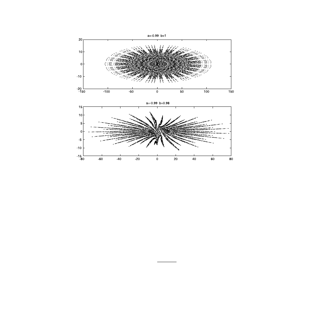
Mira’s Model

The coordinates of the points on the Mira curve are generated iteratively
through the following system of nonlinear difference equations:

(2.43)

where

(2.44)

We illustrate the different morphologies of the solutions in two different
cases, and leave other cases as exercises for your fun and exploration.

FIGURE 2.2
Plot of the Mira curve for a = 0.99. The starting point coordinates are (4, 0). Top panel: b =
1, bottom panel: b = 0.98.

x k

by k

F x k

y k

x k

F x k

(

)

( )

( ( ))

(

)

( )

(( (

)))

+ =

+ = −

F x

a x

( )

(

)

−
+

2 1

Case 1

Here, a = –0.99, and we consider the cases b = 1 and b = 0.98. The

starting point coordinates are (4, 0). See

Figure 2.2

. This case can be viewed

by editing and executing the following script M-file:

for n=1:12000

a=-0.99;b1=1;b2=0.98;

x1(1)=4;y1(1)=0;x2(1)=4;y2(1)=0;

x1(n+1)=b1*y1(n)+a*x1(n)+2*(1-a)*(x1(n))^2/(1+

(x1(n)^2));

y1(n+1)=-x1(n)+a*x1(n+1)+2*(1-a)*(x1(n+1)^2)/(1+

(x1(n+1)^2));

x2(n+1)=b2*y2(n)+a*x2(n)+2*(1-a)*(x2(n))^2/(1+

(x2(n)^2));

y2(n+1)=-x2(n)+a*x2(n+1)+2*(1-a)*(x2(n+1)^2)/(1+

(x2(n+1)^2));

end

subplot(2,1,1); plot(x1,y1,'.')

title('a=-0.99 b=1')

subplot(2,1,2); plot(x2,y2,'.')

title('a=-0.99 b=0.98')

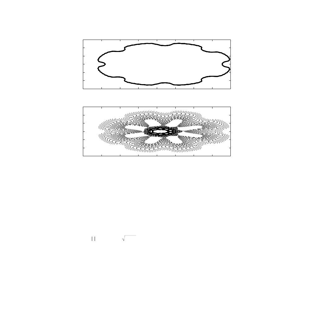
Case 2

Here, a = 0.7, and we consider the cases b = 1 and b = 0.9998. The

starting point coordinates are (0, 12.1). See

Figure 2.3

In-Class Exercise

Pb. 2.23

Manifest the computer artist inside yourself. Generate new geo-

metrical morphologies, in Mira’s model, by new choices of the parameters
(–1 < a < 1 and b

≈ 1) and of the starting point. You can start with:

x y

0 48

0 93

4 0

0 25

0 99

3 0

0 1

0 99

3 0

0 5

0 9998

3 0

0 99

0 9998

0 12

( ,

)

( , )

( ,

)

−
−

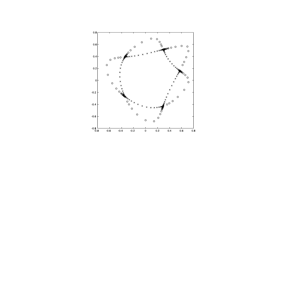
2.8.2

Hénon’s Model

The coordinates of the Hénon’s orbits are generated iteratively through the
following system of nonlinear difference equations:

(2.45)

where

Executing the following script M-file illustrates the possibility of generating

two distinct orbits if the starting points of the iteration are slightly different
(here, a = 0.24), and the starting points are slightly different from each other.
The two cases initial point coordinates are given, respectively, by (0.5696,
0.1622) and (0.5650, 0.1650). See

Figure 2.4

a=0.24;

b=0.9708;

FIGURE 2.3
Plot of the Mira curve for a = 0.7. The starting point coordinates are (0, 12.1). Top panel: b
= 1, bottom panel: b = 0.9998.

-20

-15

-10

-5

-15

-10

-5

a=0.7 b=1

-20

-15

-10

-5

-15

-10

-5

a=0.7 b=0.9998

x k

ax k

b y k

x k

y k

bx k

a y k

x k

(

)

(

)

( ( ) ( ( )) )

(

)

(

)

( ( ) ( ( )) )

+ =

+ −

−

+ =

+ +

−

≤

−

and

x1(1)=0.5696;y1(1)=0.1622;

x2(1)=0.5650;y2(1)=0.1650;

for n=1:120

x1(n+1)=a*x1(n)-b*(y1(n)-(x1(n))^2);

y1(n+1)=b*x1(n)+a*(y1(n)-(x1(n))^2);

x2(n+1)=a*x2(n)-b*(y2(n)-(x2(n))^2);

y2(n+1)=b*x2(n)+a*(y2(n)-(x2(n))^2);

end

plot(x1,y1,'ro',x2,y2,'bx')

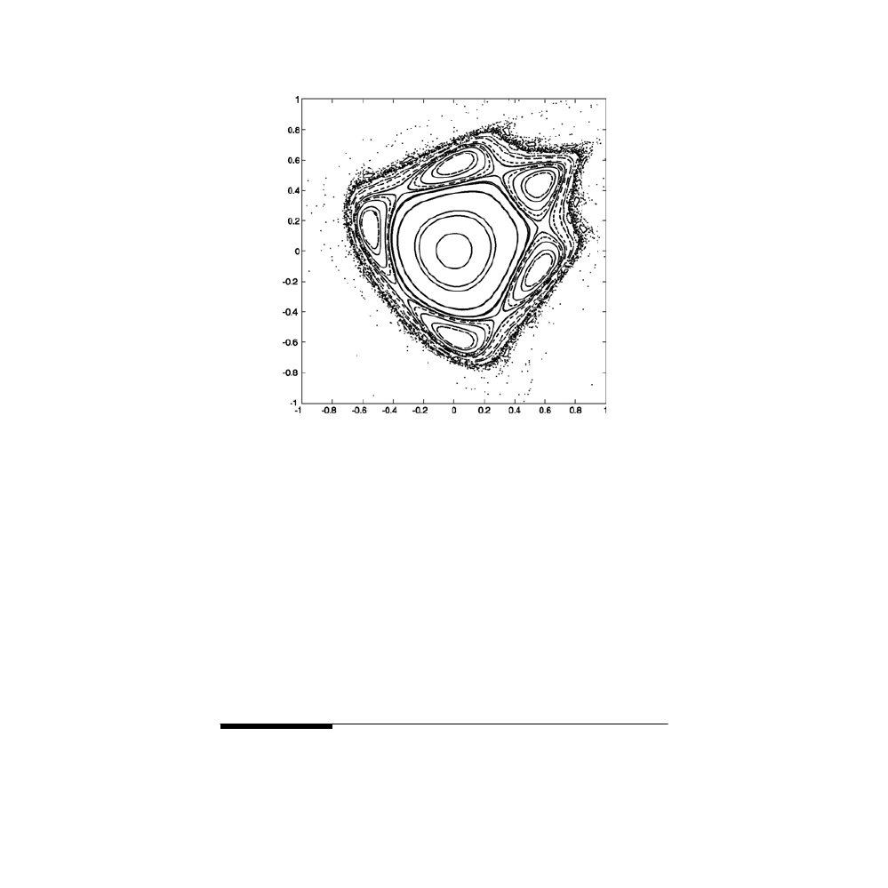
2.8.2.1

Demonstration

Different orbits for Hénon’s model can be plotted if different starting points
are randomly chosen. Executing the following script M-file illustrates the a =
0.24 case, with random initial conditions. See

Figure 2.5

a=0.24;

b=sqrt(1-a^2);

rx=rand(1,40);

ry=rand(1,40);

FIGURE 2.4
Plot of two Hénon orbits having the same a = 0.25 but different starting points. (o) corre-
sponds to the orbit with starting point (0.5696, 0.1622), (x) corresponds to the orbit with
starting point (0.5650, 0.1650).

for n=1:1500

for m=1:40

x(1,m)=-0.99+2*rx(m);

y(1,m)=-0.99+2*ry(m);

x(n+1,m)=a*x(n,m)-b*(y(n,m)-(x(n,m))^2);

y(n+1,m)=b*x(n,m)+a*(y(n,m)-(x(n,m))^2);

end

plot(x,y,'r.')

axis([-1 1 -1 1])

axis square

2.9

Generation of Special Functions from Their Recursion
Relations*

In this section, we go back to more classical mathematics. We consider the
case of the special functions of mathematical physics. In this case, we need to

FIGURE 2.5
Plot of multiple Hénon orbits having the same a = 0.25 but random starting points.

define the iterated quantities by two indices: the order of the function and the
value of the argument of the function.

In many electrical engineering problems, it is convenient to use a class of

polynomials called the orthogonal polynomials. For example, in filter design,
the set of Chebyshev polynomials are of particular interest.

The Chebyshev polynomials can be defined through recursion relations,

which are similar to difference equations and relate the value of a polynomial
of a certain order at a particular point to the values of the polynomials of
lower orders at the same point. These are defined through the following
recursion relation:

(x) = 2xT

k–1

(x) – T

k–2

(x)

(2.46)

Now, instead of giving two values for the initial conditions as we would have
in difference equations, we need to give the explicit functions for two of the
lower-order polynomials. For example, the first- and second-order Cheby-
shev polynomials are

(x) = x

(2.47)

(x) = 2x

– 1

(2.48)

Example 2.7

Plot over the interval 0

≤ x ≤ 1, the fifth-order Chebyshev polynomial.

Solution:

The strategy to solve this problem is to build an array to represent

the x-interval, and then use the difference equation routine to find the value
of the Chebyshev polynomial at each value of the array, remembering that
the indexing should always be a positive integer.

The following program implements the above strategy:

N=5;

x1=1:101;

x=(x1-1)/100;

T(1,x1)=x;

T(2,x1)=2*x.^2-1;

for k=3:N

T(k,x1)=2.*x.*T(k-1,x1)-T(k-2,x1);

end

y=T(N,x1);

plot(x,y)

In-Class Exercise

Pb. 2.24

By comparing their plots, verify that the above definition for the

Chebyshev polynomial gives the same graph as that obtained from the
closed-form expression:

(x) = cos(N cos

–1

(x)) for 0

≤ x ≤ 1

In addition to the Chebyshev polynomials, you will encounter other

orthogonal polynomials in your engineering studies. In particular, the solu-
tions of a number of problems in electromagnetic theory and in quantum
mechanics (QM) call on the Legendre, Hermite, Laguerre polynomials, etc. In
the following exercises, we explore, in a preliminary manner, some of these
polynomials. We also explore another important type of the special functions:
the spherical Bessel function.

Homework Problems

Pb. 2.25

Plot the function y defined, in each case:

Legendre polynomials:

For 0

≤ x ≤ 1, plot y = P

(x)

These polynomials describe the electric field distribution from a nonspherical
charge distribution.

Hermite polynomials:

For

The function y describes the QM wave-function of the harmonic oscillator.

Laguerre polynomials:

For 0

≤ x ≤ 6, plot y = exp(–x/2)L

(x)

The Laguerre polynomials figure in the solutions of the QM problem of
atoms and molecules.

(

)

( ) (

)

( ) (

)

( )

(

)

P x

−

1
2

and

H x

−







( )

(

)

( )

and

1 2

≤ ≤

−

A H x

( ) exp(

/ ),

(

)

plot

where

x L

L x

x x

+ −

−

= −







3 2

1 2

( ) [(

)

( ) (

)

( )]/ (

)

( )

( ) (

/ )

and

Pb. 2.26

The recursion relations can, in addition to defining orthogonal

polynomials, also define some special functions of mathematical physics. For
example, the spherical Bessel functions that play an important role in defin-
ing the modes of spherical cavities in electrodynamics and scattering ampli-
tudes in both classical and quantum physics are defined through the
following recursion relation:

With

Plot j

(x) over the interval 0 < x < 15.

j x









−







−

3 2

( )

sin( )

cos( )

( )

sin( )

cos( )

and

Document Outline

ELEMENTARY MATHEMATICAL and COMPUTATIONAL TOOLS for ELECTRICAL and COMPUTER ENGINEERS USING MATLAB ®
- Table of Contents
- Chapter Two
  - Difference Equations

Wyszukiwarka

Podobne podstrony:
1080 PDF C09
1080 PDF C07
1080 PDF C08
1080 PDF C10
1080 PDF ADDE
1080 PDF C04
1080 PDF C06
1080 PDF C03
1080 PDF TOC
1080 PDF C01
1080 PDF C05
1080 PDF REF
1080 PDF C09
1080 PDF C07
1080 PDF C08
instr 2011 pdf, Roztw Spektrofoto
(ebook PDF)Shannon A Mathematical Theory Of Communication RXK2WIS2ZEJTDZ75G7VI3OC6ZO2P57GO3E27QNQ
KSIĄŻKA OBIEKTU pdf
zsf w3 pdf

więcej podobnych podstron

1080 PDF C02

Document Outline