Olsztyn, 27th May, 2013

University of Warmia and Mazury in Olsztyn
Faculty of Geodesy and Land Management
Department of Satellite Geodesy and Navigation

ESSAY

Kepler’s equation solution: different methods.

Daria Bruniecka

Geodesy and Satellite Navigation

1st year M.Sc. studies

Kepler’s equation solution: different methods

(M, e) E-esinE=M E=?

In 1609 Kepler published his work Astronomia Nova, containing the first (and the second) law of
planetary motion:

Planets move in elliptical orbits with the sun at one focus.

Between 1617 and 1621 Kepler wrote Epitome Astronomiae Copernicanae, the first astronomy
textbook based on the Copernican model. Kepler introduced what is now known as Kepler's equation
for the solution of planetary orbits, using the eccentric anomaly E, and the mean anomaly M.

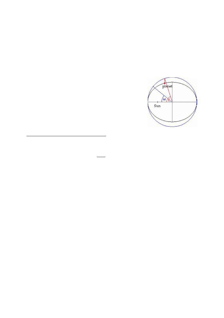
The term anomaly (instead of angle), which means irregularity, is used
by astronomers describing planetary positions. The term originates
from the fact that the observed locations of a planet often showed
small deviations from the predicted data.

The mean anomaly M is the angular distance from perihelion which a
(fictitious) planet would have if it moved on the circle of radius a with
a constant angular velocity and with the same orbital period T as the
real planet moving on the ellipse. By definition, M increases linearly
(uniformly) with time.

Operating with radians the Kepler’s equation is:

( ) −

( ) =

( )

or, using degrees:

( ) −

180°

sin

( ) = ( )

Where:

 M is the mean anomaly (anomalia średnia),
 E is the eccentric anomaly (anomalia mimośrodowa),
 e is the eccentricity (mimośród orbity).

Kepler's equation gives the relation between the polar coordinates of a celestial body (such as a planet)
and the time elapsed from a given initial point. Kepler's equation is of fundamental importance in
celestial mechanics, but cannot be directly inverted in terms of simple functions in order to determine
where the planet will be at a given time.

The value of M at a given time is easily found when the eccentricity e and the eccentric anomaly E are
known. The problem is to find E (from which the position of the planet can be computed) when M and
e are known. Kepler's equation is a transcendental equation because sine is a transcendental function,
meaning it cannot be solved for E algebraically. It can be treated by iteration methods. Numerical
analysis and series expansions are generally required to evaluate E.

Methods of solving the Kepler's equation

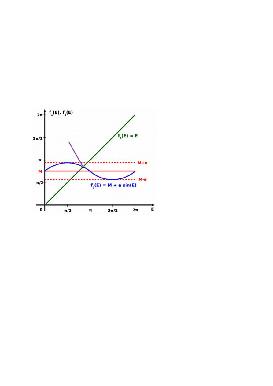
First, this equation can be solved graphically and interpreted as the search for the point of intersection
of the graphs of two functions of the eccentric anomaly.
Kepler’s equation rewrited as follows:

E = M + e sin (E)

So:

f

1

(E) = E,

f

2

(E) = M + e sin(E)

This point is illustrated in below figure:

For obvious reasons, limit is square of
2π × 2π.

On the horizontal axis there is
eccentric anomaly E a and on the
vertical axis there are plots of two
functions f

1

=(E) and f

2

= E (E) = M +

e sin (E).

It is clear that equation always has a
solution, and only one.

It is also visible that the solution is
always in the range
<M-e; M+e>.

The next step in solving the Kepler’s equation is to find a zero approximate solution.

Zero approximation can be calculated in many different ways.

1. If we have some of the values of E for the next few dates get through extrapolation.
2. One of many graphical methods can be used, for example:

 two curves are drawn in one coordinate system (the same diagram):

 and E as a point of intersection is found.

3. If M and e is known development in a number (rozwinięcie w szereg) can be used:

Solution





M

E

e

y

E

y







1

;

sin

M

e

M

e

M

E

2

sin

2

1

sin

2

0







Found zero approximation E

0

may be clarified as follows:

We have:

Where E is exact value. Now ΔE

0

is needed. From Kepler’s equation:

Because ΔE

0

is very small so:

Next procedure is simple iteration since the assumed accuracy is obtained.

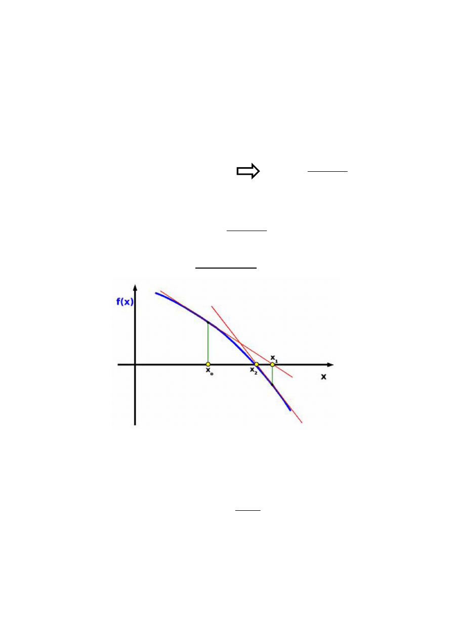
Newton Iteration

The geometric interpretation of Newton's method

This method is based on Kepler’s equation rewritten as:

that gives:

and

f’(E) = −1 + e cosE

0

0

0

0

0

0

0

;

;

sin

E

E

E

M

M

M

E

e

E

M





















0

0

0

0

0

0

sin

E

E

e

E

E

M

M

















0

0

0

0

cos E

E

e

E

M











0

0

0

cos

1

E

e

M

E









k

k

k

k

E

e

M

E

E

cos

1

1











 

0

sin









E

E

e

M

E

F

 

 

n

n

n

n

E

f

E

f

E

E

'

1







Algorithm for Newton's method:

 Choose E

1

= M.

 Update:

=

−

−

+

− 1

 If | E

n+1

- E

n

| < ε where ε is sufficiently small value we can stop calculation.

 Otherwise repeat.

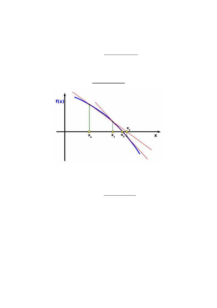
The secant method

The geometric interpretation of secant method

It is a variant of the Newton's method in which the derivative is replaced by the differential quotient.
The formula for further approximation has the form:

=

−

( (

)(

−

))

( (

) − (

))

It can be seen that the method needs to start two initial values E

0

and E

1

, which we calculate E

3

, etc.

As in previous case if | E

n+1

- E

n

| < ε where ε is sufficiently small value we can stop calculation.

There are other useful methods to solve Kepler’s equation, for example:

 Bisection method,

 The method "regula falsi",

 Converting between True and Eccentric Anomaly.