1

Linear viscoelastic model for elongational

viscosity by control theory

Tommi Borg

1

TomCoat Oy, Koskisenkuja 11, 62500 Evijärvi, Finland

Esko J. Pääkkönen

Tampere University of Technology, Laboratory of Plastics and Elastomer
Technology, P.O. Box 589, 33101 Tampere, Finland

Flows involving different types of chain branches have been modelled as functions of the uniaxial

elongation using the recently generated constitutive model and molecular dynamics for linear

viscoelasticity of polymers. Previously control theory was applied to model the relationship

between the relaxation modulus, dynamic and shear viscosity, transient flow effects, power law

and Cox-Merz rule related to the molecular weight distribution (MWD) by melt calibration.

Temperature dependences and dimensions of statistical chain tubes were also modelled. The

present study investigated the elongational viscosity.

We introduced earlier the rheologically effective distribution (RED), which relates very accurately

and linearly to the viscoelastic properties. The newly introduced effective strain hardening

distribution (RED

H

) is related to long-chain branching. This RED

H

is converted to real long-chain

branching distribution (LCBD) by melt calibration and a simple relation formula. The presented

procedure is very effective at characterizing long-chain branches, and also provides information on

their structure and distribution. Accurate simulations of the elongational viscosities of low-density

polyethylene, linear low-density polyethylene and polypropylene, and new types of MWDs are

presented. Models are presented for strain hardening that includes the monotonic increase and

overshoot effects. Since the correct behaviour at large Hencky strains is still unclear, these

theoretical models may aid further research and measurements.

Keywords: Elongational viscosity; Polydispersity; Control theory; Melt

calibration; Long-chain branching

1. Introduction

This paper forms part of a series of papers on the use of control theory to

model the viscoelastic properties of polymers. We first present a formula for

1

To whom correspondence should be addressed.

2

uniaxial elongational viscosity without strain hardening, which is derived in a

similar way to that used in previous studies, by starting from control theory. The

next step involves including the effective strain-hardening distribution, which in

many cases is related to long-chain branching. Some accurate simulation results

related to elongation or extension are also presented.

It is beyond the scope of this article to provide a complete summary of all

the group studies of elongational viscosity; more information on this is available

in the historical reviews by Petrie

1

(for the last 100 years) and Mackley

2

(for the

last 40 years). In recent decades measurements have made by Meissner and

Hostettler,

3

Laun and Schuch,

4

Münstedt

5

, Münstedt et. al.

6, 7

Sentmanat,

8

Hassager et al.

9

, Aho et al.

10

and van Ruymbeke et. al..

11

Fewer studies have modelled the elongational viscosity, among them being

Wagner,

12, 13

Rolón-Garrido and Wagner,

14

Rolón-Garrido et. al.

15

with a

generalization of the theory of Doi and Edwards,

16 , 17

Laun

18

on memory function,

Rauschenberger and Laun

19

on recursive model, McLeish and Larson

20

and

Inkson et al.

21

on “pom-pom” constitutive equations, Likhtman and Graham

22

on

the Roli-poly model, Auhl et. al.

23

on the volume of tube and van Ruymbeke et.

al.

24

by Mixing law and tube pressure.

We have previously published separate studies for different types of

viscoelastic flows as relaxation modulus,

25

dynamic

26

and shear viscosity

27

related

to the rheologically effective distribution (RED) and further molecular weight

distribution (MWD). Temperature dependences and dimensions of statistical

chain tubes were also modelled.

28

These papers explain more background for the

used control theory, chain dynamics and developments of formulas.

Among other this study explains why dynamic frequency sweep

measurements with oscillation rheometer with presence of possible amount of

LCBs are preferred to carry out at constant strain controlled mode instead of

widely used stress controlled mode.

The short review of the principle

General principle of control theory and models for elementary

viscoelasticity are reviewed shortly. The modern control theory is used in many

modern technologies as digital computers, aircrafts and process industry. As

3

control theory itself is mathematically well accepted principle over hundred years,

procedure creates also to the target formulas linear model.

We excite the system with a small stress induced by a small pulsed strain

that is applied at time t

0

. Pulse response y(t) is obtained from impulse response

h(t) and by sampling the active molecules in distribution w(t) between some time

interval:

d

(1)

This equation is a familiar linear formula used in control theory, which is

known as a novel principle to adjust and rule by one variable or function in a

closed system and now in our case for rheologically effective distribution (RED)

or w(t) related to the MWD. This convolution integral differs from respective

Maxwell type and Mixing laws as the functional Eq. (1) has no relaxation time

procedures or variables at different scales. Thus there are fundamental differences

in relaxation times λ and their discrete spectra are artificial, whereas continuous

distribution RED w(t) is a true function in the form of statistical distribution for

viscoelastic effects and later related to the MWD.

Pulse response

log

log

is a normalized relaxation modulus with

a maximum value of zero on the logarithmic scale at t

0

. The value for zero

relaxation modulus G

0

= G(t

0

) is obtained by fitting G(t) to experimental

measurements. We then obtain the complete relaxation formula in the case where

a small and constant strain is induced:

, (2)

where impulse response

log

log

log and value for elastic constant

P is obtained by feedback procedure of control theory. Presented Eq. (2) models

accurately relaxation phenomena although viscous component and constant P" is

not yet included as is discussed in more detailed explanation for relaxation

modulus in Part I.

25

Originally, we applied formula for modelling viscoelastic flows to get out

computed MWD as we did in Part II.

26

The power of control theory is the fact

that it reduces the need for using variables as we did in the Parts I–IV.

25–28

During studies this same power was used to develop at first accurate

viscoelastic fits for different flows and after that were found relations to the other

microstructures as statistical tube dimensions discussed in Part IV. Thus our

4

development processes were done on the contrary as by earlier studies.

12–24

This

unusual procedure guarantees accurate, simple but consistency model with

physics for these complicated phenomena and flows. In other words we can go by

step by step downwards for more detailed and complicated microstructures and

still keeping the consistency of the model. The strength is the fact that polymer

chain structure complexity is not limitation for good semi-empirical viscosity

models and more challenge is coming from studying chain microstructure.

Already is published over sixty different new equations for different flows

without using artificial relaxation time schema. As principle starts on a clean

table and on new standpoint in rheology, developments cannot be evaluated by

such as Occam's razor principle. Actually only few material dependent constants

are used.

Until very recently was found that rheologically effective distribution

(RED), which relates very accurately and linearly to the viscoelastic properties, is

actually melt chromatogram as in liquid chromatography methods eluent, elution

curve or elugram.

Model Development

Elongational viscosity

without strain hardening effect

We can directly write the formula in the start-up for uniaxial elongational

viscosity

E

using control theory in a similar way to previous work on the

relaxation modulus and the dynamic and shear viscosities. The strain hardening

effects coming from long-chain branches (LCBs) or similar structures are not yet

included in to the elongational viscosity

. As previously for the case in the

start-up of shear viscosity being a function of shear and elongation, we have to

use our new time–rate separability basis (which is new to rheology) when deriving

functions for the parallel-resistor analogy

27

. Now the elongation is again a

function of one rate variable, , and hence we do not need to start from steady-

state elongational viscosity

η

—which is a function of constant Hencky

strain rate

and constant tensile stress . Moreover, the steady-state

elongational viscosity or “Trouton viscosity” is difficult to measure.

5

We use an alternative strategy to get elongational viscosity by imposing

net tensile stress

E

monitoring as a function of time. At first we model

E

without any strain-hardening effects or influences of LCBs.

Thus, we write a characteristic formula directly for elongational viscosity

E

, where the tilde mark over the “ ” indicates that the strain-hardening effect

is not yet included:

log

E

log

log

log

(3)

where

is the elongational viscosity at characteristic time t

c

= 1/s similar way as

earlier. We developed the formula similar way starting from control theory as for

characteristic relaxation modulus G

c

(t) by Eq. (13),

25

characteristic complex

viscosity by Eq. (7)

26

and characteristic shear viscosity by Eq. (1).

27

The

rheologically effective distribution (RED) w(log t) relates not only to orientated

but also stretched chains that lose their entanglements. RED function w(t) can be

regarded as respective chromatogram or elugram distribution with liquid

chromatography of GPC/SEC. This RED, presenting here as an elastic

component, influences the polymer normally after t > 0.001 s during elongation.

Since the possible measurement range starts after t > 0.01 s, we do not need to use

the w''(log t) component of the RED'' distribution including viscoelastic effects,

since it is always at normalized value w'' = 1 in these measurement ranges and

hence can be simplified to P''w''(log t) = P''. In most cases P > 0, but always P'' <

0.

A simple relation can be written for the melt calibration, M(t), as a

function of time, where the value of Mf is M at

1/ :

(4)

This formula can be used to convert MWD w(log M) into RED w(log t) or

w(log t) = w(log M). Melt calibration has close similarities with the widely used

linear broad-standard calibration with SEC, which approach requires a broad

standard of known number-average M

n

and weight-average M

w

molecular

weights. The use of different Mf and Hf values allows the REDs to be converted

into their respectively MWDs, where Mf sets the absolute molecular weight and

Hf sets the polydispersity value.

6

The analytical formula for viscosity

η

E

t can be written by applying a

procedure similar to that used in our previous studies, but this was not required for

the present study.

Strain hardening with a monotonically increasing effect

Elongational viscosity

E

includes basic strain-hardening component

originally

H

log ) as a function of time t and elongation rate or effective

strain-hardening distribution

H

log , ), where

with monotonically

increasing behaviour, at least in the absence of the overshoot effect, as has been

done in most other simulation models.

Long-chain branches (LCBs) and high-molecular-weight (HMW) end

fractions impact strain-hardening effects on the initial elongation in elongation

experiments. The origin of this additional response is the oriented and taut tied

stretched chains between entanglements that did not have time to disentangle and

relax. The longest chains are the first to exhibit this taut tied characteristic, and

strong strain hardening begins to occur since they have no more free loops

anywhere. Finally the flow becomes non-homogeneous on a micro or even a

semi-micro scale, which accelerates the breakdown of elongation experiments.

Since hardening is related to the length of chains, LCBs and HMW end

fractions, we set the respective hardening and rheologically effective distribution

RED

H

or

H

, ) (note that we are using the “H” subscript, even though the

origin can also be other than LCBs or HMW end fractions). The strain-hardening

effect is adjusted by the value of P

H

. Now we can write the complete formula for

start-up of elongational viscosity

as

log

,

log

log

log ,

log (5)

For developing RED

log ,

H

we use its own RED

H

according to Eq.

(4) with its own Mf and Hf factors, since this rheological behaviour is totally

different.

From the standpoint of molecular dynamics and the tube model described

previously,

28

we obtain that statistical unit segment length L

s

increases and

diameter D

s

decrease relatively for a unit backbone during elongation. Elasticity

function

′

′

and especially

H

decrease in a similar way in Eq. (5) giving

less strain hardening effect.

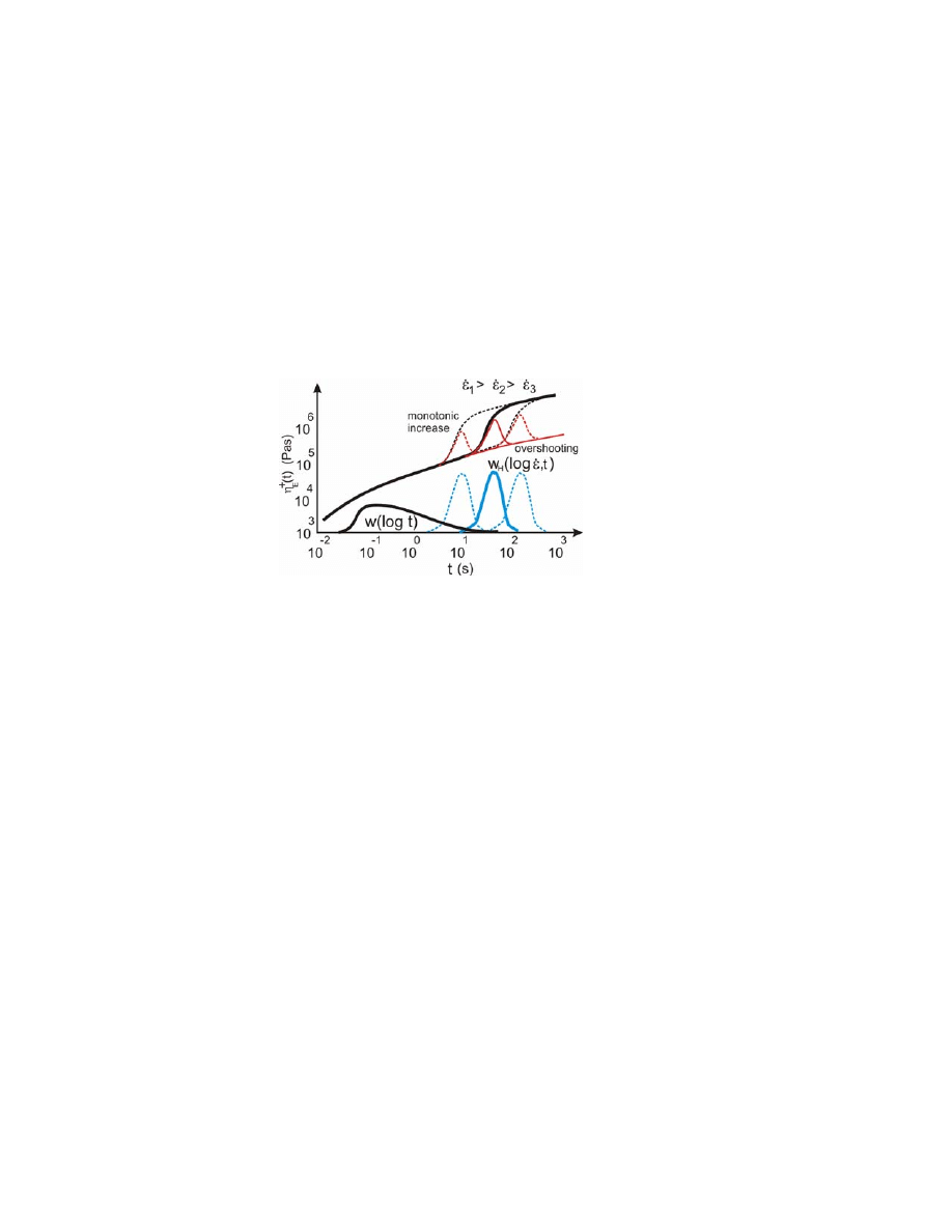
7

For the used elongation rates, with <1/s, meaningful differences to

values are not observed at the beginning (i.e., t < 0.1 s), but the amount of strain

hardening depends on the used rate described by strain-hardening coefficient χ(t,

).

29,

30

They discuss the molecular structure, referring to long-chain branching.

But no simulation model is presented for absolute measured values of χ(t, ), thus

we have to develop a simple model to perform modelling and obtain simulation

results. The strain-hardening effect, P

H

( ), is linearly related to strain-hardening

coefficient χ(t, ). Normalized distributions w(log t) and w(t, ) and strain

hardening effects during different strain rates are shown in Fig. 1.

Figure 1. Elongational viscosity

η

E

t with LCBs giving strain hardening, and a schematic model

for converting REDs and REDHs into the respective MWDs. RED

H

s are scaled with their

effectiveness by

P

H

(

ε) values or P

H

ε w

H

log t, ε), where ε

εt at different elongation rates

according to Eq. (5) for a monotonic increase and Eq. (6) for the overshoot strain-hardening

effects.

The above-described procedure for simulations is rather insensitive to the

actual form of the used MWD, which make it possible to use MWD data copied

from the literature or to use nominal distributions. The results are much more

sensitive to the actual form of the LCBD and

H

, ).

Strain-hardening component

, ) with the overshoot property

The elongational viscosity at large strains has been studied less, as has

strain-hardening viscosity. Rasmussen et al.

31

measured the viscosity at large

Hencky strains of up to 6–7 for low-density polyethylene (LDPE) as shown in

Fig. 3 and linear low-density polyethylene (LLDPE). They observed that LLDPE

behaves as shown in Fig. 4 and according to Eq. (5), whereas LDPE exhibits a

viscosity overshoot effect that appears as a bump. We thus rewrite Eq. (5) for the

overshoot-type strain hardening as follows:

8

log

log

log

log

log ,

(6)

The form of the left side of strain-hardening distribution

log , is

similar to that at the beginning of strain hardening from Eq. (5) or (6). However,

the final form of the subsequent strain hardening remains unclear.

Burghelea et al.

32

very recently argued that the overshoot phenomena are

not real rheological features but rather merely represent artefacts resulting from

the strong geometric non-uniformity of the sample at high Hencky strains. If it

does exist, strain hardening could be described as a mixture of Eqs. (5) and (6),

but we are unable to derive these combined formulas since there are insufficient

data available at high Hencky strains. Fortunately this has little effect on the

obtained left side of strain-hardening distribution RED

H

or the right side of

LCBD.

Effective strain-hardening distribution RED

H

from elongational

viscosity measurements

We extract strain-hardening distribution RED

H

from Eq. (5) using a

procedure similar to that described for the relaxation modulus

25

or shear

viscosity

26

. We obtain

H

log , ) by deriving as follows from the measured

differences to

to accurately obtain the shape of the RED

H

curve:

log ,

log

log (7)

Eq. (6) or a mixture of Eqs. (5) and (6) can be solved in a similar way to

obtain RED

H

, but this was not done in this study.

Long-chain branching distribution

Strain-hardening distribution RED

H

is converted to direct relation of long-

chain branching distribution (LCBD) by melt calibration with a simple relation

formula. Real distributions for LCBDs have very rarely presented with MWD in

literature.

9

A nuclear magnetic resonance method (NMR) is used to detect LCB, but

is known that NMR can be used to detect side chain branches with up to 8 carbon

atoms only.

33

Many alternative ways have been developed to obtain a single

numerical value

34, 35, 36, 37, 38, 39

including by utilizing the Zimm–Stockmayer

equation.

40

Several rheological methods are suitable for identifying LCB,

41, 42, 43,

44, 45, 46

such as van Gurp–Palmen

47, 48

and Cole–Cole

49

plots, flow activation

energy,

50

thermorheology,

51

the dynamic modulus,

41

and relaxation times,

but all

suffer from the problem of not being able to convert the obtained results into

absolute numerical values.

Applying a stochastic approach to topological LCBD models has yielded

the multidimensional distributed molecular properties (e.g., joint MW–LCB

distribution) with the number of long chain branches.

52, 53, 54

We employ a different procedure using a more realistic one-dimensional

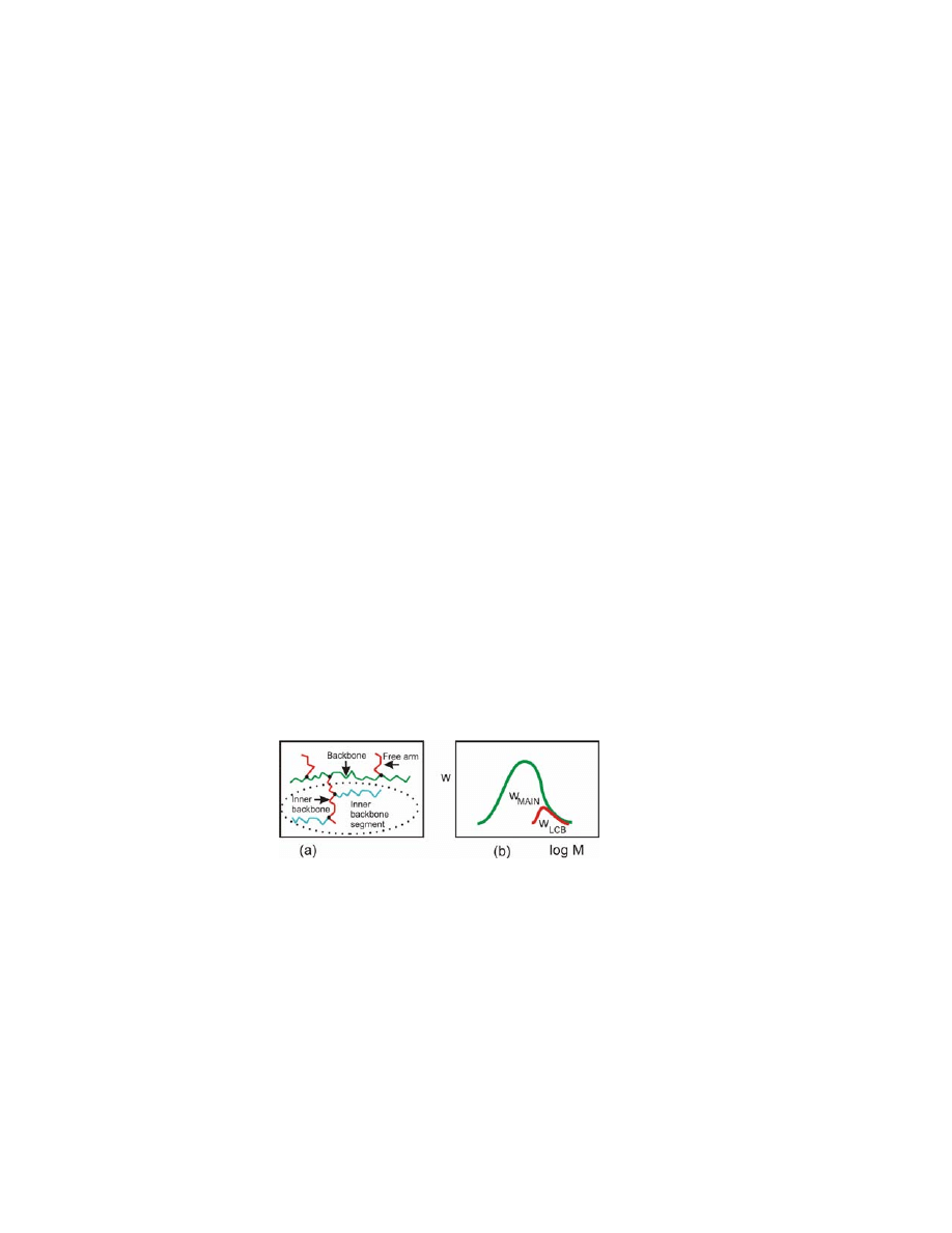
LCBD with the total number of inner backbones. In Fig. 2a on the left is shown

used terminology

55

for the primary chain as backbone, directly linked chains are

free arms and next connected chains are inner backbone segments. Of course this

LCBD in Fig 2b can be fractionalized later on to bivariate MW–LCB distribution

if needed.

54

Main distribution w

MAIN

(M) can be detected rheologically

26

or by

GPC/SEC, which is used mainly for this study and known also insensitive to

detect LCBs. For showing final results we use sum of RED or MWD

distributions to get normalized sum value one as follows: ∫w

MAIN

+∫w

LCB

= 1.

Figure 2. Schematic diagram of detecting LCBD w

LCB

(M).

a. Molecule chain has backbone, free arms and inner backbone segments.

b. From GPC/SEC or by using narrow dynamic viscoelastic data range to get normalized MWD

or w

MAIN

(M). From strain-hardening distribution

log , and own Mf and Hf values for melt

calibration we get absolute LCBD or w

LCB

(M) distribution.

LCB distribution as a function of M or

log , , where

1/s used in this study, is gained by the right selection for Eq. (4) by their own

values Mf and Hf for melt calibration similar way as are done with calibration

curve and GPC/SEC procedures. As constants P and P

H

set effects for

10

viscoelastic properties and they are inside log function, we get simple formula for

strain-hardening coefficient χ( ) = log (P

H

( /P) as both constants in Eq. (5) are

inside logarithm. The influence of right size for final LCB distribution w

LCB

(M)

by using relation 1/χ of normalized MWD and LCBD as follows

log

,

(8)

where M

b

is molar mass m of a backbone element, for PE M

b

= 14mol/g.

In principle LCBD can be outside of MWD even though measured by GPC/SEC,

as these methods do not detect LCBs. Thus we get absolute LCBD or w

LCB

(M) by

using different structural value Mf and conversion factor Hf for conversion from

RED

H

.

We can renew the formula for the LCB frequency—expressed as the

number of long chain branches per 1,000 carbon atoms as presented in previous

studies

39, 45

—using the above results for LCBD as follows:

LCB

1000 C

1000

∑

LCB

(9)

where w

LCB

is the weight fraction of LCBD, M

i

is the MW of each

fraction, and M

b

is the molar mass of a backbone element [M

b

= 14 for

polyethylene (PE)]. Complete weight fraction w

i

of the MWD and the average

number of branches per molecule were originally used in the formula.

39

However,

now this value consists not only of branches on the backbone but also of inner

backbones, as shown in Fig 2a. A major disadvantage of these types of formulas is

that the average MW of backbones (and now branches) strongly influence the

obtained values.

Experimental Section

Test polymers and constants

Strain hardening that occurs during elongation of a branched structure was

modelled. The measured elongational viscosity was simulated as a function of

different elongation rates using control theory, including for higher Hencky

strains that have not yet been measured. The results are compared here with those

that have been observed, and we also discuss more generally used principles,

11

hypotheses, and structures of models and formulas. The measurements made by

Stadler et al.

30

and Münstedt et al.

56

were simulated.

The MWD was measured carried by a high-temperature GPC coupled with

a multiangle light-scattering apparatus (MALLS). MWD for LDPE come from

RheoPower Database. As we know, GPC is not sensitive to detect LCBs.

Elongational viscosity simulations were performed by executing a

characteristic model of control theory on a standard PC with the commercial

RheoPower software package using the RheoDeveloper program with

experimental elongation moduli. We did not need to use the more sensitive

RheoAnalyzer program for MWDs, since their effects on the rheological

properties are less than those of LCBDs in this application. Our description of

results starts by using functional formulas of Eq. (3) giving accurate real fits with

measurements by adjusting RED

H

, then is shown and discussed different

strategies for modelling elongational viscosity at high Hencky strains. Along

calculation is some words of LCB average chain length and distribution and

branching intensity. One bivariate RED- RED

H

distribution chart as a function of

time and rate is shown and finally MW-LCB distribution results converted to two

apparent MWD charts.

Procedure

The elongational viscosity was modelled first without and then with strain

hardening. Since the presented formulas are new, and hence the values of

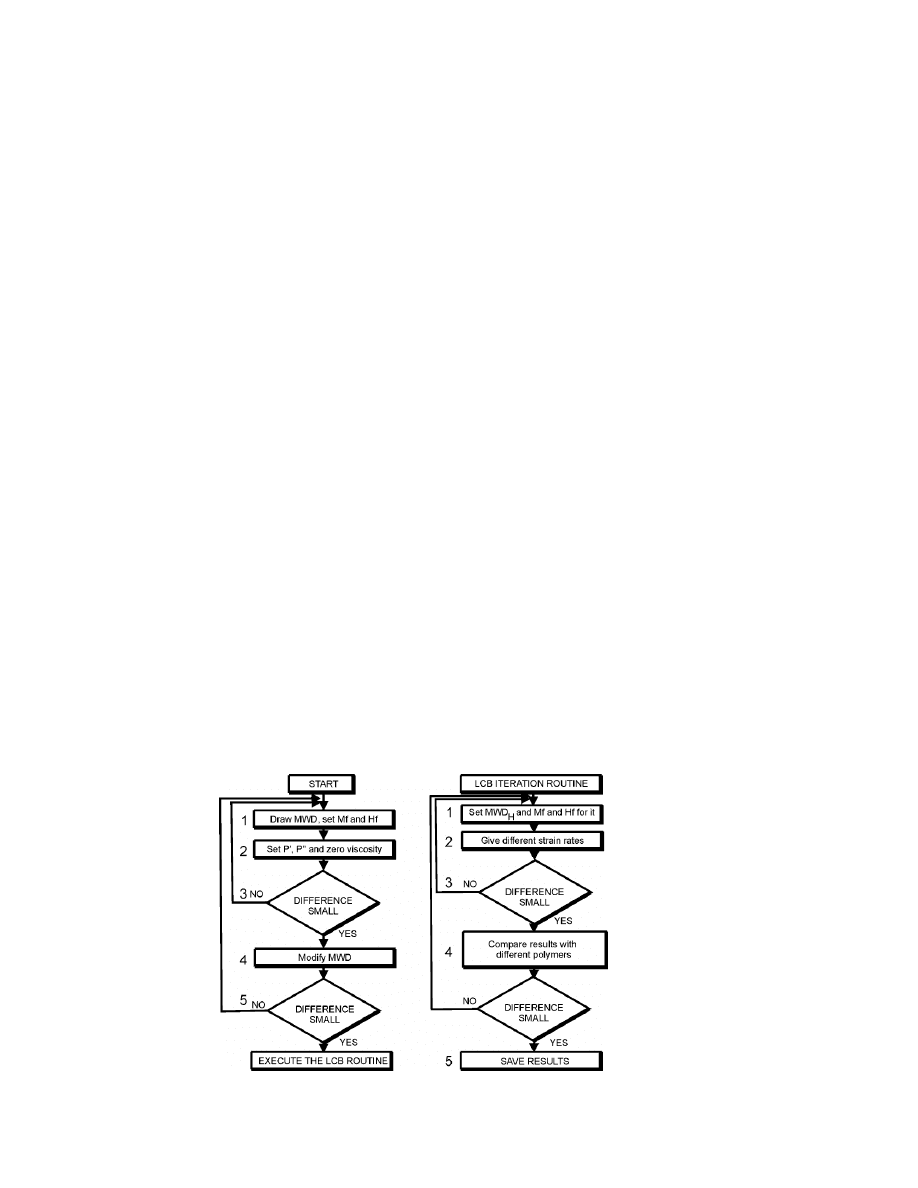
constants are unknown, we explain the step-by-step best-fit routine and by Fig. 3

based on the measurements and our model starting from control theory. We did

not use Eq. (7) to detect

H

log , ) in this study, since we fitted our curves with

previously published measured data. We obtained that manually copied data to

derive by Eq. (7) was sensitive to errors. The elongational viscosity is first

developed without the strain-hardening effect, which involves the following steps:

1. Draw a known MWD in the RheoDeveloper program and save it in

a database. Set Mf and Hf constants as a-priori information using

values found previously for the complex viscosity.

2. Set first test P', P'' and zero

values for the polymer sample, and

compute and compare them with measured elongation values.

12

Adjust the values so that the simulation result on the output chart is

as close as possible to images imported from measured data.

3. Alter the Mf and Hf values and repeat step 2.

4. Modify and alter a little-known MWD to see if errors between the

modeled and measured results increase so as to check if the used

MWD is acceptable.

5. Test different types of polymer samples in order to ascertain the

correct values for constants. Repeat the above steps as many times

as necessary to obtain satisfactory results, at which point you can

proceed to the next level.

The following LCBD iteration routine involves the strain-hardening

function and distribution:

1. Set separate Mf and MwR values for hardening distribution RED

H

H

log , ) with strain-hardening constant P

H

> 0.

2. Obtain some elongation rates and compare them with

measurements. If necessary, select new Mf and Hf constants for

H

log , ).

3. Check the values with different polymers and attempt the obtain the

best fit by using different Mf, Hf,

E

, P

H

( ) and values.

4. You can try to get better fit by drawing manually hardening

distribution RED

H

log , ).

5. Save the final results in ASCII format in log-0.2 steps on a wide

timescale and on the strain rate matrix.

Figure 3. Flowchart of the simulation procedure.

13

The data can be processed further on a spreadsheet such as Excel

®

so as to

combine MWD and LCBD. Measured data can be joined in CAD such as using

the CorelDraw

®

program with the modelled and simulated results.

Results and Discussion

Used main characteristics

A polymer structure is modelled by the values P', P'' and zero viscosity ,

polymer structural value Mf and conversion factor Hf between scales. The values

of P' and P'' obtained from the viscosity fitting procedure are listed in Table 1, and

no ad hoc constants or values were used. A constant temperature of T = 150°C

was used for LDPE and LLDPE, while T = 180°C was used for polypropylene

(PP).

For the effective strain-hardening distribution LCBD we used constant

value Hf = 0.6 to allow comparisons between different samples. The used Mf

values might not be accurate, but it is within the correct range and of course its

value differs at least for PP.

The main characteristics of the samples are listed in Table 1.

LDPE

LLDPE

PP

2

CSTR-LDPE

1

CSTR-LDPE 2

Mw

a

213,000

102,000

574,000

4,167,000 2,271,000

MwR

a

12.9 3.2 9.3 21.4

14.3

Mf

b

70,000

30,000

200,000

70,000 70,000

Hf

b

2.05

2.05 4 2.05 2.05

c

4.6 4.68 4.1 4.87

4.18

P'

d

0.42

0.65

0.56 0.22 0.51

P''

d

–0.7

–0.7

–0.8 –0.68 –0.68

P

H

e

2.6 2 2.6 4

3.4

Mw LCBD

f

10,640,000 9,670,000 7,150,000 17,030,000

9,670,000

MwR LCBD

f

5.3

2.7

1.4

6.5

2.7

Mf

g

4,000,000 4,000,000 4,000,000

40,000,000

40,000,000

Χ

1.8 1.1 1.5 2.9

1.9

LCB/1000

C

h

0.022 0.012 0.034 0.001

0.002

Table 1. Main characteristics of all investigated samples and computations.

a

The used Mw (g/mol) and MwR values may differ slightly from those measured using GPC/SEC.

b

Polymer structural value Mf (g/mol) and conversion factor between scale Hf.

c

Elongational viscosity (Pas) at t = 1/s.

d

Obtained elasticity P' and P'' viscosity values.

14

e

Strain-hardening constant P

H

at rate =1/s.

f

Mw (g/mol) and MwR values obtained for the effective strain-hardening distribution.

g

Polymer structural value Mf (g/mol) for strain-hardening distribution, Hf = 0.6.

h

Strain-hardening coefficient χ( ) at rate =1/s.

i

Long chain branching frequency per 1000

C carbon atoms.

Uniaxial elongational viscosity as a function P

H

( )

We model uniaxial elongational viscosity according to measurements, but

at a much higher Hencky strain (ε) compared to that obtained in practical

measurements (this topic is discussed in Section 4). We first simulate a modern

LDPE (Lupolen 1840 H) for well known and classical IUPAC A, as done

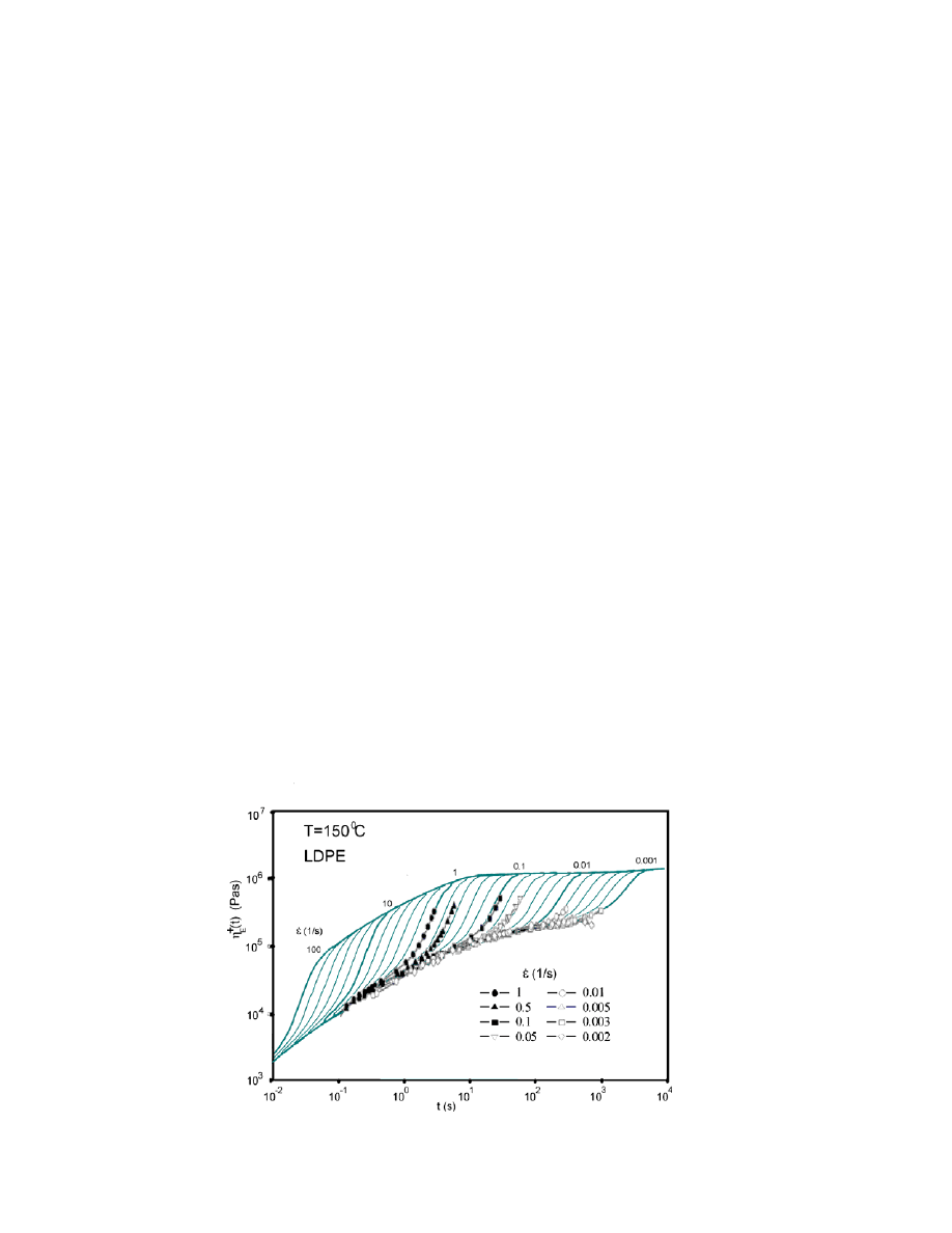
previously our studies. The elongation viscosity results are shown in Fig. 4 and

used RED

H

functionals with P

H

( ) in Fig. 5 according to Eq. (5).

We observe that simulation results accurately fit the measurements made

by Münstedt et al..

56

Since the elongation software moduli of the RheoDeveloper

program was still an experimental version, the output of the elongation viscosity

was still in log-0.2 steps, which corresponds to the following elongation rates:

0.01/s, 0.016/s, 0.025/s, 0.04/s, 0.06/s, 0.1/s, 0.16/s, 0.25/s, 0.40/s, 0.6/s and 1/s.

On the other hand, elongation rates of 0.01/s, 0.1/s and 1/s were used during

measurements, whereas the data were for 0.002/s, 0.003/s, 0.03/s, 0.05/s and 0.5/s,

which fall between the modelled elongation rates.

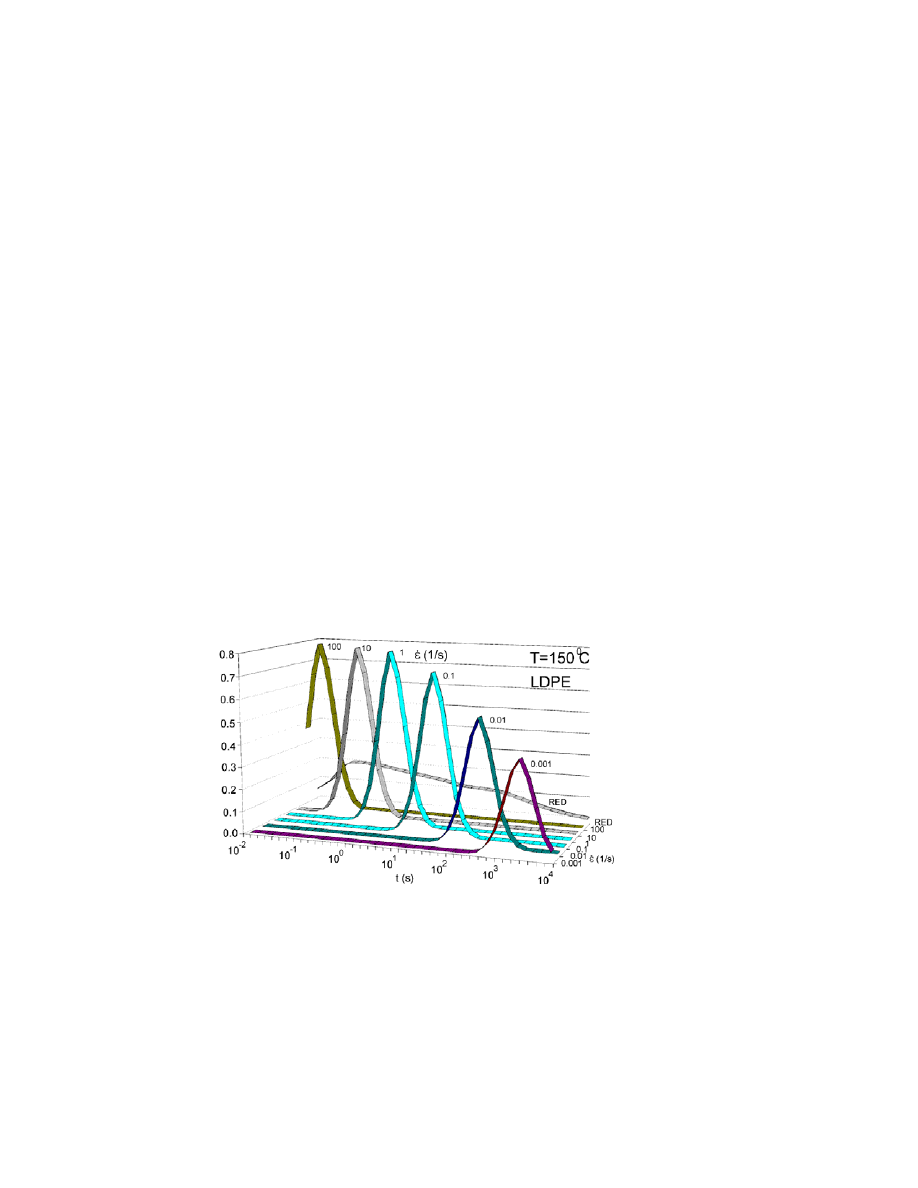
15

Figure 4. Modelled steady elongational viscosity

flow curves as functions of time for

different elongation rates ( ) from 0.001 to 100 s (lines), and data measured by Münstedt et al. for

LDPE (symbols).

56

Modelled rates on decades (e.g., 10/s, 1/s and 0.1/s) are indicated by thicker

lines.

As steady-state elongation viscosity is sometimes thought to run through a

maximum as a function of elongation rate, we can simulate this by using smaller

strain-hardening constants P

H

at higher elongation rates. Used products for Fig. 4

this time variable P

H

( ) as a function of rate and effective strain-hardening

distribution RED

H

or P

H

( ) RED

H

can be seen on Fig. 5. We have three important

structures: the average LCB chain length and its distribution. Thirdly, the amount

of LCB branches has no doubt a lot of effect.

We can obtain that RED

H

s related to branches has much shorter and

sharper effect on the elongation viscosity than RED related to the backbones of

chains. The phenomenon indicates that longer chain lengths of LCBD have more

influence as shorter ones behaving similar way as in melt calibration principle.

It is clear that the modelled curves accurately fit the measurements, with

some differences being due to the use of different elongation rates during

measurements and simulations, and at low rates ( < 0.01/s) due to relaxation of

taut tied chains.

Figure 5. Used P

H

( )

, products for generating Fig. 4 by product of P

H

( ) and effective

strain-hardening distribution RED

H

or

, shown only on decade steps of for clarify. On

the back is shown segment of used RED on time scale related to MWD.

16

Modelled elongational viscosity at high Hencky strains

We now try to understand the mechanism underlying the observed and

measured strain-hardening effects and the accuracy of the extrapolations for high

Hencky strains. Strain hardening, which occurs during film blowing or sheet

foaming, is a useful and wanted feature in many practical plastic manufacturing

processes. This property influences film casting and coating processes and it also

gives the final end product a kind of self-healing mechanism. On the other hand it

has drawbacks with LCBs in that it represents a source of strong and long-

duration shrinkage that can cause the end products to warp. Strain hardening has

also been exploited as a useful feature for heat-shrinkable sleeves, as described in

the US patent by Borg.

57

As discussed above, strain hardening is sensitive to LCBs and HMW end

fractions, which we attribute to long taut tied stretched chains between

entanglements not having sufficient time to disentangle and relax, causing

inhomogeneity on a micro or even a semi-micro scale due to smaller chain

bundles combining. Burghelea et al.

32

measured a significant difference between

the normally used integral form for viscosity and the locally measured

elongational viscosity. They discussed geometric non-uniformity and its relation

to the stress maximum. Although we are studying macromolecules here, the

longest LCB can still have an oriented length of many microns, which can induce

local inhomogeneity in smaller bundles of molecules that causes breakdown

during elongation measurements. Fibrilar structure and morphology development

of blends during and after elongational deformation were observed by Starý et

al.

58

The elongation experiment with the Hencky strain variable with a strongly

diminishing cross-section differs from many other procedures, and the local

inhomogeneity in macromolecular chains can rapid break down the elongation.

On the other hand, large cross-sections produce inaccurate measurements.

Elongation experiments are difficult to carry out at the laboratory scale, but they

are very important for understanding the behaviour and structure of polymers.

Steady macro-scale plastic manufacturing processes may achieve much higher

Hencky strains, and thus it might be necessary to model the complete rate range

and even strains outside achievable measurement ranges.

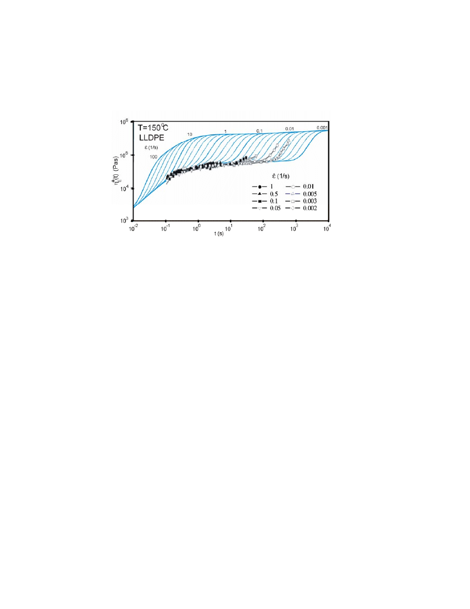
17

Measured and modelled elongational viscosities for LLDPE are shown in

Fig. 6. The stresses are orders of magnitude less than for LDPE in Fig.4. This

time we have used constant value for strain-hardening value P

H

as the data of

measurements at higher rates.

Figure 6. Measured and modelled elongational viscosities for LLDPE. The stresses are orders of

magnitude less than for LDPE in Fig. 4.

Comparison of Figs. 4 and 6 reveals that strain hardening has a greater

effect at higher elongation rates for LDPE and at lower elongation rates for

LLDPE. Several possible mechanisms could underlie the strain hardening of

LLDPE, including the presence of a few LCBs or components with high molar

masses, which are not detectable by classical analytical methods, and phase

separation in the molten state.

59

Strain hardening may peak at various times of

elongation measurements, which has been studied recently by Stadler et al..

30

Since the underlying mechanism remains somewhat obscure, we did not try to

model this feature but instead used the best fit with maximal strain hardening and

the same level for all elongation rates.

The next puzzle is the possibility of overshoot during elongation.

Rasmussen et al.

31

obtained an overshoot for LDPE Lupolen 1840 D, whereas

Burghelea et al.

32

argued that this phenomenon does not exist. This discrepancy is

why we present all of our simulation results as monotonically increasing without

an overshoot effect in charts for visual clarity; moreover, although the amount of

overshoot is not known, we still believe that some overshoot is present (as

discussed above).

In summary, the present measurements accurately provided the left side of

the effective hardening distribution RED

H

or LCBD, where this procedure is

18

sensitive to the results. The level of strain hardening was obtained by fitting

procedure.

Simulations of polymers with a high level of hardening

Polymers with a high level of hardening and LCB were simulated. For

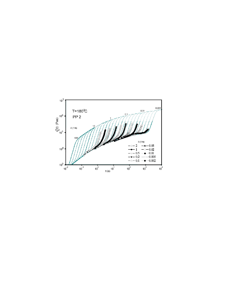
comparison we show a different chemical type of polymer in Fig. 7. The

simulated data were the measurements of the highly branched PP made by

Münstedt et al.

56

and used for all results for demonstration purposes constant

strain-hardening P

H

value, but uncertain results at higher elongations are dashed in

the figure.

Figure 7. Simulated results using Eq. (5) for highly branched PP according to measurements by

Münstedt et al.

56

(sample designated as PP 2 in that report). Strain hardening occurs over a wide

range of elongation rates. Since the measurements do not show any overshoot, a large-strain

approximation is used according to Eq. (5). We used constant strain-hardening P

H

to simulate

approximations in this case.

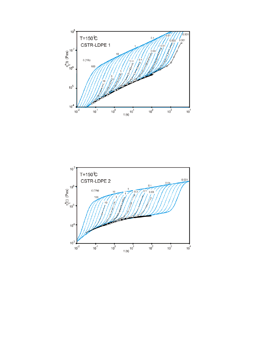
The last two presented simulations are of high-molecular-weight LDPEs

known to have a very high LCB content: (1) including many LCBs polymerized at

the laboratory scale in a continuously stirred tank reactor (CSTR) and (2) the

polymer designated as CSTR-LDPE 1. The results are shown in Fig. 8. We did

not know whether or not overshoot was present or the form of LCB distribution,

which is why we used Eq. (5) without the overshoot effect in the monotonically

increasing form for visual clarity (as discussed above). One novel interesting

feature of this simulation was that its results were consistent with the measured

strain-hardening spectrum for rates (i.e., values) of 0.1/s and 0.01/s, but not for

rates of =10/s and 0.001/s.

19

Figure 8. Simulated and measured spectra for CSTR-LDPE 1, with a high content of LCBs.

The results for another polymer, designated CSTR-LDPE 2 and which has

fewer LCBs, are shown in Fig. 9. The simulation results for this polymer were

consistent with the measured strain-hardening spectrum for all rates. Moreover,

the hardening effect was not as strong as in Fig. 8.

Figure 9. Simulated and measured spectra for CSTR-LDPE 2, with a lower content of LCBs.

Simulated MW-LCB distributions.

We generate long-chain branching distribution (LCBD) with MWD by

melt calibration Eq. (4) and by relation formula Eq. (8). RED

H

s were obtained by

a best-fit routine on a step-by-step basis based on the measurements and presented

formulas. During the procedure it was found that the results were very sensitive

even to the local forms of RED

H

s, which meant that we had to draw the final form

20

of the distribution curve manually in many cases. Since the shape of the LCB

distribution is the same on a logarithmic scale as the original RED

H

s, the results

provide valuable information on polymer structure and the constituent LCBDs.

We selected for conversions by melt calibration for

H

log , , where

=1/s. We depicted in Fig. 5 accurate RED- RED

H

s chart, now we present strain-

hardening distributions converted by melt calibration Eq. (4) to LCBD

H

) on M scale.

The

H

log , ) strain-hardening distributions are scaled by their strain-

hardening constant P

H

and respective main normalized MWDs in order to help

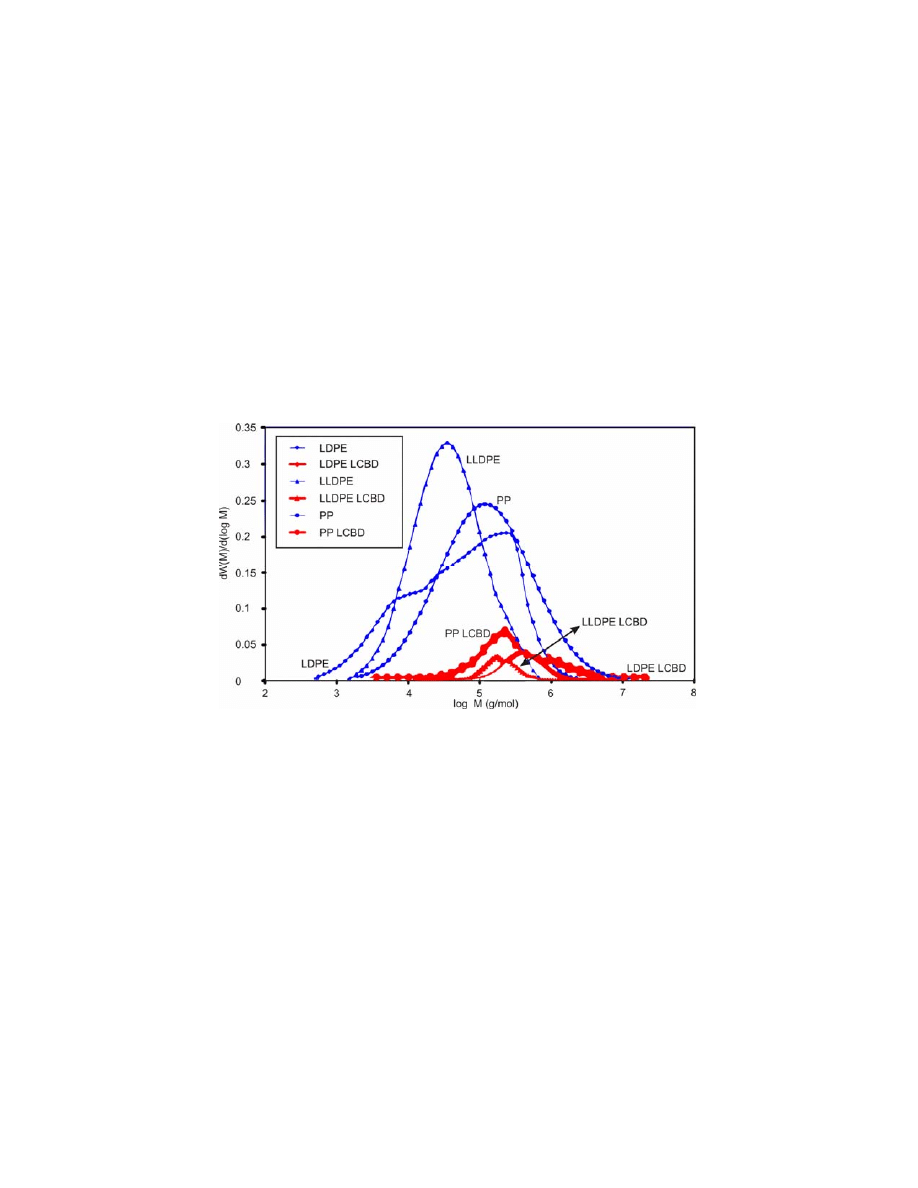
readers to evaluate the final bimodal MWD distributions in Figs. 10 and 11. Fig.

10 presents the MWDs and LCBDs used for commercial LDPE, LLDPE and PP.

Figure 10. The used MWDs and LCBDs, obtained from effective strain-hardening distribution

RED

H

or

H

log , ) by Eq. (8) for LDPE, LLDPE and PP simulations. Normalized MWD for

LLDPE and PP were extracted from GPC/SEC measurements and LDPE from RheoPower

database.

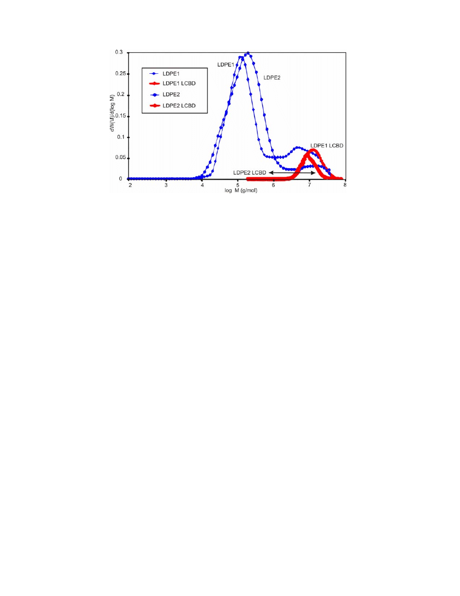
Fig. 11 depicts MWDs and LCBDs for LDPE formed at the laboratory

scale and containing a large amount of LCBs. The figure shows similarities with

data obtained by GPC/MALLS and the LCBs detected using our new method.

One interesting finding is that the PE polymer polydispersity of LCBDs

follows the polydispersity of the main MWDs, and also the PP spectrum appears

sharp.

21

Figure 11. The used MWDs and LCBDs, obtained from effective strain-hardening distribution

RED

H

or

H

log , ) by Eq. (8) for LDPE simulations. MWDs are from GPC/MALLS

measurements. Best-fit procedures revealed similarities between LCBDs as observed previously.

Conclusions

We have presented models and simulations of the elongational viscosity.

The obtained results indicate that the presented method is much more accurate at

detecting LCBs and even LCBDs than any other known method. However,

deeper studies involving more data must be performed in order to obtain the

correct Mf, Hf and P

H

values or even complete P

H

( ) function for the strain-

hardening distribution, which gives surely information of the inner backbone

segments. More research is also needed into the possibility of an overshoot effect

and its underlying mechanism, but this is not essential for detecting LCBs because

the present method is already able to detect about half of the complete LCBD.

We notice that single value for long chain branching frequency per 1000 C carbon

atoms (LCB/1000 C) is rather poor to describe branching although we had

opportunity to use LCBD as source data for computations.

The demonstrated properties represent only a small proportion of the

additional different applications for viscoelasticity and material analyses

obtainable from control theory. In practical manufacturing applications, this

elongation-based and (with LCBs) self-healing property is familiar, and it is

expected that future developments in measuring instruments will allow this

phenomenon to be fully described and analyzed.

22

The presented principles and multipurpose RheoPower software can be

used to simulate viscoelastic properties and material structures by generating

accurate linear relationships between them. Control theory avoids the need to

obtain the true absolute values, although the differences between the obtained

relative values must be accurate. This means that we can use not only shear or

dynamic viscosities or respectively the moduli or the elongational viscosity,

relaxation modulus or temperature, but also any (force-dependent) unit to obtain a

linear relation. Thus, the property variable can be the shear rate, frequency,

elongation rate, time, temperature or even, in principle, turns, rotations or

revolutions per second.

Moreover, macromolecules typically exhibit some distribution-dependent

behaviours, and thus the method is applicable to any material that is consistent

with the property of polydispersity, such as a collection of particles of any size,

objects or polymers that possess kinetic energy. Our novel melt calibration

principle makes it possible to find the real weight or size relating to the

viscoelasticity. The principle and software were originally developed for polymer

simulations, but the presented curves indicate that the technique can also be

flexibly applied in other rheological applications.

Used nomenclature:

P

Elastic

constant

Viscous

constant

H

Maximal

strain-hardening

constant

P

H

( )

Strain-hardening

variable

t

c

Characteristic time

Hencky

strain

Elongation

rate

,

Elongational viscosity at characteristic time t

c

= 1/s.

E

Elongational

viscosity without strain

hardening effect

E

Elongational viscosity including strain

hardening effect

Net tensile stress monitoring as a function of
time

LCBD, w

LCB

(M)

Long-chain branching distribution

MWD, w

MAIN

(M)

Molecular weight distribution obtained by
GPC/SEC

RED, w(log )

Rheologically effective distribution (elastic)

H

log )

Original strain-hardening component

23

RED

H

,

H

log , ) Effective

strain-hardening distribution as a

function of time and rate

χ(t, )

Strain-hardening

coefficient

References

1. Petrie CJS (2006) One hundred years of extensional flow, J Non-Newtonian Fluid Mech 137:

1–14

2. Mackley M (2010) Stretching polymer chains Rheol Acta 49: 443–458

3. Meissner J, Hostettler J (1994) A new elongational rheometer for polymer melts and other

highly viscoelastic liquids, Rheol Acta 33: 1–21

4. Laun HM, Schuch H (1989) Transient elongational viscosities and drawability of polymer

melts J Rheol 33:119–175

5. Münstedt H (1979) New universal extensional rheometer for polymer melts J Rheol 23: 421–

436

6. Münstedt H, Kurzbeck S, Egersdörfer L (1998) Influence of molecular structure on rheological

properties of polyethylenes Part II. Elongational behavior Rheol Acta 37: 21–29

7. Münstedt H, Steffl T, Malmberg A (2005) Correlation between rheological behaviour in

uniaxial elongation and film blowing properties of various polyethylenes Rheol Acta 45: 14–22

8. Sentmanat M (2004) Miniature universal testing platform: from extensional melt rheology to

solid-state deformation behaviour Rheol Acta 43: 657–669

9. Hassager O, Marin JMR, Yu K, Rasmussen HK (2010) Polymeric liquids in extension: fluid

mechanics or rheometry? Rheol Acta 49: 543–554

10. Aho J, Rolón-Garrido VH, Syrjälä S, Wagner MH (2010) Measurement technique and data

analysis of extensional viscosity for polymer melts by Sentmanat extensional rheometer (SER),

Rheol Acta 49: 359–370

11. van Ruymbeke E, Muliawan EB, Hatzikiriakos SG, Watanabe T, Hirao A, Vlassopoulos D

(2010) Viscoelasticity and extensional rheology of model Cayley-tree polymers of different

generations, J Rheol 54: 643–662.

12. Wagner MH (1979) Zur Netzwerktheorie von Polymer-Schmelzen Rheol Acta 18: 33–50

13. Wagner MH, Kheirandish S, Stange J, Münstedt H (2006) Modeling elongational viscosity of

blends of linear and long-chain branched polypropylenes, Rheol Acta 46: 211–221

14. Rolón-Garrido VH, Wagner M H (2007) The MSF model: relation of nonlinear parameters to

molecular structure of long-chain branched polymer melts Rheol Acta 46: 583–593

15. Rolón-Garrido VH, Pivokonsky R, Filip P, Zatloukal M, Wagner MH (2009) Modelling

elongational and shear rheology of two LDPE melts Rheol Acta 48: 691–697

16. Doi M, Edwards SFJ (1978) Dynamics of concentrated polymer systems. Part 2. Molecular

motion under flow J. Chem Soc, Faraday Trans 74: 1802–1817

24

17. Doi M, Edwards SFJ (1979) Dynamics of concentrated polymer systems. Part 4. Rheological

properties Chem Soc Faraday Trans 75: 38–54

18. Laun HM (1978) Description of the non-linear shear behaviour of a low density polyethylene

melt by means of an experimentally determined strain dependent memory function Rheol Acta 17:

1–15

19. Rauschenberger V, Laun HM (1997) A recursive model for Rheotens tests J Rheol 41: 719–

737

20. McLeish TCB, Larson RG (1998) Molecular constitutive equations for a class of branched

polymers: The pom-pom polymers J Rheol 42: 81–110

21. Inkson NJ, McLeish TCB, Harlen OG, Groves DJ (1999) Molecular constitutive equations for

a class of branched polymers: The pom-pom polymers J Rheol 43: 873–896

22. Likhtman AE, Graham RS (2003) Simple constitutive equation for linear polymer melts

derived from molecular theory: Roli-poly equation J Non-Newtonian Fluid Mech 114: 1–12

23. Auhl D, Chambon P, McLeish TCB, Read DJ (2009) Elongational Flow of Blends of Long

and Short Polymers: Effective Stretch Relaxation Time Phys Rev Lett 103:219801

24. van Ruymbeke, E Nielsen J, Hassager O (2010) Linear and nonlinear viscoelastic properties

of bidisperse linear polymers: Mixing law and tube pressure effect J Rheol 54: 1155–1172

25. Borg T, Pääkkönen EJ (2009) Linear viscoelastic models: Part I. Relaxation modulus and

melt calibration J Non-Newtonian Fluid Mech 156: 121–128

26. Borg T, Pääkkönen EJ (2009) Linear viscoelastic models: Part II. Recovery of the molecular

weight distribution using viscosity data J Non-Newtonian Fluid Mech 156: 129–138

27. Borg T, Pääkkönen EJ (2009) Linear viscoelastic models: Part III. Start-up and transient flow

effects from the molecular weight distribution J Non-Newtonian Fluid Mech 159: 17–25

28. Borg T, Pääkkönen EJ (2010) Linear viscoelastic models: Part IV. From molecular dynamics

to temperature and viscoelastic relations using control theory J Non-Newtonian Fluid Mech 165:

24–31

29. Kurzbeck S, Oster F, Münstedt H (1999) Rheological properties of two polypropylenes with

different molecular structure J Rheol 43: 359–374

30. Stadler FJ, Kaschta J, Münstedt H, Becker F, Buback M (2009) Influence of molar mass

distribution and long-chain branching on strain hardening of low density polyethylene, Rheol

Acta 48: 479–490

31. Rasmussen HK, Nielsen JK, Bach A, Hassager O (2005) Viscosity overshoot in the start-up of

uniaxial elongation of low density polyethylene melts, J Rheol 49: 369–381

32. Burghelea TI, Starý Z, Münstedt H (2011) On the "viscosity maximum" during the uniaxial

extension of a low density polyethylene J Non-Newtonian Fluid Mech 166: 1198–1209

33. Fleury G, Schlatter G, Muller R (2004) Non Linear Rheology for Long Chain Branching

characterization, comparison of two methodologies: Fourier Transform Rheology and Relaxation

Rheol Acta 44: 174–187

25

34. Malmberg A, Gabriel C, Steffl T, Münstedt H, Löfgren B (2002) Long-chain branching in

metallocene-catalyzed polyethylenes investigated by low oscillatory shear and uniaxial extensional

rheometry Macromolecules 35: 1038–1048

35. Costeux S (2003) Modeling of Randomly Branched Polymers Produced by Combination of

Several Single-Site Catalysts: Toward Optimization of Melt Properties Macromolecules 36: 4168–

4187

36. Chen X, Costeux C, Larson RG (2010) Characterization and prediction of long-chain

branching in commercial polyethylenes by a combination of rheology and modeling methods J

Rheol 54: 1185–1206

37. Wood-Adams PM, Dealy JM, deGroot AW, Redwine OD (2000) Effect of Molecular

Structure on the Linear Viscoelastic Behavior of Polyethylene Macromolecules 33: 7489–7499

38. Sugimoto M, Suzuki Y, Hyun K, Ahn KH, Ushioda T, Nishioka A, Taniguchi T, Koyama K

(2006) Melt rheology of long-chain-branched Polypropylenes Rheol Acta 46: 33–44

39. Vega JF, Expósito MT, Martínez-Salazar J, Lobón-Poo M, Barcina JO, Martínez AG, López

M (2011) Molecular architecture and linear viscoelasticity of homogeneous ethylene/styrene

copolymers Rheol Acta 50:207–220

40. Zimm BH, Stockmayer WH (1949) The dimensions of chain molecules containing branches

and rings J Chem Phys 17:1301–1314

41. Vega JF, Fernándes M, Santamariá A, Muñoz-Escalona A, Lafuente P (1999) Rheological

criteria to characterize metallocene catalyzed polyethylenes Macromol Chem Phys 200: 2257–

2268

42. Gabriel C, Kokko E, Löfgren B, Seppälä J, Münstedt H (2002) Analytical and rheological

characterization of long-chain branched metallocene-catalyzed ethylene homopolymers Polymer

43: 6383–6390

43. Malmberg A, Liimatta J, Lehtinen A, Löfgren B (1999) Characteristics of long chain

branching in ethene polymerization with single site catalysts Macromolecules 32: 6687–6696

44. Malmberg A, Kokko E, Lehmus P, Löfgren B, Seppälä J (1998) Long-chain branched

polyethene polymerized by metallocene catalysts Et[Ind]2ZrCl2/MAO and

Et[IndH4]2ZrCl2/MAO Macromolecules 31: 8448–8454

45. Wood-Adams PM, Dealy JM (2000) Using rheological data to determine the branching level

in metallocene polyethylenes Macromolecules 33: 7481–7488

46. Gabriel C, Münstedt H (2002) Influence of long-chain branches in polyethylenes on linear

viscoelastic flow properties in shear Rheol Acta 41: 232–244

47. van Gurp M, Palmen J (1998) Time temperature superposition of polymeric blends Rheol Bull

67: 5–8

48. Trinkle S, Walter P, Friedrich C (2002) Van Gurp–Palmen Plot II—classification of long

chain branched polymers by their topology Rheol Acta 41: 103–113

49. García-Franco CA, Srinivas S, Lohse DJ, Brant P (2001) Similarities between gelation and

long chain branching viscoelastic behavior Macromolecules 34: 3115–3117

26

50. Keßner U, Kaschta J, Münstedt H (2009) Determination of method-invariant activation

energies of long-chain branched low-density polyethylenes J Rheol 53: 1001–1016

51. Keßner U, Kaschta J, Stadler FJ, Le Duff CS, Drooghaag X, Münstedt H (2010)

Thermorheological Behavior of Various Short- and Long-Chain Branched Polyethylenes and Their

Correlations with the Molecular Structure, Macromolecules, 43: 7341–7350

52. Soares JBP, Hamielec AE Bivariate (1996) Chain Length and Long Chain Branching

Distribution for Copolymerization of Olefins and Polyolefin Chains Containing Terminal Double

Bonds Theory Simul 5: 547–572

53. Meimaroglou D, Krallis A, Saliakas V, Kiparissides C (2007) Macromolecules 40: 2224–2234

54. Meimaroglou D, Kiparissides C 2010 Macromolecules 43: 5820–5832

55. Costeux S, Wood-Adams P, Beigzadeh D (2002) Molecular Structure of Metallocene-

Catalyzed Polyethylene: Rheologically Relevant Representation of Branching Architecture in

Single Catalyst and Blended Systems Macromolecules 35: 2514–2528

56. Münstedt H, Kurzbeck S, Stange J (2006) Importance of Elongational Properties of Polymer

Melts for Film Blowing and Thermoforming Polym Eng Sci 46: 1190–1195

57. Borg T (Muolon Oy) Method of producing a shrinkable product U.S. Patent 5,053,174,

October 1 1991

58. Starý Z, Münstedt H (2008) Morphology Development in PS/LLDPE Blend During and After

Elongational Deformation J Polym Sci Part B: Polym Phys 46: 16–27

59. Lohse DJ, Milner ST, Fetters LJ, Xenidou M, Hadjichristidis N, Menedelson RA, Garcia-

Franco CA, Lyon MK (2002) Well-Defined, Model Long Chain Branched Polyethylene. 2. Melt

Rheological Behavior, Macromolecules 35: 3066–3075