Page

1

ANSYS Tutorials

Grady Lemoine

Table of Contents

Example 1: 2-D Static Stress Analysis in ANSYS..............................................2

Example 2: 3-D Static Stress Analysis ................................................................5

Example 3: 2-D Frame With Multiple Materials and Element Types...............10

Example 4: 3-D Truss ........................................................................................15

Example 5: Simple 2-D Heat Transfer ..............................................................20

Example 6: Modal Analysis...............................................................................22

Example 7: Plate Buckling Analysis Part 1: Eigenvalue Buckling Analysis....26

Example 8: Plate Buckling Analysis Part 2: Nonlinear Buckling Analysis......31

Example 9: Simple Dynamic Analysis ..............................................................35

Example 10: Box Beam .....................................................................................39

Page

2

Example 1: 2-D Static Stress Analysis in ANSYS

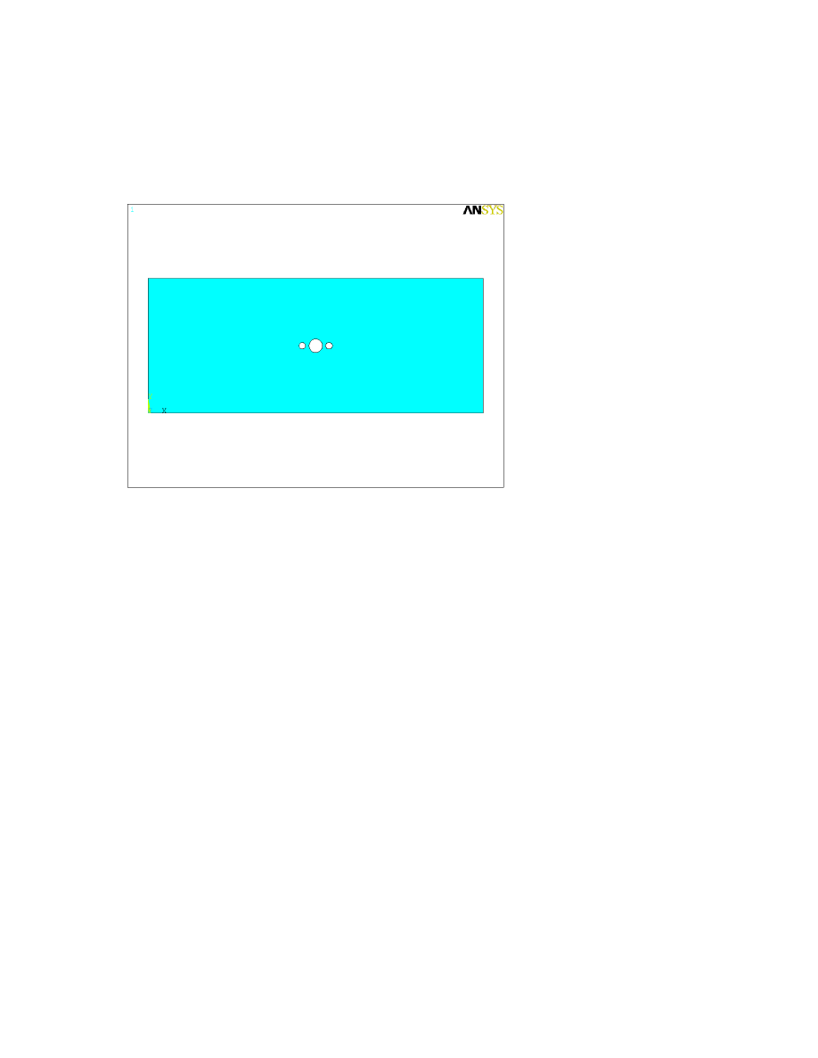
In this example we will examine the stress concentrations in a flat plate with three holes, as shown in
Figure 1.1.

Figure 1.1

Preprocessor

First, we will select an element type, define element and material properties, create a model, and mesh it in
the Preprocessor.

Selecting an element type:

1. Click on ‘Preprocessor’ in the ANSYS main menu at the left side of the screen.

2. Click on ‘Element Type->Add/Edit/Delete’.

3. Click ‘Add’.

4. Choose ‘Solid’ from the ‘Structural’ list of element types, then ‘Quad 4node 42’ from the list on the
right. This chooses a four-node quadrilateral 2D element.

5. Click ‘OK’, then click ‘Close’ on the Element Types box and close the Element Types menu.

Defining material properties:

1. Click ‘Material Props’ in the Preprocessor menu.

2. Click ‘Material Models’.

3. Double-click ‘Structural’ in the right side of the window, then ‘Linear’, then ‘Elastic’, then finally
‘Isotropic’.

Page

3

4. Enter in values for Young’s modulus and Poisson’s ratio. In this problem we use a Young’s modulus of
70e9 and a Poisson’s ratio or 0.3, which are ballpark values for aluminum (note that ANSYS understands
scientific “e” notation). No other material properties will be needed, so click ‘OK’, then close the Material
Properties menu.

Creating a model:

1. Click ‘Create’ under the ‘-Modeling-‘ heading on the Preprocessor menu.

2. First create the rectangle for the plate. Under the ‘-Areas-‘ heading click ‘Rectangle’, then ‘By
Dimensions’ on the menu that pops up.

3. Put 0 and 0.5 in the X1,X2 boxes and 0 and 0.2 in the Y1,Y2 boxes. This will create a rectangle with
corners at (0,0) and (0.5,0.2).

4. Now create the circles for the holes. Under the ‘-Areas-‘ heading click Circle, then ‘Solid Circle’ on the
resulting menu.

5. Create the circles by entering the X and Y coordinates in the boxes marked ‘WP X’ and ‘WP Y’ and the
radius in the box marked ‘Radius’. (You can also create circles by clicking in the graphics window, but this
method cannot discriminate finely enough to be usable here.) Enter in the following for the circles, clicking
‘Apply’ after each one.

WP X

WP Y

Radius

Circle 1

0.25

0.1

0.01

Circle 2

0.23

0.1

0.005

Circle 3

0.27

0.1

0.005

6. Now you are done creating areas and can subtract the circles from the rectangle to create the desired
plate with holes. Close the ‘Create’ menu, and click ‘Operate’ under the ‘-Modeling-‘ heading on the
Preprocessor menu.

7. Click ‘Subtract’ under the ‘-Booleans-‘ heading, then click ‘Areas’.

8. First click the area you want to subtract from (the rectangle in this case). The selected area will change
color. If you select the wrong area, you can unpick it by right-clicking to switch unpick mode, then clicking
it again (you can then switch back to pick mode by right-clicking again). Be sure that the entire area and
only the area you want to subtract from is highlighted. When you are done, click ‘OK’.

9. Now select the areas you want to subtract. Click each of the circles, then click ‘OK’. (When clicking the
center circle you will get a message saying that there is more than one area at the location you selected.
Click ‘Next’ until the circle is highlighted.) You will now have a rectangle with three holes, and have
finished creating your model.

Meshing the model:

1. On the Preprocessor menu, click ‘MeshTool’.

2. Select the size of your mesh. In this case we will use the Smart Size feature to choose an appropriate size
automatically. Click the Smart Size pinpoint and use the slider to set the size setting to 5. (When working
through a new problem, it’s always best to use a fairly coarse mesh to begin with since it will be faster to
solve and use less disk space.)

3. Leave the rest of the settings at their defaults and click ‘MESH’. Click on the plate, then click ‘OK’ in
the input box at the lower left of the screen.

Page

4

4. Since we expect large stress gradients around the holes, we’ll want to refine the mesh around them. Click
the box next to the word ‘Refine’ and select ‘at Lines’, then click the ‘Refine’ button below it.

5. Click on the edges of each hole (you will need to click once for each quadrant of each circle), then click
‘OK’. Leave the settings at their defaults in the ‘Refine Mesh at Line’ box that appears, and click ‘OK’.
ANSYS will refine the elements in the region of the holes.

6. You are now done meshing. Click ‘Close’ in the MeshTool box.

Solution

Next, we set up an analysis, define displacements and loadings, and solve the problem.

Setting up an analysis:

1. Click on ‘Solution’ in the ANSYS main menu.

2. Click on ‘New Analysis’ under the ‘-Analysis Type-‘ heading. ‘Static’, the type desired for this problem,
will be the default; if it is not selected, select it. Then click ‘OK’.

Fixing the left edge of the plate:

1. Click on ‘Apply’ under the ‘-Loads-‘ heading.

2. Click ‘Displacement’, then ‘On Lines’.

3. Click on the left edge of the plate, then click ‘OK’.

4. Click ‘UX’ in the box listing degrees of freedom (DOFs) to be constrained, then enter 0 into the
displacement value box.

5. Click ‘OK’, then close the Displacement menu.

Applying a stress to the right edge of the plate:

1. Click ‘Pressure’ on the Apply Loads menu, then click ‘On Lines’. (All distributed surface forces come
under the heading of pressure in ANSYS).

2. Click the right edge of the plate, then click ‘OK’ and enter -1e6 in the upper ‘VALUE’ box. This will
apply a stress of 1 megapascal, in tension (positive values correspond to compression, negative to tension).
Click ‘OK’ to apply the load.

3. Close the Apply Loads menu.

Solving the problem:

1. Under the ‘-Solve-‘ heading, click ‘Current LS’. This will solve the current “Load Step”. Review the
information in the window that appears to see if everything is in order, then click ‘OK’ (or ‘Cancel’ to
cancel solution).

Postprocessor

Finally we use the Postprocessor to display the results.

1. Click ‘General Postproc’ on the ANSYS main menu.

Page

5

2. Click ‘Plot Results’.

3. Under the ‘-Contour Plot-‘ heading, click ‘Nodal Solu’.

4. Choose the quantity you wish to see displayed. In this case, pick ‘Stress’ from the box on the left, and
‘1

st

principal S1’ from the one on the right to plot the first principal stress.

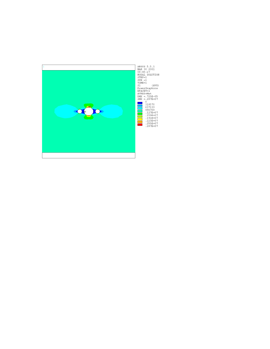
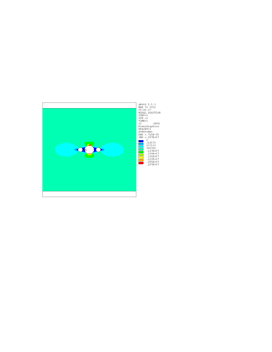
ANSYS marks the locations of the maximum and minimum values of the quantities plotted with ‘MX’ and
‘MN’ on the plot. Note that the maximum stress occurs at the top (and bottom) of the center hole and the
minimum occurs between the holes. The maximum stress is also shown at the right side of the plot window
as ‘SMX’.

A close-up of the contour plot in the region of the holes is shown in Figure 1.2.

Figure 1.2

Example 2: 3-D Static Stress Analysis

In this example we will examine the stresses in a large isotropic block subjected to a point load and fixed at
the bottom. By symmetry, we can model the entire block using only one quadrant and specifying zero
displacement on two of the faces. We will use English units of feet and pounds for this problem.

Preprocessor

Select an element type:

1. Click on ‘Preprocessor’ in the ANSYS main menu at the left side of the screen.

2. Click on ‘Element Type->Add/Edit/Delete’.

3. Click ‘Add’.

4. Choose ‘Solid’ from the ‘Structural’ list of element types, then ‘Brick 8node 45’ from the list on the right
(you will need to scroll down). This chooses a rectangular solid element with a node at each corner.

Page

6

5. Click ‘OK’, then click ‘Close’ on the Element Types box and close the Element Types menu.

Defining material properties:

1. Click ‘Material Props’ in the Preprocessor menu.

2. Click ‘Material Models’.

3. Double-click ‘Structural’ in the right side of the window, then ‘Linear’, then ‘Elastic’, then finally
‘Isotropic’.

2. Enter in values for Young’s modulus and Poisson’s ratio. In this problem we use a Young’s modulus of
144e7 and a Poisson’s ratio of 0.34, which are ballpark values for aluminum in English units (the Young’s
modulus has been converted from lb/in2 to lb/ft2). No other material properties will be needed, so click
‘OK’, then close the Material Properties menu.

Creating a model:

1. Click ‘Create’ under the ‘-Modeling-‘ heading on the Preprocessor menu.

2. Create the block by clicking ‘Block’ under the ‘-Volumes-‘ heading, then clicking ‘By Dimensions’.

3. Enter the following coordinates in the input boxes:

X1,X2

0

10

Y1,Y2

0

10

Z1,Z2

0

10

This will create a block with one corner at the origin and the opposite corner at (10,10,10) feet. The load
will be applied to the corner at (0,0,10).

Now close the ‘Block’ and ‘Create’ menus.

At this point you will need to be able to rotate the graphical display so that you can access all the edges of
the quarter-block. To do this, click the ‘PlotCtrls’ menu at the top of the screen, then click
‘Pan/Zoom/Rotate’ and use the buttons marked with a curving arrow and ‘+X’, ‘-Y’, etc., to rotate the plot.
When you are done, click ‘Close’ on the box. Note that you can use the Pan/Zoom/Rotate box while you
are doing other tasks such as picking objects for an input box.

Meshing the model:

1. On the Preprocessor menu, click ‘MeshTool’.

2. This time we will define the size variations of the elements manually. On the ‘Plot’ menu at the top of
the screen, click ‘Lines’ to show only the currently defined lines (the edges of the quarter-block). Next,
under the ‘Lines’ subheading of the ‘Size Controls’ part of the MeshTool box, click ‘Set’. This will set the
size and division spacing ratio along the lines you choose.

3. Click ‘Pick All’.

4. Enter 4 in the ‘No. of element divisions’ box and 3 in the ‘Spacing ratio’ box. This chooses four
divisions along the line, with the last three times as long as the first. (Choosing a coarse mesh at first is
especially important for 3-D problems since the total number of elements goes up as the cube of the
number of elements on a side rather than the square. A fine mesh can take a very long time to solve.)

Page

7

5. Now all the lines will have the correct number of divisions and spacing ratio, but not all of them will
have their smallest elements oriented toward the corner at (0,0,10) where the load will be applied. To flip
the orientations of those that don’t point in the correct direction, click ‘Flip’ on under the ‘Lines’
subsection of the MeshTool box.

6. Pick all the lines that do not have their shortest elements oriented toward (0,0,10), then click ‘OK’ to flip
their orientations.

7. Now click ‘Hex’ next to ‘Shape’ on the MeshTool box. This will use brick (six-sided) elements rather
than tetrahedral elements, as is the default. When you choose ‘Hex’, the mesher type (shown below the
shape type) will automatically change to ‘Map’, which will use the divisions of the lines to define (“map”)
the mesh.

8. Click ‘Mesh’, then click on the quarter-block and click ‘OK’ to create the mesh. If the mesh does not
come out right, you can repeat steps 2-8 to re-form it.

9. You are now done meshing and have finished with the Preprocessor. Click ‘Close’ on the MeshTool box,
then close the Preprocessor menu.

Solution

Now we go to the Solution step to set up the analysis, define loadings, and solve the problem.

Setting up the analysis:

1. Click on ‘Solution’ on the ANSYS main menu.

2. Click on ‘New Analysis’ under the ‘-Analysis Type-‘ heading. ‘Static’, the type desired for this problem,
will be the default; if it is not selected, choose it. Then click ‘OK’.

Applying the load:

1. Under the ‘-Loads-‘ heading on the ‘Solution’ menu, click ‘Apply’.

2. Click ‘Force/Moment’.

3. Click ‘On Nodes’.

4. Click the corner of the quarter-block at (0,0,10), then click ‘OK’ in the pick box.

5. Click on the box labeled ‘Direction of force/mom’, then click ‘FZ’.

6. Enter a value of -45*2000/4 in the box labeled ‘Force/moment value’, then click ‘OK’. This applies one
quarter of a 45-ton load downward on the quarter-block.

Applying displacements:

The quarter-block will be fixed at the bottom. In addition, since the whole block can be thought of as four
of the quarter-blocks we’re analyzing placed face-to-face, we know that the faces of the quarter-block in
the XZ and YZ planes will have no displacement perpendicular to their surfaces, since if they did that
would indicate voids in the full block (where the quarter-block faces displace inward) or places where
material pushes through other material (where the faces displace outward).

1. Click ‘Displacement’ on the ‘Apply’ menu.

2. Click ‘On Areas’.

Page

8

3. Click on the face of the quarter-block in the YZ plane (facing in the negative X direction), then click
‘OK’ in the pick box. If that face is not visible, you can use the Pan/Zoom/Rotate function to rotate the
model until it is.

4. Select ‘UX’ as the degree of freedom to be constrained, then enter a displacement value of 0 and click
‘OK’.

5. Click ‘On Areas’ again, then select the face of the quarter-block in the XZ plane (facing in the negative
Y direction) and apply a ‘UY’ displacement of 0.

6. Click ‘On Areas’ again, then this time select the bottom of the quarter-block, choose ‘All DOF’ to be
constrained, and enter a displacement value of 0.

7. You have now finished applying loads. Close the ‘Displacement’ and ‘Apply’ menus.

Solving the problem:

1. Under the ‘-Solve-‘ heading, click ‘Current LS’. Review the information in the window that appears to
see if everything is in order, then click ‘OK’ (or ‘Cancel’ to cancel solution).

Postprocessor

Finally, we view the results.

1. Click ‘General Postproc’ on the ANSYS main menu.

2. Click ‘Plot Results’.

3. Under the ‘-Contour Plot-‘ heading, click ‘Nodal Solu’.

4. Choose the quantity you wish to see displayed. In this case, pick ‘Stress’ from the box on the left, and
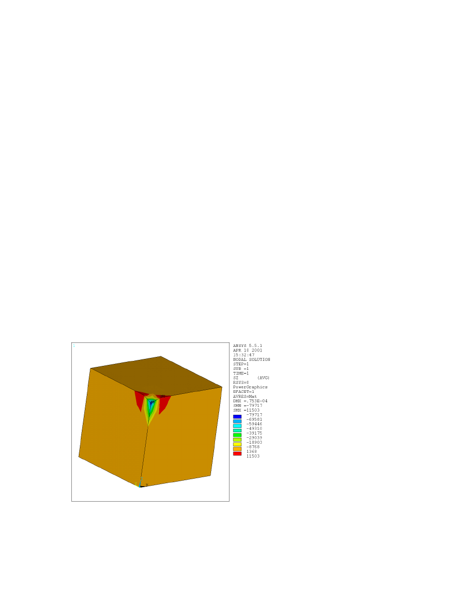
‘Z-direction SZ’ from the box on the right to display the normal stress in the Z direction. The resulting plot
is shown in Figure 2.1.

Figure 2.1

The regions of tensile stress near the load are artifacts of the mesh.

Page

9

We can also define “paths” (sequences of elements through the model) and graph the results along these:

1. On the General Postprocessor menu, click ‘Path Operations’ (about 2/3 of the way down the list).

2. Click ‘Define Path’.

3. Click ‘By Nodes’.

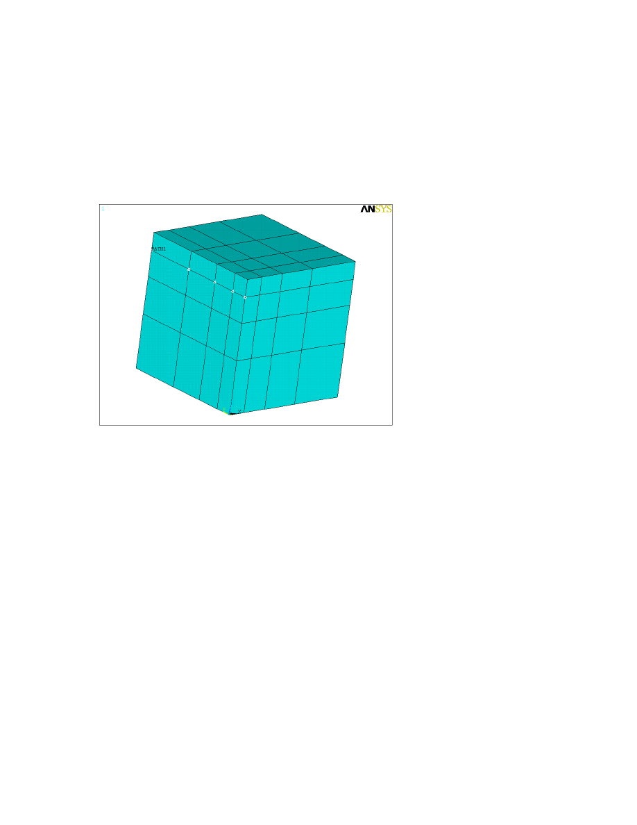
4. Click the second tier of nodes in the YZ plane, as shown in Figure 2.2, then click ‘OK’. (Figure 2.2 was
produced using the ‘Plot Paths’ function in ANSYS.)

Figure 2.2

5. Enter a name for the path in the box labeled ‘Define Path Name’, then click ‘OK’. A window will appear
showing the locations and numbers of the nodes on the path.

6. Click ‘Map onto Path’ to transfer data from your solution to the path.

7. Choose the Z-direction stress (‘Stress’ in the left box and ‘Z-direction SZ’ in the right), then click ‘OK’.

8. Under the ‘-Plot Path Item-‘ heading, click ‘On Graph’.

9. Choose ‘SZ’, then click ‘OK’.

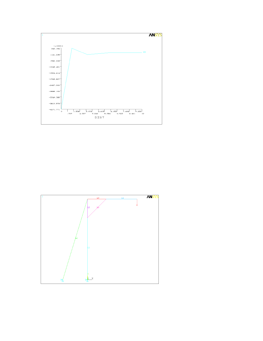
The resulting plot is shown in Figure 2.3.

Page

10

Figure 2.3

Example 3: 2-D Frame With Multiple Materials and Element
Types

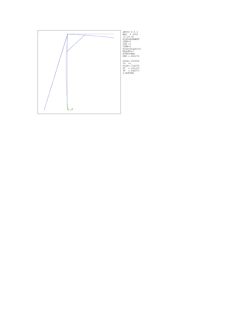
In this example we will find the loads and stresses in a two-dimensional frame with members made of
different materials and having different cross-sections. The frame is shown in Figure 3.1. Members 1, 2, 3,
4, and 5 are aluminum beams and have a hollow square cross-section with outer wall size 2 cm and wall
thickness 2 mm, and member 6 is a steel wire with diameter 2 mm. The applied force is 100 N.

Figure 3.1

Page

11

Preprocessor

First, we will select element types, define element and material properties, define a model, and mesh it.

Element types:

Member 5 is a two-force member, so it will support only an axial force and can be most economically
modeled as a 2D spar element, which only resists axial force. Member 6 is also a two-force member, so it
will be modeled as a 2D spar as well. (A tension-only spar is available, but it is a 3D element and we would
like to keep this a strictly 2D problem.) Members 1, 2, 3, and 4 will need to support a moment, so they
should be modeled as 2D beam elements.

1. On the ANSYS main menu, click ‘Preprocessor’.

2. Click ‘Element Type’.

3. Click ‘Add/Edit/Delete’, then ‘Add’ on the box that appears.

4. Choose ‘Beam’ under the Structural heading in the left box, then ‘2D elastic 3’ in the right box to select
the 2D beam element, then click ‘Apply’.

5. Click ‘Link’ under the Structural heading in the left box, then ‘2D spar 1’ in the right box to select the
2D spar (two-force member) element. Then click ‘OK’. You have defined the element types needed for this
problem.

Real constants:

Now you can define cross-sectional areas and second area moments for the members using “real constant”
sets. From the ANSYS online help, “real constants are properties that depend on the element type, such as
cross-sectional properties of a beam element”.

1. On the Preprocessor menu, click ‘Real Constants...’.

2. Click ‘Add’.

3. Click ‘Type 1 BEAM3’, then click ‘OK’ to choose to define a real constant set for the beam elements.
Note that there is not a one-to-one correspondence between real constant sets and element types—you can
have more than one real constant set for each element type, and ANSYS keeps track of real constants and
element types independently.

4. The cross-sectional area and second area moment of the beam are 1.44 cm2 and 0.7872 cm4 respectively
(you can verify this yourself). To aid in keeping consistent units throughout the analysis, we’ll enter these
in terms of meters. Enter 1.44e-4 in the box marked ‘Cross-sectional area’, 0.7872e-8 in the box marked
‘Area moment of inertia’, and 2e-2 (2 cm) in the box marked ‘Total beam height’, then click ‘OK’.

5. Now click ‘Add’ again in the Real Constants box, then choose ‘Type 2 LINK1’ and click ‘OK’.

6. This time we will define constants for member 5, the two-force hollow aluminum member. In the box
marked ‘Cross-sectional area’ enter 1.44e-4 and click ‘OK’.

7. Finally, we will define real constants for the steel wire. Click ‘Add’ once more in the Real Constants
box, then choose ‘Type 2 LINK1’ and click ‘OK’.

8. Enter 3.14159*(1e-3**2) in the box marked ‘Cross-sectional area’. (The radius of the wire is 1 mm. Note
that ANSYS uses “**” for exponentiation as in FORTRAN, rather than “^” as in BASIC and most
programmable calculators.) Then click ‘OK’. You have now finished defining real constants; click ‘Close’
in the Real Constants box.

Page

12

Next we will define material properties.

Defining material properties:

1. Click ‘Material Props’ in the Preprocessor menu.

2. Click ‘Material Models’.

3. Double-click ‘Structural’ in the right side of the window, then ‘Linear’, then ‘Elastic’, then finally
‘Isotropic’.

4. Enter 70e9 (70 GPa) in the box for Young’s modulus (“EX”) and 0.3 in the box for ‘Poisson’s ratio’
(“PRXY”), then click ‘Apply’. (These are ballpark values for aluminum.)

5. Click ‘New Model’ on the ‘Material’ menu in the Define Material Model Behavior window.

6. Set the material ID to 2, then click ‘OK’.

7. Double-click ‘Isotropic’ again, enter 210e9 (210 GPa) in the Young’s modulus box, then click ‘OK’.
(This is a ballpark value for steel; we don’t need to enter Poisson’s ratio since all the steel objects in the
frame are loaded uniaxially.) You have finished defining material properties.

Now we will create our model of the frame.

Creating the model:

1. Under the ‘-Modeling-‘ heading on the Preprocessor menu, click ‘Create’.

2. Click ‘Keypoints’.

3. Click ‘In Active CS’.

4. Create the following keypoints, clicking ‘Apply’ after entering in the values for each one:

Keypoint number

X

Y

1

0

0

2

0

1

3

0

1.3

4

0.3

1.3

5

0.8

1.3

6

-0.4

0

Then click ‘OK’ to close the Create Keypoints in Active Coordinate System box, and close the Keypoints
menu.

5. Under the ‘-Lines-‘ heading click ‘Lines’.

6. Click ‘In Active Coord’.

7. You can now create lines by clicking on their endpoints, then clicking ‘OK’ or ‘Apply’ in the Lines in
Active Coord box. Create lines between keypoints 1 and 2, 2 and 3, 3 and 4, 4 and 5, 2 and 4, and 3 and 6,
then click ‘OK’. (Note that keypoint 1 coincides with the origin.) You have now finished creating the
geometry model for the problem; close the Lines and Create menus.

Page

13

We will now specify what material, element type, and real constant set to use with each line by defining
element attributes.

Defining element attributes:

1. Under the ‘-Attributes-‘ heading on the Preprocessor menu, click ‘Define’.

2. Click ‘Picked Lines’.

3. Click the lines between keypoints 1 and 2, 2 and 3, 3 and 4, and 4 and 5, then click ‘OK’.

4. In the box that appears, choose material number 1 (defined earlier as aluminum), real constant set 1
(defined for the beam elements), and element type 1 (the 2D beam element), then click ‘OK’. (These
should be the defaults anyway.)

5. Click ‘Picked Lines’ again, and choose the line between keypoints 2 and 4. Assign this line material
number 1, real constant set 2 (for the hollow aluminum members treated as spars), and element type 2 (the
2D link).

6. Click ‘Picked Lines’ a third time and choose the line between keypoints 3 and 6. Assign this line
material number 2 (steel), real constant set 3 (for the steel wire), and element type 2. You are now done
defining attributes; close the Define menu.

Finally we will mesh the model.

Meshing:

1. On the Preprocessor menu, click ‘MeshTool’.

2. First we will set element sizes on the lines. Next to ‘Lines’ under the ‘Size Controls’ heading, click ‘Set’.

3. Pick the lines between keypoints 1 and 2, 2 and 3, 3 and 4, and 4 and 5, then click ‘OK’.

4. Enter 0.1 in the element edge length box, then click ‘OK’. This requests that the lines be divided into
elements (beam elements in this case) 0.1 meter long. Note that ANSYS would give accurate results even if
we used only one element per line; we are using more only to get an idea of the deformed shape.

2. Click ‘Set’ for the line size controls again, and pick the two remaining lines (keypoints 2-4 and 3-6), then
click ‘OK’.

3. Clear the element size box and set the number of element divisions to 1, then click ‘OK’. (Since these
members will remain straight, there is no point in using more elements; in fact, using more would be
detrimental in this case.)

4. Click ‘MESH’ at the bottom of the MeshTool box, then click ‘Pick All’ in the pick box to mesh all of the
lines. You have now created your mesh; close the MeshTool.

You have finished with the preprocessor; close the Preprocessor menu.

Solution

Now we will define the loads and displacements and solve the problem:

Defining displacements:

1. Click ‘Solution’ on the ANSYS main menu.

Page

14

2. Under the ‘-Loads-‘ heading, click ‘Apply’. (We don’t need to explicitly define an analysis type here
since the type we want, Static, is the default.)

3. Click ‘Displacement’.

4. Click ‘On Keypoints’.

5. Click the bottom of the vertical portion of the frame and the lower end of the wire (keypoints 1 and 6),
then click ‘OK’.

6. Click ‘UX’ and ‘UY’ in the box that appears, and enter 0 in the box marked ‘Displacement value’, then
click ‘OK’. This applies simple support (rotation allowed but no translation) to both selected points. You
are now done defining displacements. Close the Displacement menu.

Defining loads:

1. Click ‘Force/Moment’ on the Apply menu.

2. Click ‘On Keypoints’.

3. Pick the end of the horizontal member of the frame (keypoint 5), then click ‘OK’.

4. Select ‘FY’ from the box marked ‘Direction of force/moment’, then enter -100 in the ‘Force/moment
value’ box and click ‘OK’. This defines a 100 N force downward on the end of the horizontal member.

Solving the problem:

1. On the Solution menu, under the ‘-Solve-‘ heading click ‘Current LS’. Review the information summary
box that appears, and if everything appears to be in order click ‘OK’. ANSYS will now solve the problem.

Postprocessor

Finally, we can view and list the results in the Postprocessor:

1. Click ‘General Postprocessor’ on the ANSYS main menu.

To plot the deformed shape of the frame:

1. Click ‘Plot Results’ on the General Postprocessor menu.

2. Click ‘Deformed shape’.

3. Choose ‘Def shape only’, ‘Def + undeformed’, or ‘Def + undef edge’, depending on whether you want to
see the deformed shape alone or with the undeformed shape as well. A plot of the deformed shape with the
undeformed shape’s edge is shown in Figure 3.2.

Page

15

Figure 3.2

To list the stresses in the elements as well as other element data:

1. Click ‘List Results’ on the General Postprocessor menu.

2. Click ‘Element Solution’.

3. Choose ‘LineElem Results’ in the left box, and ‘Structural’ in the right, then click ‘OK’.

The results in the window that appears can also be printed out or saved to a file from the ‘File’ menu in that
window.

To list the forces at each node, repeat the above procedure but choose ‘Nodal force data’ in the left box.

To list the reactions at the supports:

1. On the List Results menu, click ‘Reaction Solu’.

2. Choose the types of reactions you wish to see and click ‘OK’.

Example 4: 3-D Truss

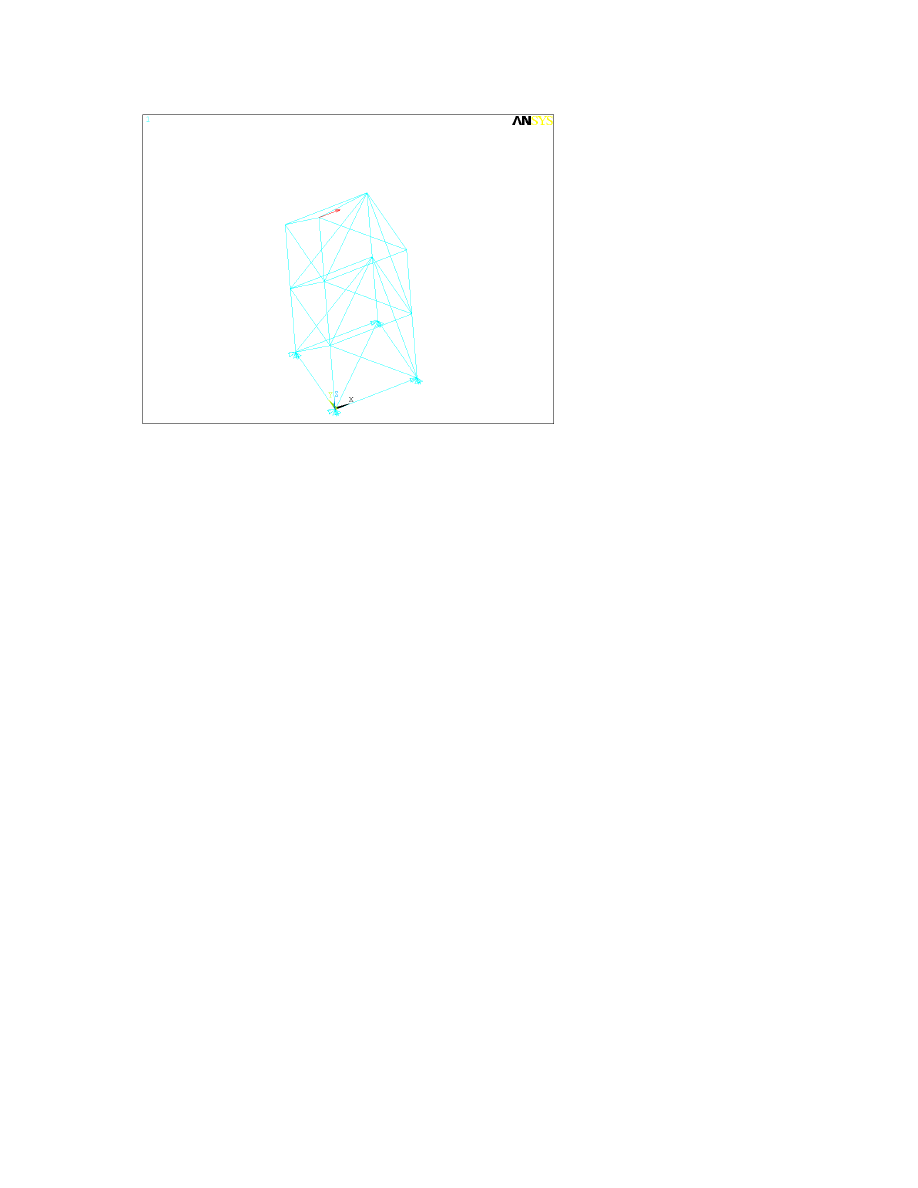
In this example we will solve for the member forces and deflections of an elastic three-dimensional truss,
shown in Figure 4.1.

Page

16

Figure 4.1

Preprocessor

First we will select an element type, define element and material properties, and define nodes and elements:

Selecting an element type:

1. On the Preprocessor menu, click ‘Element Type’.

2. Click ‘Add/Edit/Delete’.

3. Click ‘Add’.

4. Choose ‘Link’ in the left box and ‘3D spar 8’ in the right, then click ‘OK’. This selects the 3D spar (two-
force member) element.

Defining real constants:

For this problem we will use inches as our distance units and pounds for our force units.

1. On the Preprocessor menu, click ‘Real Constants’.

2. Click ‘Add’, then ‘OK’ in the box that appears.

3. Enter 1 (1 square inch) in the box marked ‘Cross-sectional area’. All the members will have this cross-
sectional area, so only one real constant set is needed. Now click ‘OK’ and close the Real Constants box.

Defining material properties:

1. Click ‘Material Props’ on the Preprocessor menu.

2. Click ‘Material Models’, then click ‘OK’.

3. Double-click ‘Structural’ in the right side of the window, then ‘Linear’, then ‘Elastic’, then finally
‘Isotropic’.

4. Enter 30e6 in the box marked ‘EX’. This is a ballpark value for steel. Then click ‘OK’.

Page

17

For this problem, we will create nodes and elements directly rather than making an intermediate model.

Defining nodes:

1. Under the ‘-Modeling-‘ heading on the Preprocessor menu, click ‘Create’.

2. Click ‘Nodes’ (in the bottom section of the menu).

3. Click ‘In Active CS’.

4. Enter the following nodes, clicking ‘Apply’ after each one:

Node number

X

Y

Z

1

0

0

0

2

36

0

0

3

36

36

0

4

0

36

0

5

0

0

36

6

36

0

36

7

36

36

36

8

0

36

36

9

0

0

72

10

36

0

72

11

36

36

72

12

0

36

72

13

0

0

108

After you have finished, click ‘OK’ and close the Nodes menu.

Defining elements:

You almost certainly want to rotate the view in the graphics window now so that you can see all of the
nodes clearly and distinctly. You can do this by choosing ‘Pan/Zoom/Rotate’ from the PlotCtrls menu on
the utility menu bar at the top of the screen. Click the ‘+X’, ‘-X’, etc. buttons until you are satisfied with
the picture on the screen, then click ‘Close’.

1. Click ‘Elements’ on the Create menu (just below Nodes).

2. Under the ‘-Auto Numbered-‘ heading, click ‘Thru Nodes’.

3. First we will create the horizontal and vertical elements, since they will clutter the graphics window less
than the diagonal elements. From this window you can create elements by clicking on the nodes at their

Page

18

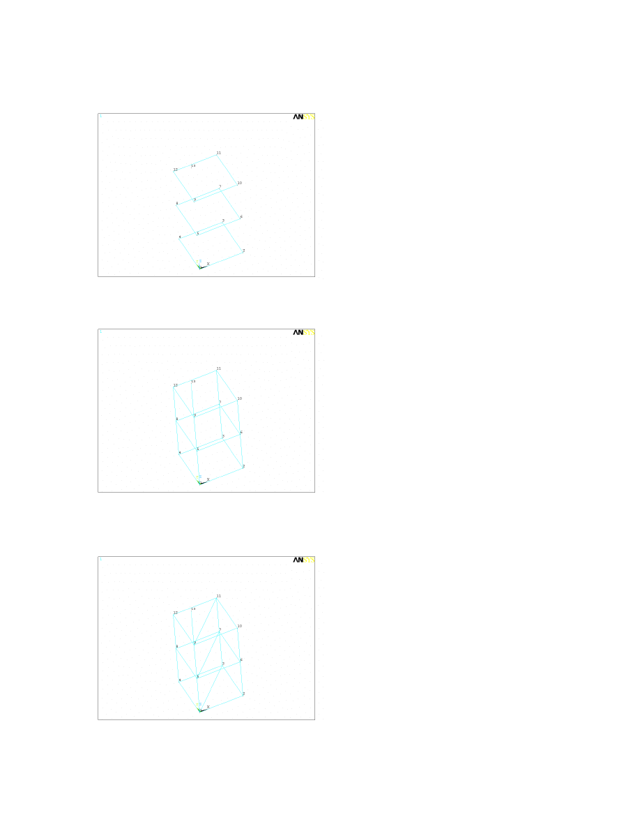
ends, then clicking ‘Apply’; create elements in a square pattern between nodes 1-2-3-4, 5-6-7-8, and 9-10-
11-12, as shown in Figure 4.2 (note that node 1 is at the origin and is not visibly numbered).

Figure 4.2

4. Now create vertical elements between vertically adjoining nodes, as shown in Figure 4.3.

Figure 4.3

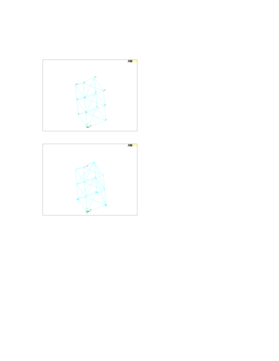
5. Now create diagonal elements across each horizontal square pattern of elements, going from the corner
nearest the origin to the corner opposite, as shown in the Figure 4.4.

Figure 4.4

Page

19

6. Finally, create the out-of-plane diagonal elements. These should slope down from the node in one tier
closest to the origin to the adjoining nodes in the one below (Figure 4.5), and from the node in one tier
farthest from the origin to those same nodes in the one below. There should also be one last element from
node 13 to node 11. The final configuration should match Figure 4.1 (repeated below).

Figure 4.5

Figure 4.1 (repeated)

Solution

Next we will apply loads and support displacements, then solve the problem.

Applying displacements:

1. On the Solution menu, under the ‘-Loads-‘ heading click ‘Apply’.

2. Click ‘Displacement’.

3. Click ‘On Nodes’.

4. Pick nodes 1, 2, 3, and 4, then click ‘OK’.

5. Select ‘All DOF’ and enter a displacement value of 0. This fixes the nodes at the bottom of the truss.

Applying loads:

1. On the Apply menu, click ‘Force/Moment’.

Page

20

2. Click ‘On Nodes’.

3. Click node 13, then click ‘OK’.

4. Leave the direction of the force as ‘FX’, and enter a value of 1000, then click ‘OK’.

Solving the problem:

1. Under the ‘-Solve-‘ heading of the Solution menu, click ‘Current LS’. Review the information presented,
and if everything seems in order, click ‘OK’. ANSYS will solve the problem.

Postprocessor

Finally we will view the deformed shape and list the member forces in the Postprocessor.

Viewing the deformed shape:

1. On the General Postprocessor menu, click ‘Plot Results’.

2. Click ‘Deformed Shape’.

3. Choose ‘Def + undef edge’ to see the deformed shape plus the edges of the original shape, then click
‘OK’.

Listing member forces:

1. On the General Postprocessor menu, click ‘List Results’.

2. Click ‘Element Solution’.

3. Click ‘Nodal force data’ in the left window, then click ‘OK’. A listing of the forces in each element will
appear.

Example 5: Simple 2-D Heat Transfer

In this example we will solve a simple transfer problem on the plate-with-three-holes model we used for
our first example on static 2-D stress analysis.

Preprocessor

First we will read in the database file from the original example.

Reading in the database:

1. On the ‘File’ menu on the menu bar at the top of the screen, click ‘Resume from’.

2. In the file selection box that appears, find and select your database file, then click ‘OK’.

Next we will define the new element type.

Defining an element type:

1. On the Preprocessor menu, click ‘Element Type’.

Page

21

2. Click ‘Add/Edit/Delete’.

3. Click ‘Add’

4. Choose ‘Solid’ under the Thermal heading in the left box (you will need to scroll down), and ‘Quad
4node 55’ in the right box, then click ‘OK’. This selects a four-noded quadrilateral 2-D thermal element.

Next we will input the additional material property needed for this thermal problem: The material’s thermal
conductivity.

Defining material properties:

1. Click ‘Material Props’ on the Preprocessor menu.

2. Click ‘Material Models’, then click ‘OK’.

3. Double-click ‘Thermal’ in the right side of the window, then ‘Conductivity’, then ‘Isotropic’.

4. Enter 154 in the box marked ‘KXX’ (154 W/m-K is the thermal conductivity of 6061-T4 aluminum),
then click ‘OK’.

Now we will destroy the old mesh and create a new one using the new thermal element type.

Meshing:

1. On the Preprocessor menu, click ‘MeshTool’.

2. Click ‘Clear’ (near the bottom of the box).

3. Click on the plate, then click ‘OK’ in the Clear Areas pick box (or just click ‘Pick All’ in the pick box).
The elements will now be removed (all if you have plotted the elements, they will still be shown in the
graphics window).

4. Now, in the Element Attributes section of the MeshTool, choose ‘Global’ and click ‘Set’.

5. Click on the box labeled ‘Element type number’, then select the PLANE55 element (the thermal element
defined earlier). Now click ‘OK’.

6. Click ‘Mesh’, then ‘Pick All’ in the Mesh pick box. ANSYS will now mesh the model with thermal four-
noded quadrilateral elements.

7. Close the MeshTool.

Solution

Next we apply thermal “loads” and solve the problem in the Solution phase. First we will remove the old
displacement and load boundary conditions from the earlier analysis.

Applying loads:

1. Click ‘Delete’ under the ‘-Loads-‘ heading on the Solution menu.

2. Click ‘All Load Data’.

3. Click ‘All Loads & Opts’.

4. Click ‘OK’ in the confirmation box.

Page

22

Now we will apply the thermal boundary conditions.

Applying boundary conditions:

1. Click ‘Apply’ under the ‘-Loads-‘ heading on the Solution menu.

2. Under the ‘-Thermal-‘ heading, click ‘Temperature’.

3. Click ‘On lines’.

4. Pick the left edge of the plate, then click ‘OK’ in the pick box.

5. Enter 0 into the box for load TEMP value (for 0 degrees Celsius, or whatever reference temperature you
choose), then click ‘OK’.

6. Now click ‘Heat Flux’ under the ‘-Thermal-‘ heading on the Apply menu.

7. Click ‘On Lines’.

8. Click the right edge of the plate, then click ‘OK’ in the pick box.

9. Enter a heat flux of 100 (100 W/m per meter depth of the plate), then click ‘OK’.

The other sides are left “free”, which corresponds to perfectly insulated conditions (zero heat flux).

Now we have finished applying boundary conditions and are ready to solve the problem. Click ‘Current
LS’ under the ‘-Solve-‘ heading on the solution menu (as usual).

Postprocessor

Finally, we will display the results in the Postprocessor.

1. On the Postprocessor menu, click ‘Plot Results’.

2. Click ‘Nodal Solu’.

3. Choose ‘DOF solution’ in the left box, and ‘Temperature’ in the right (you will have to scroll down),
then click ‘OK’.

A plot of the temperature distribution will appear (not shown, as it has few unusual features).

Example 6: Modal Analysis

In this example we will find the first five natural modes and frequencies of a square plate with simply
supported edges and a circular hole at its center, shown in Figure 6.1.

Page

23

Figure 6.1

Preprocessor

Element type:

Since this is an essentially three-dimensional problem (because of the out-of-plane vibration modes of the
plate), we will need a shell element rather than a simple 2-D quadrilateral.

1. On the Preprocessor menu, click ‘Element Type’.

2. Click ‘Add/Edit/Delete’.

3. Click ‘Add’.

4. Choose ‘Shell’ under the Structural heading from the list on the left, and ‘Elastic 8node 93’ from the list
on the right, then click ‘OK’.

Real constants:

The plate thickness is necessary to solve this problem, and is input as a real constant.

1. Click ‘Real Constants’ on the Preprocessor menu.

2. Click ‘Add’.

3. Click ‘OK’ in the Element Type for Real Constants box (there is only the one element type to define real
constants for).

4. Enter 0.001 (1 mm) in all four boxes for shell thickness, then click ‘OK’. (It is possible to define
different thicknesses for different nodes on the plate, but we will choose a plate of uniform thickness here.)

Material properties:

We will use generic values for aluminum for this problem.

1. Click ‘Material Props’ on the Preprocessor menu.

Page

24

2. Click ‘Material Models’, then click ‘OK’.

3. Double-click ‘Structural’ in the right side of the window, then ‘Linear’, then ‘Elastic’, then finally
‘Isotropic’.

4. Enter in 70e9 (70 GPa) for Young’s modulus, and 0.3 for Poisson’s ratio, then click ‘OK’.

5. Double-click ‘Density’ in the right side of the window, then enter 2.7e3 (2700 kg/cubic meter) for the
material’s density and click ‘OK’.

Modeling:

Now we will create the model.

1. Under the ‘-Modeling-‘ heading on the Preprocessor menu, click ‘Create’.

2. Under the ‘-Areas-‘ heading, click ‘Rectangle’.

3. Click ‘By Dimensions’.

4. Enter in the following values:

X1,X2

-0.5

0.5

Y1,Y2

-0.5

0.5

This creates a square 1 meter on a side, centered at the origin.

5. Now click ‘Circle’ under the ‘-Areas-‘ heading on the Create menu.

6. Click ‘By Dimensions’.

7. Enter 0.2 for the outer radius, then click ‘OK’.

8. Now close the Circle and Create menus, and under the ‘-Modeling-‘ heading on the Preprocessor menu,
click ‘Operate’.

9. Under the ‘-Booleans-‘ heading, click ‘Subtract’.

10. Click ‘Areas’.

11. Click on the square, then click ‘OK’ to select the square to be subtracted from. (A box will appear
saying that there are 2 areas at the selected location, and that area 1 is selected. Area 1 will be the square, so
just click ‘OK’.)

12. Next, click on the circle, then click ‘OK’ to subtract the circle from the square. (The same box as
previously will appear; this time click ‘Next’ to designate area 2 -- the circle—to be subtracted, then click
‘OK’.)

You have now finished constructing your model.

Meshing:

1. On the Preprocessor menu, click ‘MeshTool’.

2. Under Lines in the Size Controls section, click ‘Set’.

3. In the pick box, click ‘Pick All’.

Page

25

4. Enter 10 into the box for number of element divisions, then click ‘OK’.

5. In the MeshTool box, click ‘Mesh’; in the pick box that appears, click ‘Pick All’. ANSYS will now mesh
the model.

You are now done with the Preprocessor.

Solution

Defining the analysis:

1. On the Solution menu, click ‘New Analysis’.

2. Choose ‘Modal’, then click ‘OK’.

3. On the Solution menu, click ‘Analysis Options’.

4. Enter 5 in the box for number of modes to extract and set the mode extraction method to ‘Subspace’,
then click ‘OK’. Since we have defined a fairly fine mesh, we can easily get accurate results for this many
modes.

5. Click ‘OK’ in the box for subspace modal analysis options.

Applying boundary conditions:

1. On the Solution menu under the ‘-Loads-‘ heading, click ‘Apply’.

2. Click ‘Displacement’.

3. Click ‘On Lines’.

4. Click the top and bottom of the plate, then click ‘OK’. (Both the top and bottom will have the same
degrees of freedom constrained.)

5. Select ‘UY’ to be constrained, then enter a displacement value of 0 and click ‘Apply’.

6. Select the left and right sides of the plate, then click ‘OK’.

7. Select ‘UX’ to be constrained, then enter a displacement value of 0 and click ‘Apply’.

8. Finally, since all the edges need to be constrained in the Z direction, click all four edges of the plate, then
click ‘OK’.

9. Select ‘UZ’ to be constrained, then enter a displacement value of 0 and click ‘OK’.

Solving the problem:

1. On the Solution menu under the ‘-Solve-‘ heading, click ‘Current LS’.

2. Review the analysis summary information presented; in particular, make sure that the number of modes
to extract is the number that you want. If everything is in order, click ‘OK’ in the Solve Current Load Step
window. ANSYS will now solve the problem. (For modal analysis, ANSYS may give a warning that the
mode shapes found will be for viewing purposes only; you can ignore this.)

You are now done with the Solution phase.

Page

26

Postprocessor

Viewing the mode shapes:

1. On the General Postprocessor menu under the ‘-Read Results-‘ heading, click ‘First Set’.

2. Click ‘Plot Results’.

3. Under the ‘-Contour Plot-‘ heading, click ‘Nodal Solu’.

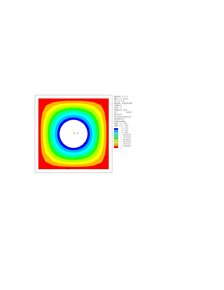
4. Choose ‘DOF solution’ in the box on the left, and ‘Translation UZ’ in the right to see the out-of-plane
displacements. The mode frequency will be displayed on the right side of the graphics window as ‘FREQ’.

5. To view the other modes, go back to the General Postprocessor menu, click ‘Next Set’ under the ‘-Read
Results-‘ heading, then repeat steps 2-4 above. The first mode is shown in Figure 6.2

Figure 6.2

Example 7: Plate Buckling Analysis Part 1: Eigenvalue Buckling
Analysis

In the first part of this example we will find the critical load for buckling of a thin flat plate by eigenvalue
buckling analysis. From the ANSYS online help:

“Eigenvalue buckling analysis predicts the theoretical buckling strength of an ideal linear elastic structure.
This method corresponds to the textbook approach to elastic buckling analysis ... However, imperfections
and nonlinearities prevent most real-world structures from achieving their theoretical elastic buckling
strength.”

The second part of this example will detail the second, more accurate type of buckling analysis available in
ANSYS—nonlinear buckling analysis.

Page

27

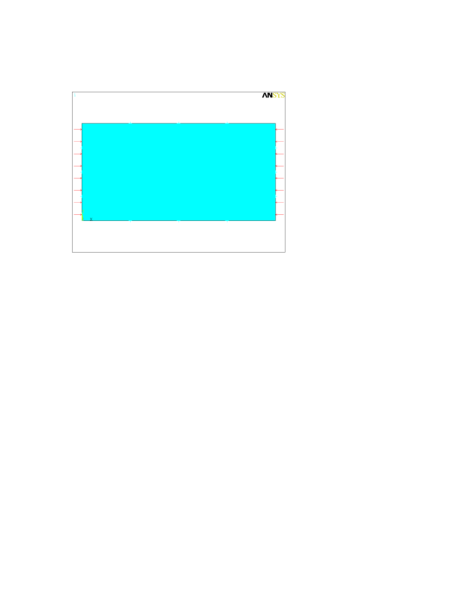
The plate to be analyzed is shown in Figure 7.1. It is 20 cm long, 10 cm wide, 1 mm thick, and made of
steel with E = 210 GPa and nu = 0.3. Thin plate buckling theory predicts that it will buckle in the second
mode when the applied load is 75.9 kN/m.

Figure 7.1

Eigenvalue buckling analysis in ANSYS has four steps:

1. Build the model

2. Obtain the static solution

3. Obtain and expand the eigenvalue buckling solution

4. Review the results

Preprocessor

Element type:

Because the plate will develop out-of-plane displacements, we will need to use a shell element type for it.

1. On the Preprocessor menu, click ‘Element Type’.

2. Click ‘Add/Edit/Delete’.

3. Click ‘Add’.

4. Choose ‘Shell’ under the Structural heading from the list on the left, and ‘Elastic 8node 93’ from the list
on the right, then click ‘OK’.

Real constants:

1. Click ‘Real Constants’ on the Preprocessor menu.

2. Click ‘Add’.

3. Click ‘OK’ in the Element Type for Real Constants box.

Page

28

4. Enter 0.001 (1 mm) in all four boxes for shell thickness, then click ‘OK’.

Material properties:

1. Click ‘Material Props’ on the Preprocessor menu.

2. Click ‘Material Models’, then click ‘OK’.

3. Double-click ‘Structural’ in the right side of the window, then ‘Linear’, then ‘Elastic’, then finally
‘Isotropic’.

4. Enter in 210e9 (210 GPa) for Young’s modulus and 0.3 for Poisson’s ratio, then click ‘OK’.

Modeling:

1. Under the ‘-Modeling-‘ heading on the Preprocessor menu, click ‘Create’.

2. Under the ‘-Areas-‘ heading, click ‘Rectangle’.

3. Click ‘By Dimensions’.

4. Enter in the following values:

X1,X2

0

0.2

Y1,Y2

0

0.1

Then click ‘OK’.

Meshing:

1. On the Preprocessor menu, click ‘MeshTool’.

2. Under Lines in the Size Controls section, click ‘Set’.

3. Pick the left and right edges of the plate, then click ‘OK’.

4. Set the number of element divisions to 8, then click ‘Apply’. (We desire a reasonably fine mesh for
accuracy, but of course not too fine.)

5. Pick the top and bottom edges of the plate, and set the number of element divisions to 16.

6. Choose ‘Map’ under the Mesher heading. This will give a simple grid of elements from the line size
controls we just set.

7. Click ‘Mesh’, then click ‘Pick All’ on the Mesh Areas pick box. (This is faster than picking the plate,
then clicking ‘OK’). ANSYS will now mesh the plate.

You are now done with the Preprocessor.

Solution (static analysis)

Applying boundary conditions:

1. Click ‘Apply’ under the ‘-Loads-‘ heading on the Solution menu.

2. Click ‘Displacement’.

Page

29

3. Click ‘On Lines’.

4. Click ‘Pick All’ in the pick box to apply displacement to all the edges.

5. Select UZ to be constrained, then enter a displacement value of 0 and click ‘OK’.

Applying loads:

The eigenvalue buckling analysis outputs scale factors on the pre-existing loads rather than loads
themselves, so it is most convenient to apply unit loads.

1. On the Apply Loads menu, click ‘Pressure’.

2. Click ‘On Lines’.

3. Pick the left and right edges of the plate, then click ‘OK’.

4. Enter in a pressure value of 1, then click ‘OK’.

Turning on prestress effects:

Prestress effects must be included in an eigenvalue buckling analysis. Turn on prestress effects by typing
“PSTRES,ON” (without the quotes) and pressing Enter in the ANSYS command window. WITHOUT
TURNING ON PRESTRESS EFFECTS YOU WILL NOT BE ABLE TO PERFORM THE BUCKLING
ANALYSIS.

Solving the static analysis:

1. On the Solution menu under the ‘Solve’ heading, click ‘Current LS’.

2. Review the solution information given. If everything is in order click ‘OK’. ANSYS will then solve the
static analysis.

Solution (eigenvalue buckling analysis)

Setting the eigenvalue buckling analysis type:

1. On the Solution menu under the ‘-Analysis Type-‘ heading, click ‘New Analysis’.

2. Choose ‘Eigen Buckling’, then click ‘OK’. The Solution menu will disappear after this, and you will
need to bring it back up.

Setting analysis options:

1. On the Solution menu, click ‘Analysis Options’.

2. Set the mode extraction method to ‘Subspace’, and enter in 2 for the number of modes to extract (we are
only interested in the first mode in which it buckles, but the absence of any constraints on rotation about the
Z axis will introduce an extra “buckling” mode of simple rotation at a load of approximately 0). Then click
‘OK’.

3. In the Subspace Eigenvalue Buckling box that appears, leave all the settings at their defaults and click
‘OK’.

Page

30

Setting mode expansion options:

1. Under the ‘-Load Step Opts-‘ heading, click ‘ExpansionPass’.

2. Click ‘Expand Modes’.

3. Enter 2 in the box for number of modes to expand, then click ‘OK’.

Solving the eigenvalue buckling analysis:

1. On the Solution menu under ‘-Solve-‘, click ‘Current LS’.

2. Review the solution information given. If everything is in order click ‘OK’. ANSYS will then solve the
eigenvalue buckling analysis.

Postprocessor

Listing buckling loads:

1. On the General Postprocessor menu, click ‘Results Summary’. The number in the ‘TIME/FREQ’ column
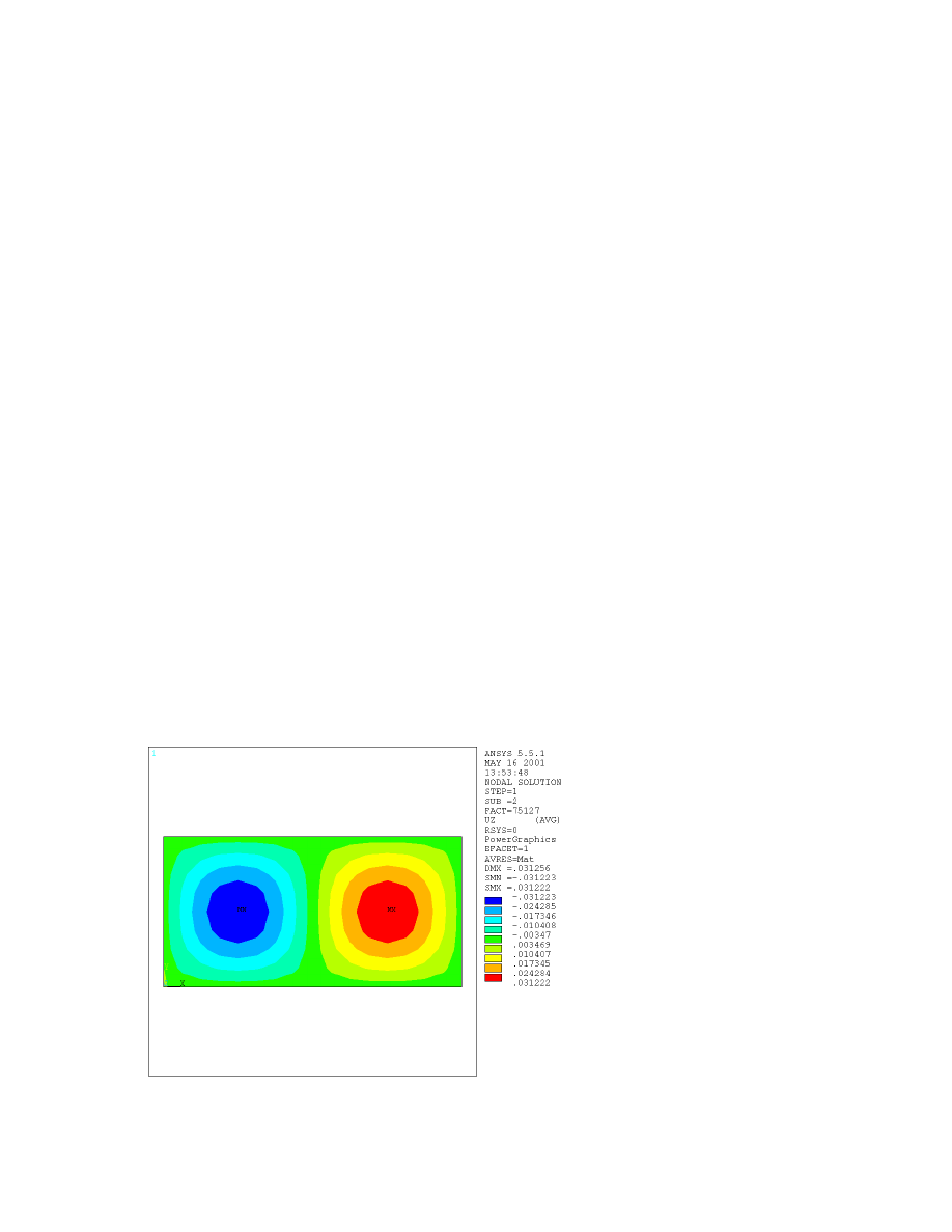
is the buckling load. ANSYS gives the buckling load as 75,127 N/m, close to the expected value of 75.9
kN/m.

Viewing the buckled shape:

1. On the General Postprocessor menu under the ‘-Read Results-‘ heading, click ‘Last Set’. This will read
in the second set of mode results, the one for the actual buckling mode.

2. On the General Postprocessor menu, click ‘Plot Results’.

3. Under the ‘-Contour Plot-‘ heading, click ‘Nodal Solu’.

4. In the left box select ‘DOF solution’, and in the right box select ‘Translation UZ’, then click ‘OK’.
Figure 7.2 shows the results; the plate buckles in mode 2 as expected.

Figure 7.2

Page

31

Example 8: Plate Buckling Analysis Part 2: Nonlinear Buckling
Analysis

In the second part of this example we will find the critical load for buckling of a thin flat plate by nonlinear
buckling analysis.

Nonlinear buckling analysis in ANSYS is somewhat simpler than eigenvalue buckling analysis since there
is only one solution step; however, it can require more than one load step in solution. In general, a
nonlinear buckling analysis is simply a nonlinear static analysis in which the load is increased until the
solution fails to converge, indicating that the structure cannot support the applied load (or that numerical
difficulties prevent solution). If the structure does not lose its ability to support additional load when it
buckles (the plate we are analyzing is an example of such a structure), a nonlinear buckling analysis can
also be used to track post-buckling behavior. We will not carry out post-buckling analysis here because of
uncertainty in the validity of the results.

We will use the plate model from the previous part of this example, so we do not need to use the
Preprocessor.

Solution

Setting the analysis type:

1. On the Solution menu, click ‘New Analysis’.

2. Choose ‘Static’, then click ‘OK’.

3. Click ‘Analysis Options’.

4. Set large deformation effects (NLGEOM) to ‘ON’.

5. Under the ‘[SSTIF][PSTRES]’ heading near the bottom of the box, click the box next to ‘Stress stiffness
or prestress’ and choose ‘Stress stiff ON’. Then click ‘OK’.

Applying loads:

We will use two load steps for this problem. From the ANSYS manual, “A load step is simply a
configuration of loads for which a solution is obtained.” Each load step is divided into one or more
substeps, where solutions are calculated. In a nonlinear static analysis, multiple substeps are used to apply
the loads gradually so that a more accurate solution can be obtained; in a dynamic analysis they are used to
specify time steps for integration. For this problem we will use one load step to load the plate edges up to
70 kN/m, then another to slowly increase the load from 70 kN/m to 80 kN/m, past the expected buckling
load. We will also apply a small out-of-plane load to the plate where maximum displacement occurred in
the eigenvalue buckling analysis, to generate the initial out-of-plane displacement to get buckling started.

First load step:

1. Under the ‘-Loads-‘ heading on the Solution menu, click ‘Apply’.

2. Click ‘Pressure’.

3. Click ‘On Lines’.

Page

32

4. Pick the left and right edges of the plate, then click ‘OK’.

5. Enter a pressure value of 70e3, then click ‘OK’.

6. On the Apply Loads menu, click ‘Force/Moment’.

7. Click ‘On Nodes’.

8. Click the fourth node from on the left on the centerline of the plate, then click ‘OK’.

9. Select ‘FZ’ for the force direction and enter a load value of 0.1 (0.1 N), then click ‘OK’. This is the load
to generate the out-of-plane displacements

10. Under the ‘-Load Step Opts-‘ heading on the Solution menu, click ‘Time/Frequenc’.

11. Click ‘Time and Substeps’.

12. Enter a time at end of load step of 70e3 and a number of substeps of 3. (Since this is not a time-
dependent problem, time is just a dummy variable and will be used in this case to keep track of the applied
load. The number of substeps is chosen to give the solution plenty of chance to converge.) Leave the
boundary conditions set to ‘Ramped’ to gradually apply the load.

13. On the Solution menu, click ‘Write LS File’. (You will need to click ‘Unabridged Menu’ on the
Solution menu to access this menu item in ANSYS 5.7.)

14. Enter a load step number of 1, then click ‘OK’.

Second load step:

1. Under the ‘-Loads-‘ heading on the Solution menu, click ‘Apply’.

2. Click ‘Pressure’.

3. Click ‘On Lines’.

4. Pick the left and right edges of the plate, then click ‘OK’.

5. Enter a pressure value of 80e3, then click ‘OK’.

6. Under the ‘-Loads-‘ heading on the Solution menu, click ‘Delete’.

7. Click ‘Force/Moment’.

8. Click ‘On Nodes’.

9. Pick the node where we applied the out-of-plane force, then click ‘OK’.

10. Leave the force/moment to be deleted set to ‘ALL’, and click ‘OK’.

11. Under the ‘-Load Step Options-‘ heading on the Solution menu, click ‘Output Ctrls’.

12. Click ‘DB/Results File’.

13. Choose a file write frequency of every substep, then click ‘OK’. (We will want to view the results at
every load value to determine the buckling load).

14. Under the ‘-Load Step Options-‘ heading on the Solution menu, click ‘Time/Frequenc’.

15. Click ‘Time and Substps’.

Page

33

16. Enter a time at the end of the load step of 80e3 and a number of substeps of 10. Also enter a minimum
number of substeps of 10 in the automatic time stepping section below, so that in case ANSYS decides to
perform automatic time stepping it will give at least as many load values as desired. Then click ‘OK’.

17. On the Solution menu, click ‘Write LS File’.

18. Enter a load step number of 2, then click ‘OK’.

Solving the problem:

1. Under the ‘-Solve-‘ heading on the Solution menu, click ‘From LS Files’.

2. Enter a starting LS file number of 1 and an ending file number of 2, then click ‘OK’. ANSYS will now
solve the problem. Since there are 13 total solutions specified and each is somewhat long, the solution will
take a while.

General Postprocessor

1. Under the ‘-Read Results-‘ heading on the General Postprocessor menu, click ‘First Set’.

2. Click ‘Plot Results’.

3. Under the ‘-Contour Plot-‘ heading, click ‘Nodal Solu’.

4. Choose ‘DOF solution’ in the left box and ‘Translation UZ’ in the right, then click ‘OK’. As before, the
lack of rotation constraints will mean some of the solutions will show rotation of the plate. This can be
ignored.

5. To see the rest of the results, under the ‘-Read Results-‘ heading on the General Postprocessor menu,
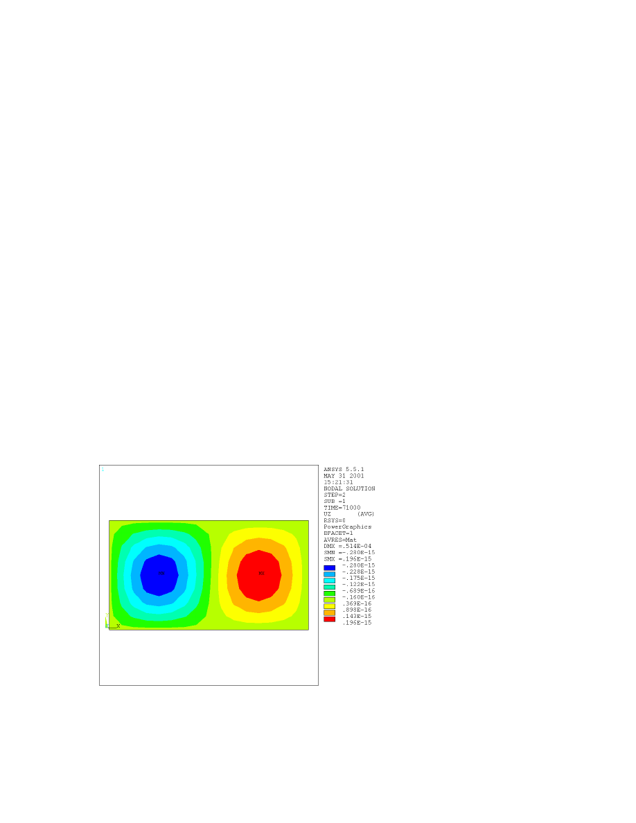
click ‘Next Set’, then repeat steps 2-4 above. From the contour plots of UZ, the plate appears to buckle at a
load between 70 kN/m and 71 kN/m (time—load—is shown at the right side of the window). The plot at 71
kN/m is shown in Figure 8.1.

Figure 8.1

This is a comparatively coarse way of determining buckling load. To get a more precise value we could
modify load step 2 to go from 70 kN/m to 71 kN/m with as many substeps as before. If the plate had

Page

34

buckled catastrophically (losing its ability to support further load), we could also have found the buckling
load quickly by activating automatic time stepping, which would have bisected the load range repeatedly
until it reached the (user-specified) minimum load increment between the upper and lower bounds on the
buckling load. However, since the plate continues to support additional load after it buckles, ANSYS
cannot tell by itself when buckling occurs in this case.

Time History Postprocessor

We will use the Time History Postprocessor to plot the out-of-plane displacement of the plate versus load.

1. On the ANSYS Main menu, click ‘TimeHist Postpro’.

2. We will need to see the elements and nodes, so click ‘Elements’ under the ‘Plot’ menu on the ANSYS
utility menu bar at the top of the screen.

3. On the TimeHist Postprocessor menu, click ‘Define Variables’.

4. Click ‘Add’.

5. Leave the variable type set to ‘Nodal DOF result’, and click ‘OK’.

6. Pick the fourth node from the right on the centerline of the plate, then click ‘OK’.

7. Choose ‘Translation UZ’ in the lower right box for the data item to be placed in a variable. You can also
define a name (such as “zdisp”) for the variable for convenience. When you are done click ‘OK’.

8. On the TimeHist Postprocessor menu, click ‘Graph Variables’.

9. Enter 2 as the first variable to graph (variables here must be referred to by their reference number rather
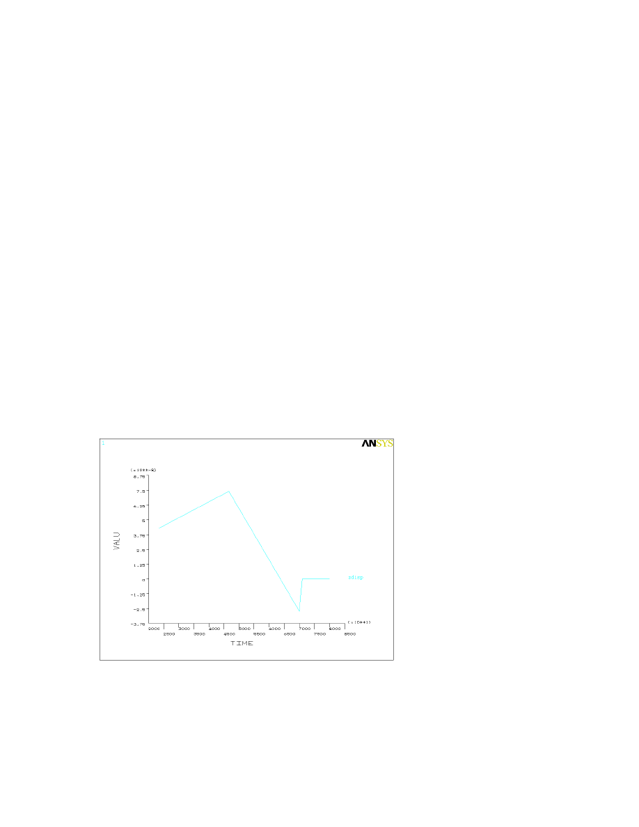
than their user-defined names), then click ‘OK’. The resulting plot is shown in Figure 8.2.

Figure 8.2

The Z displacement before 70 kN/m load is due to the out-of-plane force. The jump in z displacement from
70 kN/m to 71 kN/m corresponds to buckling, although it is less noticeable than the out-of-plane
displacements before it.

Page

35

Example 9: Simple Dynamic Analysis

In this example we will observe the deflection over time of the end of a beam hit with a short-duration
impact. The beam is 1 meter long, has a 2 cm by 2 cm square cross-section, and is made of aluminum.

Preprocessor

Element type:

1. On the Preprocessor menu, click ‘Element type’.

2. Click ‘Add/Edit/Delete’.

3. Click ‘Add’.

4. Choose ‘Beam’ under the Structural heading from the list on the left, and ‘2D elastic 3’ from the list on
the right, then click ‘OK’.

Real constants:

1. Click ‘Real constants’ on the Preprocessor menu.

2. Click ‘Add’

3. Click ‘OK’ in the Element Type for Real Constants box.

4. Enter 4e-4 for the cross-sectional area, 16e-8/12 for the area moment for inertia (ANSYS will do the
arithmetic for us), and 2e-2 for the total beam height, then click ‘OK’.

Material properties:

1. Click ‘Material Props’ on the Preprocessor menu.

2. Click ‘Material Models’, then click ‘OK’.

3. Double-click ‘Structural’ in the right side of the window, then ‘Linear’, then ‘Elastic’, then finally
‘Isotropic’.

4. Enter in 70e9 for Young’s modulus, 2.7e3 for density, and 0.3 for Poisson’s ratio.

Modeling:

1. Under the ‘-Modeling-‘ heading on the Preprocessor menu, click ‘Create’.

2. Click ‘Keypoints’.

3. Click ‘In Active CS’.

4. Define the following keypoints:

Keypoint

X

Y

1

0

0

2

1

0

Page

36

5. On the Create menu, under the ‘-Lines-‘ heading click ‘Lines’.

6. Click ‘In Active Coord’.

7. Click the two keypoints, then click ‘OK’.

Meshing:

1. On the Preprocessor menu, click ‘MeshTool’.

2. Under Lines in the Size Controls section, click ‘Set’.

3. In the pick box, click ‘Pick All’. (This is faster than clicking the one line then clicking ‘OK’).

4. Enter 20 into the box for number of element divisions, then click ‘OK’.

5. In the MeshTool box, click ‘Mesh’; in the pick box, click ‘Pick All’.

The model is now meshed, and you are done in the Preprocessor.

Solution

Defining the analysis:

1. On the Solution menu, click ‘New Analysis’.

2. Choose ‘Transient’, then click ‘OK’.

Applying loads:

In a transient analysis in ANSYS, the total time span of the analysis is broken up into “load steps”, specific
periods of different loading configurations. In this analysis we will use four load steps:

x

Ramped application of the force to the end of the beam from time 0 to 10-5 seconds.

x

Constant force on the beam from 10-5 seconds to 5x10-5 seconds

x

Ramped removal of the force from 5x10-5 seconds to 6x10-5 seconds

x

No applied loads from 6x10-5 seconds to 0.06 seconds.

In defining these load steps we will take advantage of ANSYS’s feature of automatically ramping loads to
their final values.

First load step:

1. Under the ‘-Loads-‘ heading on the Solution menu, click ‘Apply’.

2. Click ‘Displacement’.

3. Click ‘On Keypoints’.

4. Click the left end of the beam, then click ‘OK’.

5. Click ‘All DOF’, then click ‘OK’.

6. On the Apply Loads menu, click ‘Force/Moment’.

7. Click ‘On Keypoints’.

8. Click the right end of the beam, then click ‘OK’.

Page

37

9. Choose the direction of the force as FY and enter a value of 1e3 (1 kN), then click ‘OK’.

10. On the Solution menu, under the ‘-Load Step Opts-‘ heading click ‘Output Ctrls’.

11. Click ‘DB/Results File’.

12. Choose a file write frequency of once every substep, then click ‘OK’.

13. On the Solution menu, under the ‘-Load Step Opts-‘ heading click ‘Time/Frequency’.

14. Click ‘Time - Time Step’.

15. Enter a time at the end of the load step of 1e-5 and a time step of 1e-6, then click ‘OK’.

16. On the Solution menu, click ‘Write LS File’. (You will need to click ‘Unabridged Menu’ on the
Solution menu to access this menu item in ANSYS 5.7.)

17. Enter a load step number of 1, then click ‘OK’.

Second load step:

We will be able to keep most of the same settings from the previous load step now.

1. On the Solution menu, under the ‘-Load Step Opts-‘ heading click ‘Time/Frequency’.

2. Click ‘Time - Time Step’.

3. Enter a time at the end of the load step of 5e-5 and a time step size of 5e-6, the click ‘OK’.

We will keep the same loading, constraints, and so forth. The force on the end of the beam was ramped in
the last load step, but since in this load step it has the same starting and ending value it will be constant.

4. On the Solution menu, click ‘Write LS File’.

5. Enter a load step number of 2, then click ‘OK’.

Third load step:

1. On the Solution menu, under the ‘-Loads-‘ heading click ‘Delete’.

2. Click ‘Force/Moment’ under the ‘-Structural-‘ heading.

3. Click ‘On Keypoints’.

4. Click the right end of the beam, then click ‘OK’.

5. Leave the force/moment to be deleted set to ‘ALL’, and click ‘OK’.

6. On the Solution menu, under the ‘-Load Step Opts-‘ heading click ‘Time/Frequency.

7. Click ‘Time - Time Step’.

8. Enter a time at the end of the load step of 6e-5 and a time step size of 1e-6, then click ‘OK’.

9. On the Solution menu, click ‘Write LS File’.

10. Enter in a load step number of 3, then click ‘OK’.

Page

38

Fourth load step:

1. On the Solution menu, under the ‘-Load Step Opts-‘ heading click ‘Time/Frequency’.

2. Click ‘Time - Time Step’.

3. Enter in a time at the end of the load step of 0.06 and a time step of 6e-4. (This will result in a large
number of individual steps in solution, but since each step in this transient analysis takes a very short
amount of time the total time for solution will still be okay.)

4. On the Solution menu, click ‘Write LS File’.

5. Enter a load step number of 4, then click ‘OK’.

Solving the problem:

1. On the Solution menu, under the ‘-Solve-‘ heading click ‘From LS Files’.

2. Enter a starting load step number of 1 and an ending load step number of 4, then click ‘OK’. ANSYS
will now solve the problem according to the load step files.

Postprocessor

For problems with multiple steps, we use the Time History Postprocessor. In this problem, we will use the
Time History Postprocessor to graph the deflection of the beam tip versus time.

1. On the ANSYS main menu, click ‘TimeHist Postpro’.

2. Click ‘Define Variables’.

3. Click ‘Add’.

4. Leave the type of variable set to ‘Nodal DOF result’ and click ‘OK’.

5. Click the right end of the beam, then click ‘OK’.

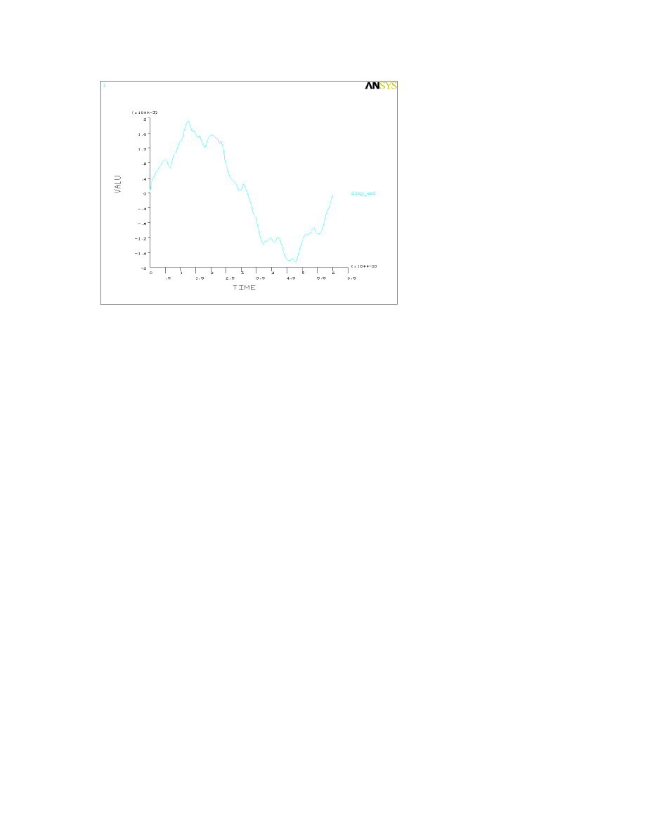
6. Choose ‘Translation UY’ from the box at the right. You can also give the variable a name such as
“disp_end” in the user-specified label box. Then click ‘OK’.

7. On the TimeHist Postprocessor menu, click ‘Graph Variables’.

8. Enter ‘2’ as the first variable to graph (in this section ANSYS only recognizes variable reference
numbers, not user-specified names). Then click ‘OK’.

The graph is shown in Figure 9.1.

Page

39

Figure 9.1

Example 10: Box Beam

In this example we will analyze a box beam—that is, a beam constructed of a thin web intended to bear
shear stress between a set of booms intended to bear normal stresses. This structure is very similar to the
idealized beam sections modeled in AA 332, except that the booms and web will be modeled as beam and
plate elements rather than axial-force-only rods and shear-only panels; this will provide a more realistic
model, and using only rods and shear panels for this sort of analysis often leaves too many unconstrained
degrees of freedom for ANSYS to solve.

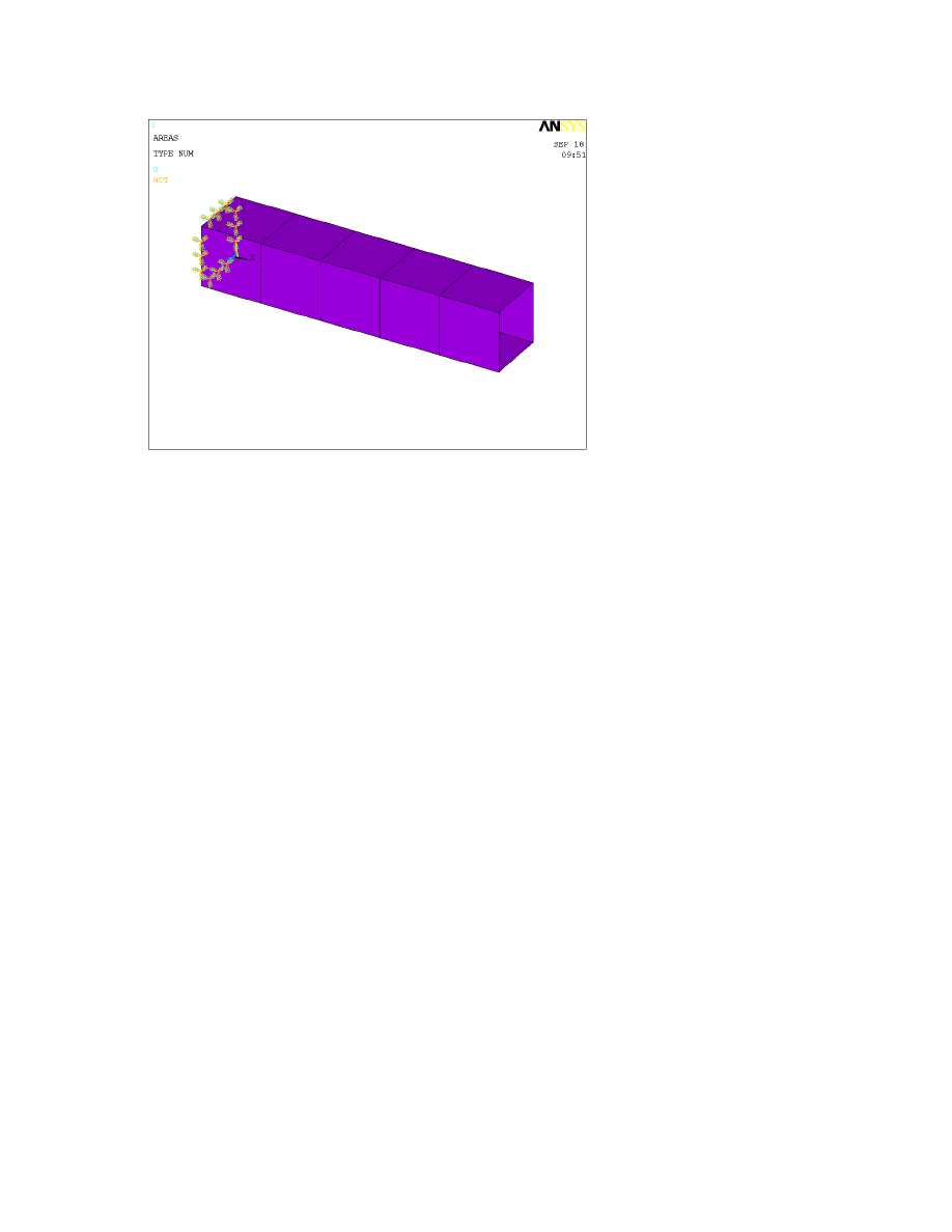
The beam to be analyzed is shown in Figure 10.1; it is 1 meter long, 20 cm wide, and 20 cm deep; the
booms have a square cross-section 1 cm on a side and the web is 0.5 mm thick. The entire structure is made
of aluminum with E = 70 GPa and nu = 0.3. A load of 1 kilonewton is applied at the center of the top boom
at the right end of the beam.

Page

40

Figure 10.1

Preprocessor

Element type:

We will need two element types for this problem: a 3D beam element and a shell element.

1. On the Preprocessor menu, click ‘Element Type’.

2. Click ‘Add/Edit/Delete’.

3. Click ‘Add’.

4. Choose ‘Beam’ under the Structural heading on the left and ‘3D elastic 4’ on the right (you will need to
scroll down), then click ‘Apply’.

5. Choose ‘Shell’ under the Structural heading on the left and ‘Elastic 4node 63’ on the right, then click
‘OK’.

Real constants:

1. Click ‘Real Constants’ on the Preprocessor menu.

2. Click ‘Add/Edit/Delete’.

3. Click ‘Add’.

3. Choose ‘Type 1 BEAM1’, then click ‘OK’.

4. Enter an area of 1e-4, second area moments of 1e-8/12, and thicknesses in the Y and Z directions of 1e-
2, then click ‘OK’.

5. Click ‘Add’ again.

6. Choose ‘Type 2 SHELL63’, then click ‘OK’.

7. Enter a thickness at each node of 0.0005, then click ‘OK’.

Page

41

Material properties:

1. Click ‘Material Props’ on the Preprocessor menu.

2. Click ‘Material Models’, then click ‘OK’.

3. Double-click ‘Structural’ in the right side of the window, then ‘Linear’, then ‘Elastic’, then finally
‘Isotropic’.

4. Enter a modulus of elasticity (“EX”) of 70e9 and a Poisson’s ratio (“PRXY”) of 0.3, then click ‘OK’.

Modeling:

Defining keypoints:

1. Under the ‘-Modeling-‘ heading on the Preprocessor menu, click ‘Create’.

2. Click ‘Keypoints’.

3. Click ‘In Active CS’.

4. Define the following keypoints, clicking ‘Apply’ after each:

Keypoint number

X

Y

Z

1

0

0

0

2

0

0.2

0

3

0

0.2

0.2

4

0

0

0.2

5

1.1

0

0

6

1.3

0

0

The last two keypoints are not part of the model; however, they will be used later to help create the areas
for the model.

When you have finished, click ‘Cancel’.

Creating lines:

1. On the ‘Create’ menu, click ‘Lines’.

2. Click ‘Straight Line’.

3. Create lines from keypoints 1-2, 2-3, 3-4, and 4-1 by clicking on the endpoints of each line. You should
have a square in the YZ plane. Note that you will need to use the Pan-Zoom-Rotate function on the
PlotCtrls menu to be able to select the points.

4. Create a line between keypoints 5 and 6, then click ‘Cancel’.

Creating areas:

1. Under the ‘-Modeling-‘ heading on the Preprocessor menu, click ‘Operate’.

2. Click ‘Extrude / Sweep’. This menu allows you to easily create prisms and bodies of revolution.

Page

42

3. Under the ‘-Lines-‘ heading, click ‘Along Lines’.

4. Select the lines in the square between keypoints 1-4, then click ‘OK’.

5. Select the line between keypoints 5 and 6, then click ‘Apply’. ANSYS will now create areas defined by
sweeping the lines selected in step 4 through the direction and length of the line just picked.

6. Repeat steps 4 and 5 (selecting the lines at the “front” of each newly created set of areas) until you have
five square tubular segments, then click ‘Cancel’. These segments will form the box beam.

7. You will now want to remove the line between keypoints 5 and 6 so that it won’t get in the way later.
Under the ‘-Modeling-‘ heading on the Preprocessor menu, click ‘Delete’.

8. Click ‘Lines and Below’. This will delete a line and all the points used to define it.

9. Click the line between keypoints 5 and 6, then click ‘OK’.

Defining element attributes:

1. On the Preprocessor menu, click ‘MeshTool’.

2. Under ‘Element Attributes’, click ‘Areas’, then click ‘Set’.

3. Click ‘Pick All’, choose real constant set 2 (for the shell elements) and element type 2 (SHELL63), then
click ‘OK’.

4. Again under ‘Element Attributes’, click ‘Lines’, then click ‘Set’.

5. Click ‘Pick All’, choose real constant set 1 (for the beam elements) and element type 1 (BEAM4), then
click ‘OK’.

Meshing:

We will use a moderate-sized mesh for this problem, since theory says that the stresses in the box beam
will not vary rapidly.

1. In the MeshTool box, under the Size Controls heading, click ‘Set’ next to ‘Global’

2. Enter 4 as the number of element divisions, then click ‘OK’.

4. Under the Mesh heading, choose ‘Areas’, then choose the mapped mesher and click ‘Mesh’.

5. Click ‘Pick All’. ANSYS will now mesh the web of the box beam.

6. Under the Mesh heading, choose ‘Lines’, then click ‘Mesh’.

7. Click ‘Pick All’. ANSYS will now mesh the booms.

You are now done with the Preprocessor.

Solution

Applying loads:

1. Under the ‘-Loads-‘ heading on the Solution menu, click ‘Apply’.

2. Click ‘Displacement’.

Page

43

3. Click ‘On Lines’.

4. Click the four lines at the back end of the box beam (in the YZ plane), then click ‘OK’.

5. Choose ‘All DOF’ as the degree of freedom to be constrained, then enter a displacement value of zero
and click ‘OK’.

6. On the ‘Apply’ menu, click ‘Force/Moment’.

7. Click ‘On Nodes’.

8. Pick the node at center of the top line at the end of the beam (the line furthest in the X and Y directions),
then click ‘OK’.

9. Choose a force direction of FY and enter a value of -1000, then click ‘OK’.

Solving the problem:

1. Under the ‘-Solve-‘ heading, click ‘Current LS’.

2. Review the information that appears. If everything appears to be in order, click ‘OK’. ANSYS will now
solve the problem.

Postprocessor

Viewing the von Mises stress in the beam:

Since aluminum is a ductile material, the von Mises failure criterion is appropriate for it. Since the von
Mises stress is a combined measure of all the stresses on a material, it will also help show whether the
stress in the sides of the beam is uniform as predicted by theory.

1. On the General Postprocessor menu, click ‘Plot Results’.

2. Under the ‘-Contour Plot-‘ heading, click ‘Nodal Solu’.

3. Choose ‘Stress’ from the left box and ‘von Mises SEQV’ from the right box (you will need to scroll
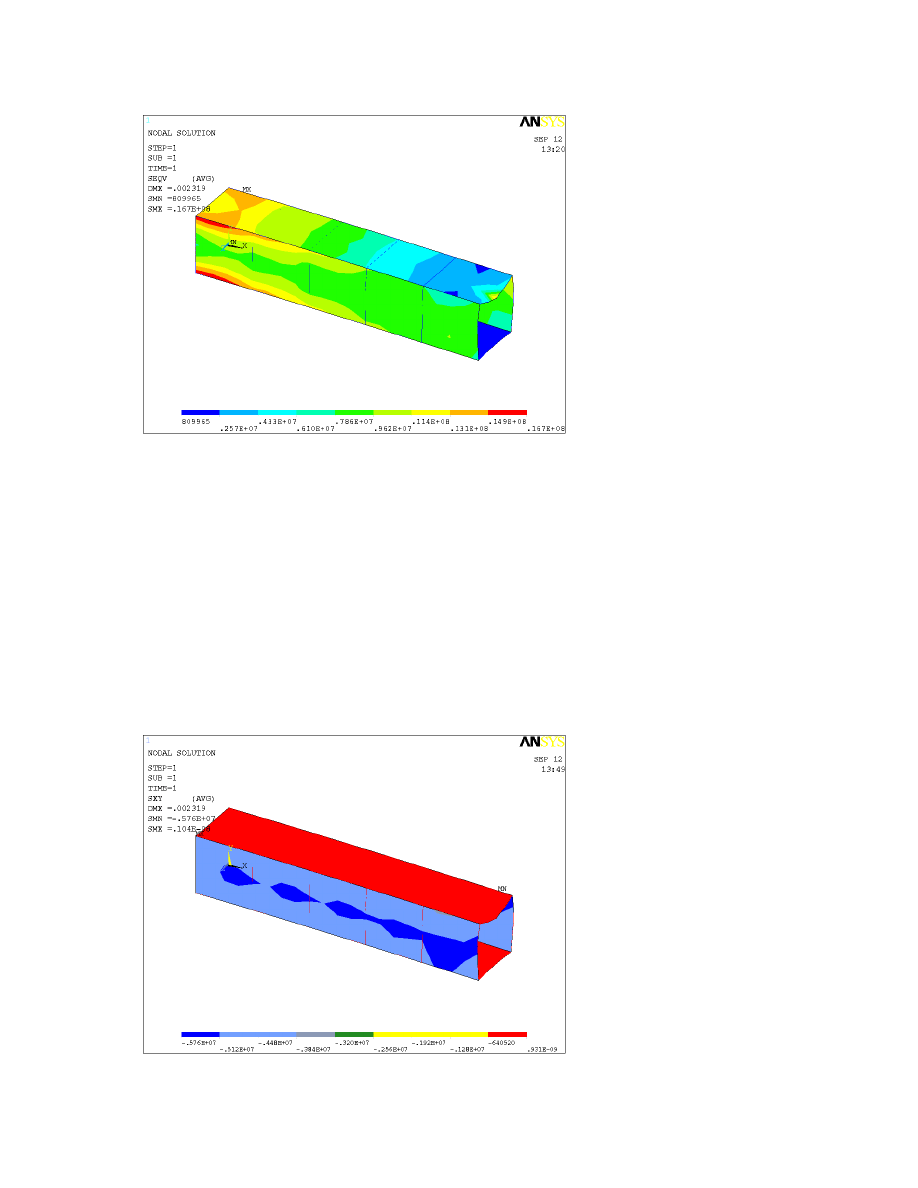
down), then click ‘OK’. A plot of the von Mises stress in the beam appears (shown in Figure 10.2).
Although the stresses are not uniform near the fixed end of the beam, further out they are close to constant.

Page

44

Figure 10.2

Viewing the shear stress in the web:

From an idealized-structure analysis, we expect the shear stress in the web at the sides to be 5 MPa and the
shear stress in the web at the top and bottom to be zero.

1. On the General Postprocessor menu, click ‘Plot Results’.

2. Under the ‘-Contour Plot-‘ heading, click ‘Nodal Solu’.

3. Choose ‘Stress from the left box and ‘XY-shear SXY’ from the right box, then click ‘OK’. The resulting
plot of shear stresses is shown in Figure 10.3; the magnitude of the stress in the side webs is close to 5
MPa, and the XY shear stress in the top and bottom webs is small. (For a more accurate estimate we could
list the results.) Plots of the other two shear stresses also yield results consistent with theory, although there
are XZ shear stress concentrations around the ends of the vertical booms.

Figure 10.3