Wykład 4: Podstawy wnioskowania

statystycznego

Biometria i

Biostatystyka

Statistical Inference

Two fundamental statistical questions
the researchers must answer repeatedly
in the course of their work:



How reliable are the results?



How probable is it that differences

between observed results and those
expected on the basis of a hypothesis
are due to chance alone?

Statistical Inference



The question of reliability is answered by

setting confidence limits to sample
statistics.



The second question involves hypothesis

testing.

Both subject belong to the field of
statistical inference.

Statistical Inference



Drawing conclusions from data



Emphasis on substantiating our

conclusions by probability calculations.



Allows us to take chance variation into account



2 most prominent types of formal

statistical inference



Confidence intervals for estimating the value of

a population parameter



Tests of significance which assess the evidence

for a claim

Statistical Inference, cont.



Inference is based on the sampling

distributions of statistics.



They report probabilities that state what would

happen if we used the inference method many

times.



When you use statistical inference you are

acting as if the data come from a random

sample or a randomized experiment.



If this is not true, your conclusions may be

open to challenge.

Distibution and variance of
mean



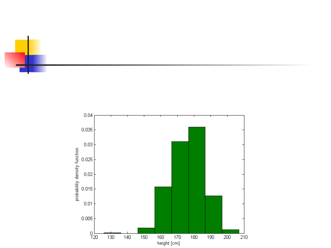
We recall our data on height.



Mean value = 176.16 cm, STD = 9.86

Distibution and variance of
mean



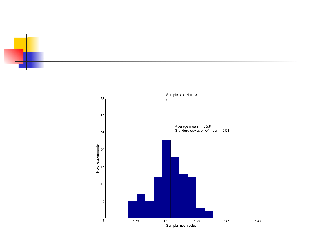
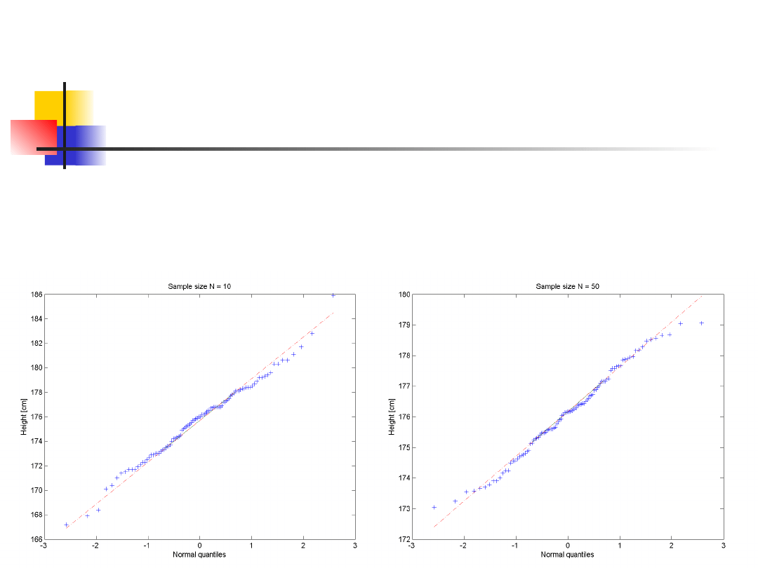
Graphs of the means of 100 samples of 10
person heights.

Distibution and variance of
mean



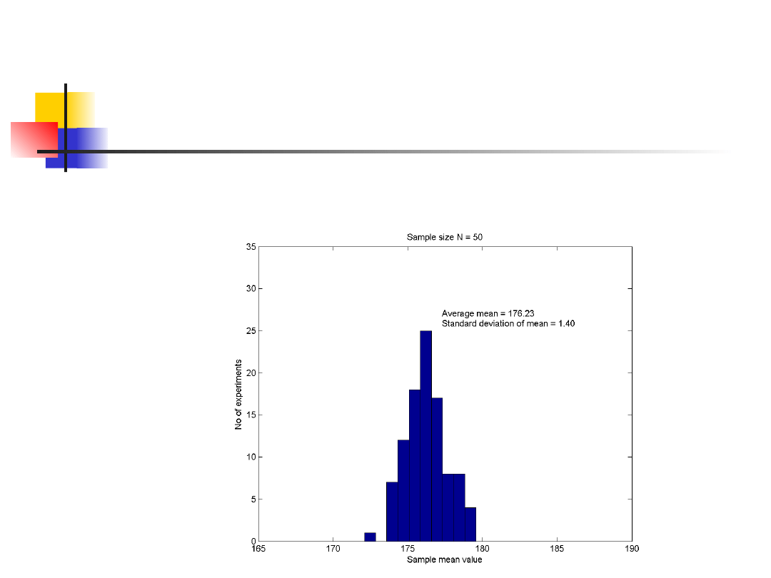
Graphs of the means of 100 samples of 50
person heights.

Distibution and variance of
mean



The means of samples from normally
distributed population are themselves
normally distributed regardless of sample
size N.

Distibution and variance of
mean



As sample size increases, the means of
samples drawn from a population of any
distribution will approach the normal
distribution.



It is known (when rigorously stated about
sampling from population with finite
variance) as the

Central Limit Theorem.

Distibution and variance of
mean

Another important fact is that

the range of the

means is considerably less than that of the
original items.



Individual height range from 126 cm to 208
cm.



The height means range from 168 cm to 183
cm in samples of 10 and from 173 cm to 179
cm in samples of 50.

Distibution and variance of
mean

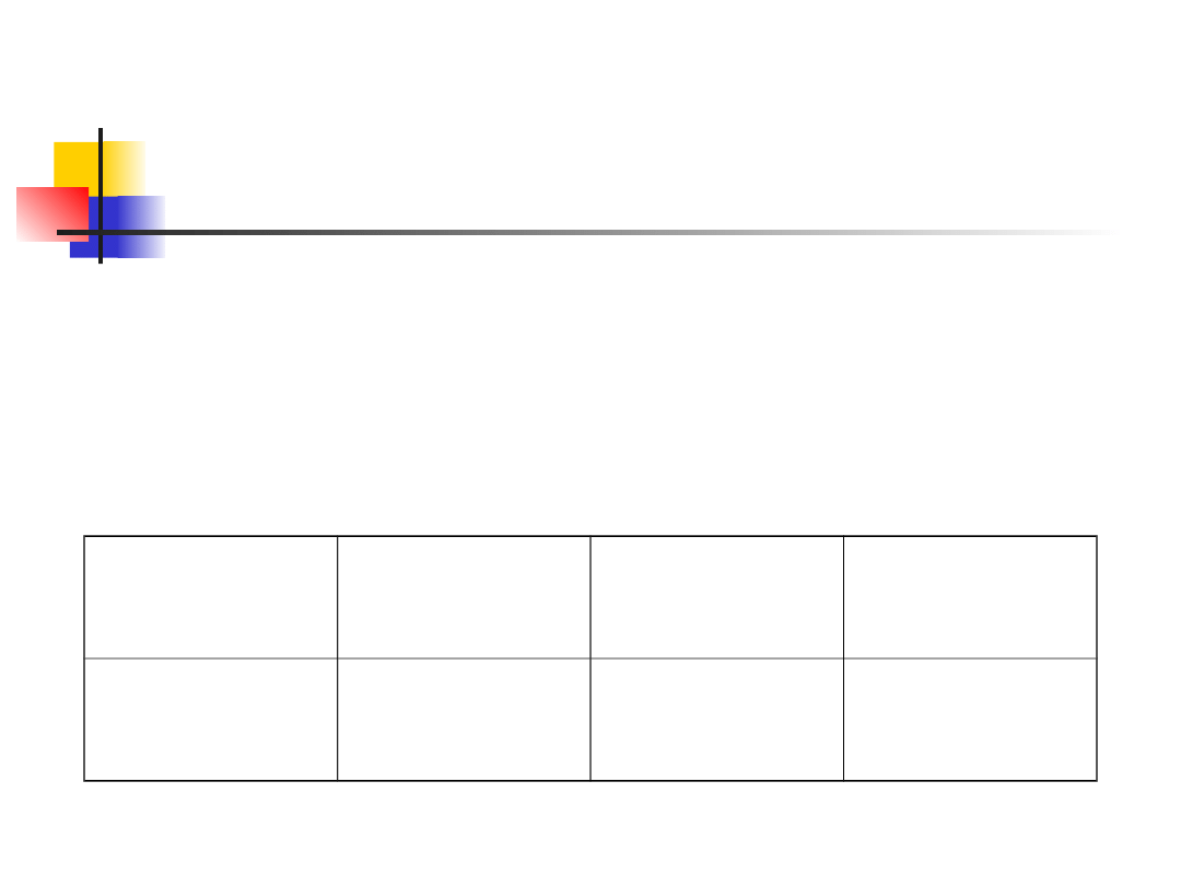
The differences in ranges are reflected

in differences in the standard
deviation of these distributions.

N=10

N=50

Populatio

n

Standard

deviation

2.94

1.40

9.86

Distibution and variance of
mean



Means based on large samples should be
close to the parametric mean and will not
vary so much as will means based on small
samples. The variance of means is therefore
partly a function of the sample size on which
the means are based.



It is also a function of the variance of the
items themselves.

Estimating with
Confidence



Draw an SRS of size n from any population
with mean



and finite standard deviation



.



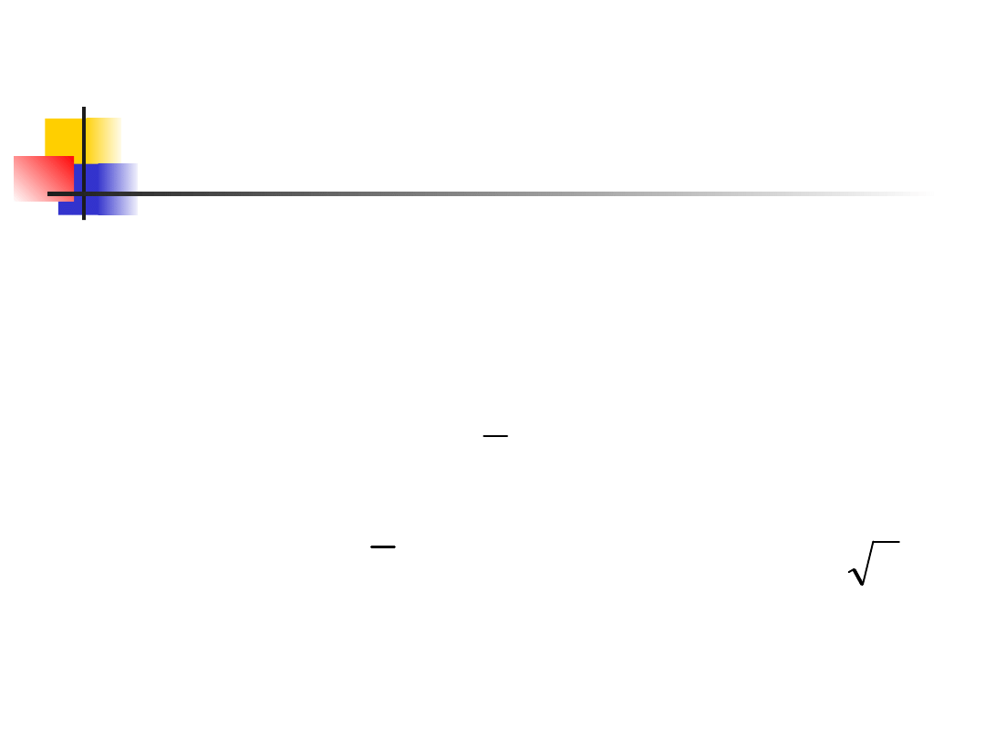
When n is large, the sampling distribution of
the sample mean is approximately normal:

is approximately

x

x





n

N

/

,





Statistical Confidence,
cont.



Let n=500, std dev = 100.



In repeated samples of size 500
the sample mean has what
distribution?



N( , 4.47) since 100/sqrt(500) =
4.47



What does the 68-95-99.7 Rule tell
me?



Statistical confidence,
cont.



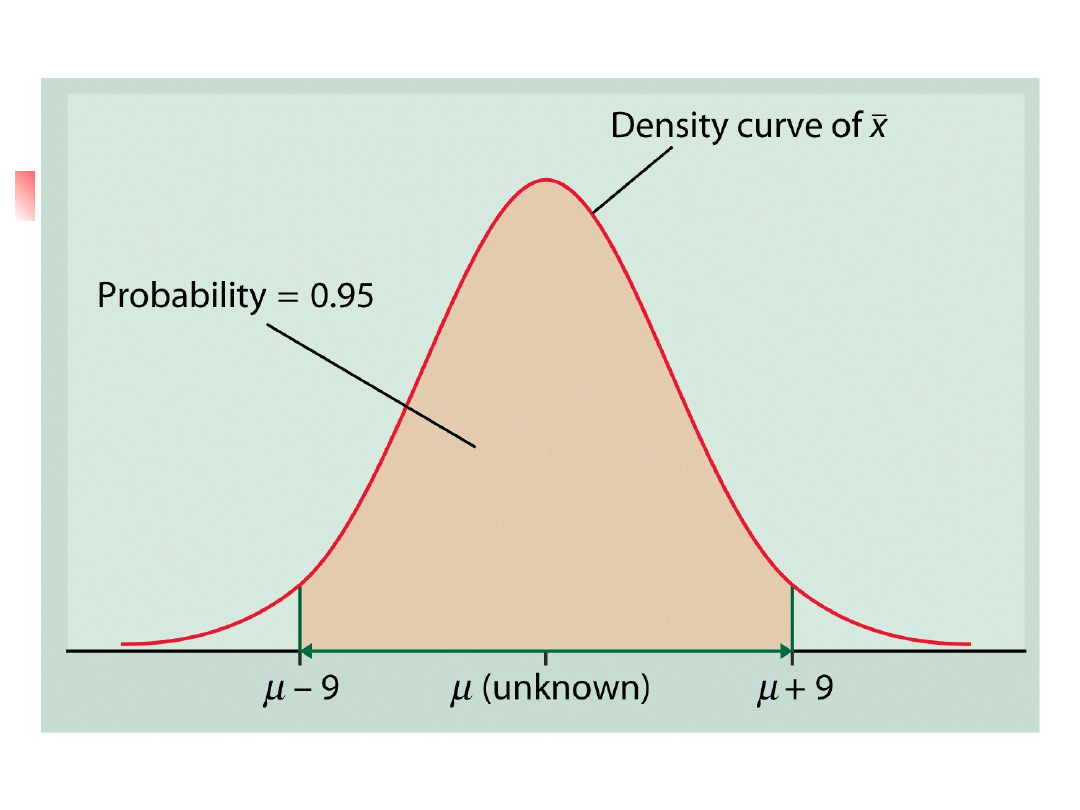
95% of all samples will capture the true
mean in the interval.



We have simply restated a fact about
the sampling distribution of



The language of statistical inference
uses this fact about what would happen
in the long run to express our
confidence in the results of any one
sample.

x

Statistical Inference, cont.



If one sample mean is equal to 461,
EITHER



The interval between 452 and 470 contains the
true mean. OR



Our SRS was one of the few samples for which
is not within 9 points of the true mean. Only
5% of all samples give such inaccurate results.



We cannot know which category our
sample falls into.

x

Confidence Intervals



The interval of numbers between the

values ( -8.94, +8.94) is called a

95% confidence interval for



Has the form (estimate – margin of

error, estimate + margin of error)



Estimate: guess for the value of the

unknown parameter



Margin of error: shows how accurate we

believe our guess is, based on the variability

of the estimate.

x

x



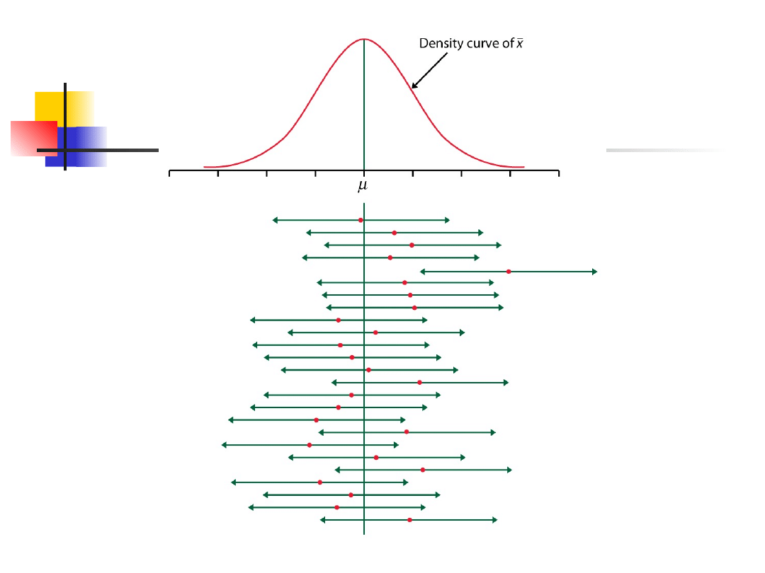
Confidence Interval



It is an interval of the form (a, b) where
a and b are number computed from the
data.



It has a property called a confidence
level that gives the probability that the
interval covers the parameter.



Most often the confidence level is 90%
or higher because we most often want
to be quite sure of our conclusions.

Confidence Interval, cont.



We will use C to stand for the confidence
level in decimal form.



95% confidence level corresponds to C=0.95



Formal definition



A level C confidence interval for a parameter
is an interval computed from sample data by
a method that has probability C of producing
an interval containing the true value of the
parameter.

Confidence interval for a
population mean



Level C confidence interval for the mean

of a population when the data are an

SRS of size n is based on the sampling

distribution of the sample mean



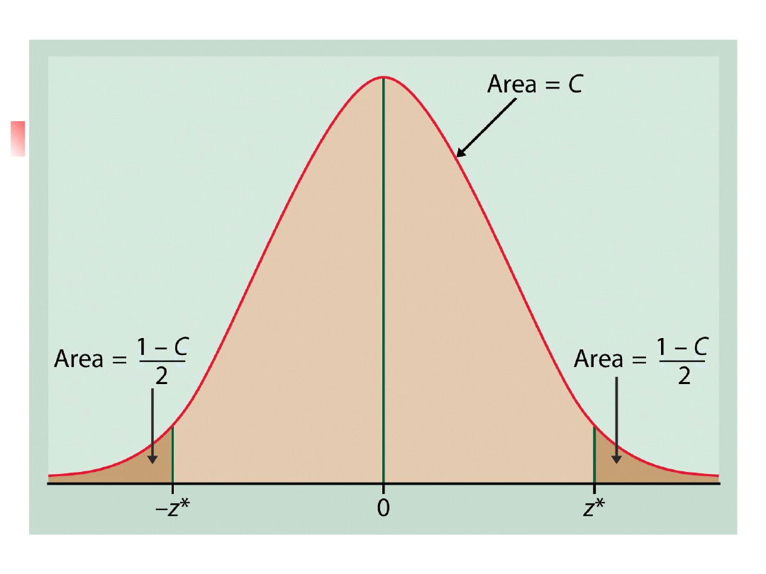
To construct a level C confidence

interval we first catch the central C area

under a normal curve.



We must find z* such that any normal

distribution has probability C within +- z*

standard deviations of its mean.



x

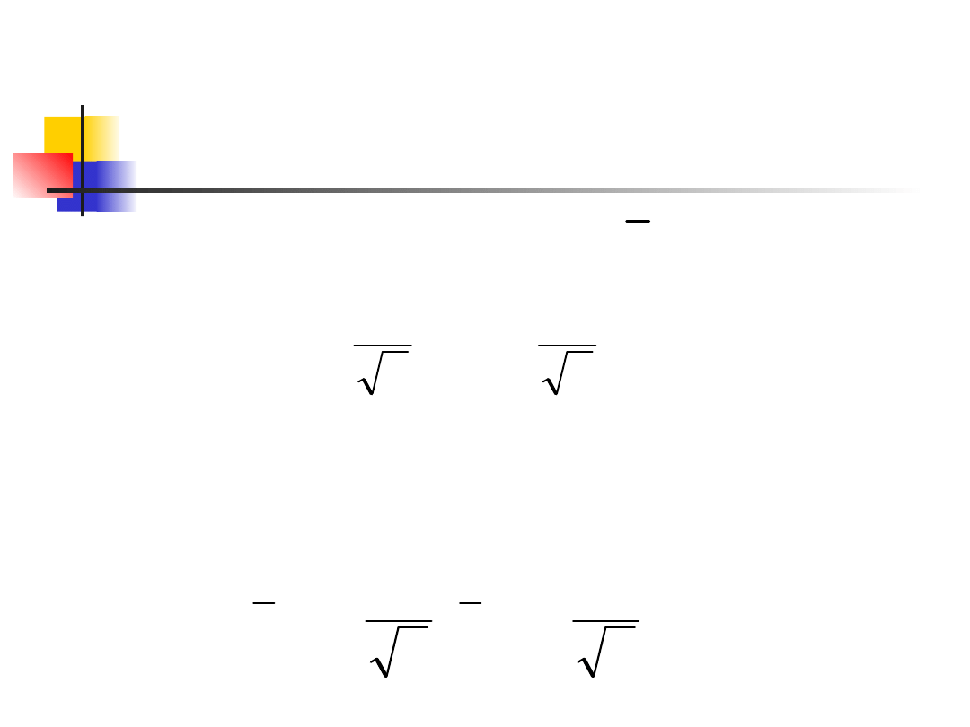
Confidence interval for a
population mean, cont.



There is probability C that lies between



This is exactly the same as saying that the
unknown population mean lies between

x

n

z

n

z









*

*

, 





n

z

x

n

z

x





*

*

, 



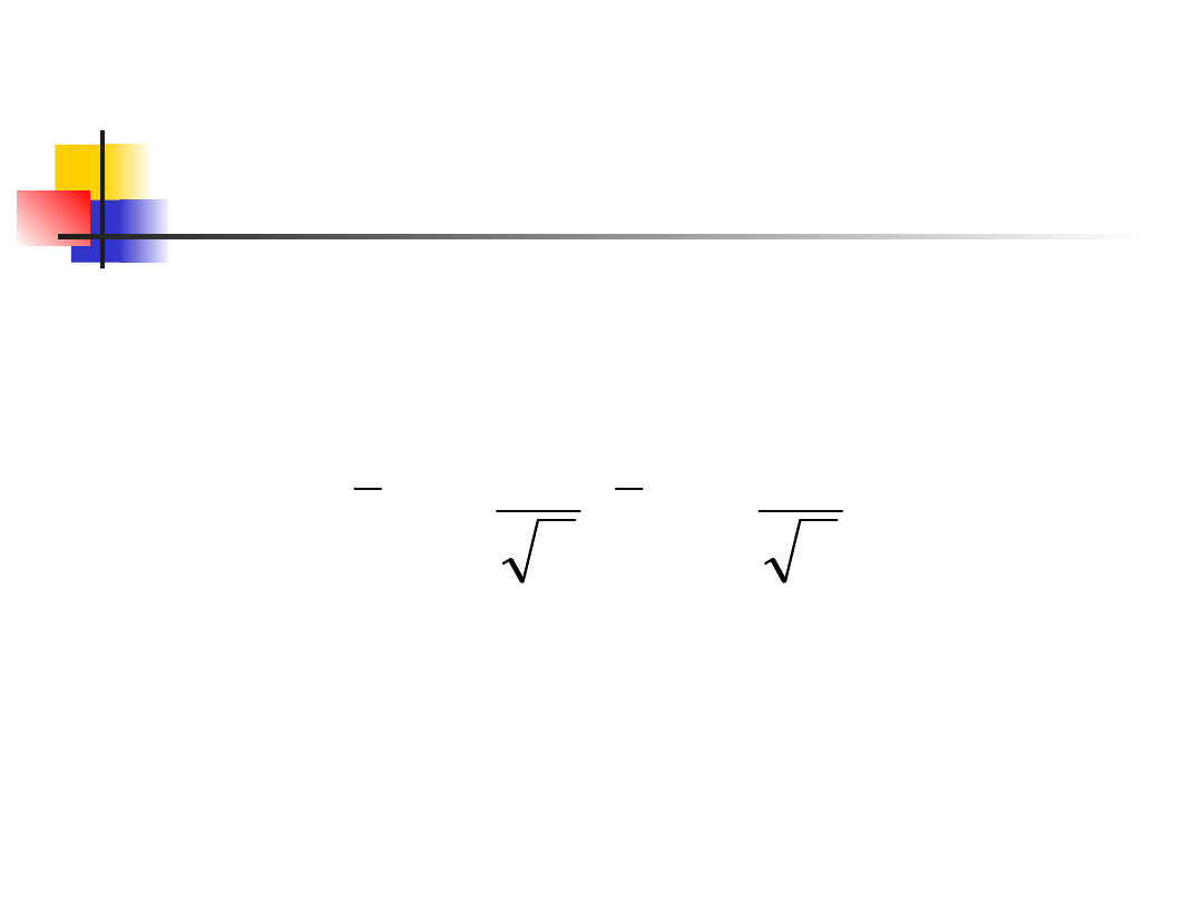
Confidence interval for a
population mean, cont.



Choose an SRS of size n from a population

having unknown mean and known standard

deviation. A level C confidence interval for

is



This interval is exact when the population

distribution is normal and is approximately

correct for large n in other cases.



n

z

x

n

z

x





*

*

, 



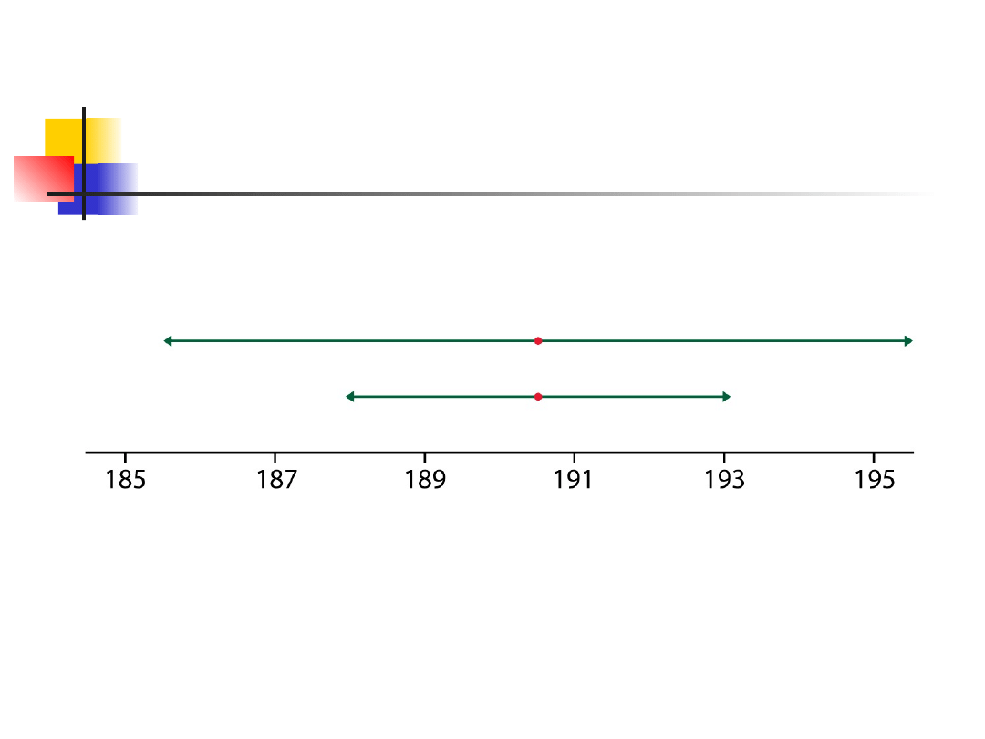
less sample size gives wider confidence

interval

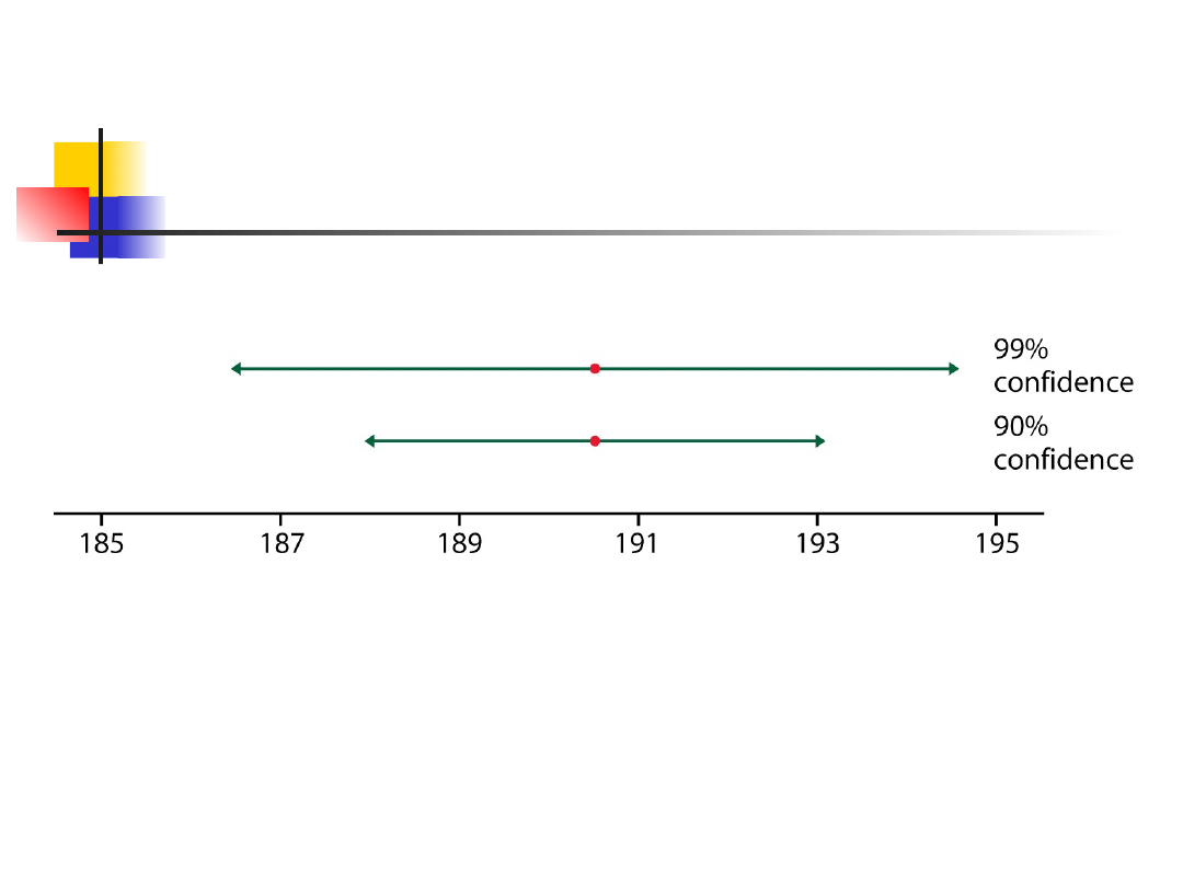
higher confidence results in wider interval

How confidence intervals
behave



Margin of error



Illustrates several important
properties that are shared by all
confidence intervals in common use.



The user chooses the confidence level,
and the margin of error follows from this
choice.

n

z



*

If your margin of error is too large…



Use a lower level of confidence (smaller C)



90% corresponds to z*=1.645



95% corresponds to z*=1.96



99% corresponds to z*=2.576



Increase the sample size (larger n)



We must multiply the number of observations by 4

in order to cut the margin of error in half.



Reduce σ.



We can sometimes reduce σ by carefully controlling

the measurement process or by restricting our

attention to only part of a large population.

Example 1



We obtain a sample of 35 housefly
wing lengths from the population
with known mean ( = 45.5) and

known standard deviation ( =

3.90). The sample mean is 44.8.



We can expect the standard
deviation of means based on
samples of 35 items to be

6592

.

0

35

90

.

3

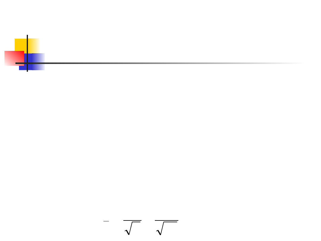
n

Y











Example 1



We compute confidence limits as
follows:



By definition

09

.

46

)

6592

.

0

(

)

960

.

1

(

8

.

44

L

is

limit

Upper

51

.

43

)

6592

.

0

(

)

960

.

1

(

8

.

44

L

is

limit

Lower

2

1





















95

.

0

09

.

46

51

.

43

P









Remark on example 1



Remember, that this is an unusual
case, in which we happen to know the
true mean of population ( = 45.5), and

hence we know that the confidence
limits enclose the mean.



We expect that 95% of such confidence
intervals obtained in repeated sampling
to include the parametric mean.

Example 1 – cont.



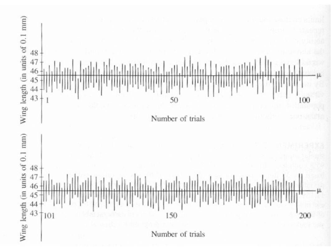
Lets try the experiment by
computer for 200 samples of 35
wing lengths each, computing
confidence limits of the parametric
mean by employing the parametric
standard error of mean,

6592

.

0

Y





Example 1 – cont.



Figure shows these 200 confidence
intervals plotted parallel to the
ordinate.

Example 1 – cont.



Of these, 194 (97.0%) cross the
parametric mean of the
population.

Remark

When we have set lower and upper limits to a

statistic, we imply that that the probability of this

interval covering the mean is equal to 0.95 or,

expressed in another way, that on the average, 95

out of 100 CIs similarly obtained would cover the

mean.

We

cannot state

that there is a probability of 0.95

that the true mean is contained within any

particular observed CLs, although this may seem

to be saying the same thing. The last statement is

incorrect because the true mean is a parameter;

hence it is a fixed value and is therefore either

inside or outside of the interval. It cannot be

inside a particular interval 95% of the time.

Choosing the sample size



To obtain a desired margin of error m,
just set this expression equal to m,
substitute the value of z* for your
desired confidence level, and solve for
the sample size n.



The confidence interval for a population
mean will have a specified margin of
error m when the sample size is

2

*















m

z

n



Example 2



What size should be the sample of,
to estimate the mean time of the
certain technical operation with
the max error equal to 20 secs if
we know that the variance equals
to 40

2

?

16

36

.

15

20

40

96

.

1

Error

z

n

0.95

-

1

seconds

20

Error

2

2

*











































Some cautions



The data must be an SRS from the

population.



The formula is not correct for probability

sampling designs more complex than an SRS.

(There are correct methods for more complex

designs.)



There is no correct method for inference from

data haphazardly collected with bias of

unknown size.



Outliers can have a large effect on the

confidence interval.

Some cautions, cont.



If the sample size is small and the
population is not normal, the true
confidence level will be different from the
value C used in computing the interval.



You must know the standard deviation σ
of the population.



The margin of error in a confidence
interval covers only random sampling
errors.

Inference for the Mean of
a Population



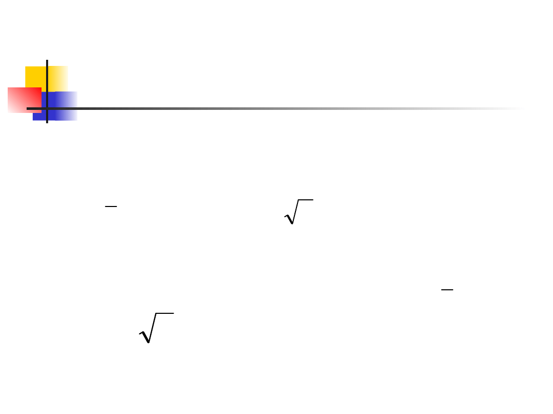
Suppose that we have a SRS of size n
from a normally distributed population
with mean μ and standard deviation σ.
The sample mean has a
distribution.



When σ is not known, we estimate it
with the sample standard deviation s,
and then we estimate the standard
deviation of by

x





n

N

/

,





x

n

s/

Standard Error



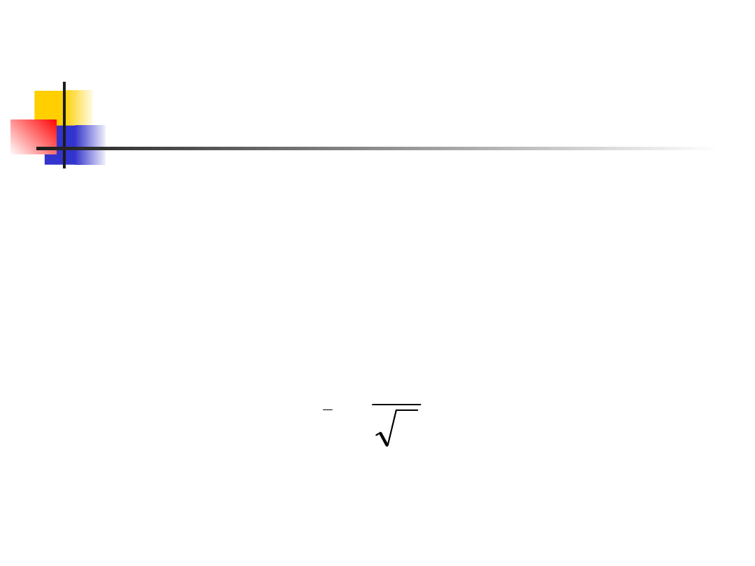
When a standard deviation of a
statistic is estimated from the
data, the result is called the
standard error of the statistic. The
standard error of the sample mean
is

n

s

SE

x



The t distribution



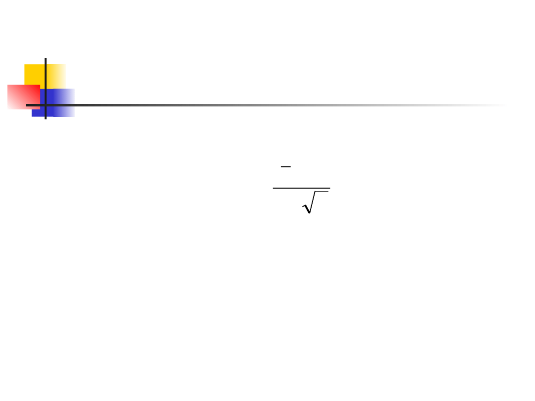
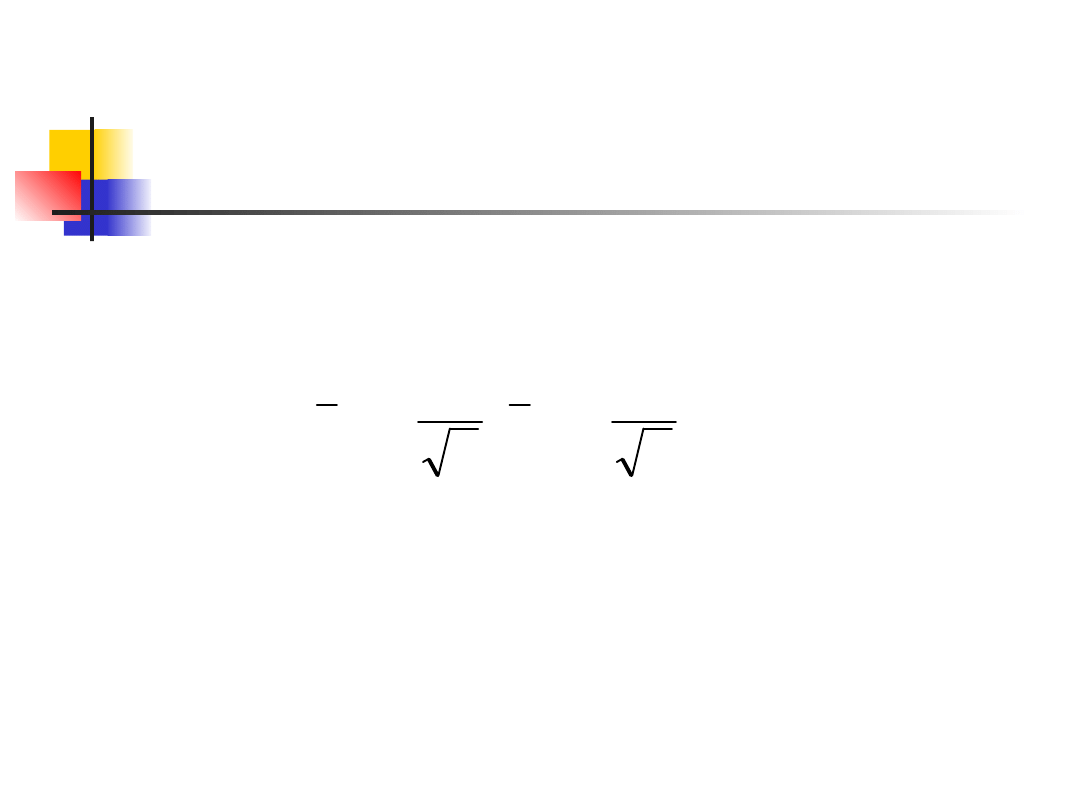
The standardized sample mean, or one-

sample z statistic,

is the basis of the z procedures for inference

about μ when σ is known. This statistic has a

N(0,1) distribution. When we substitute the

standard error for the standard deviation of

the sample mean, the statistic does NOT have

a normal distribution. It has a t distribution.

n

x

z

/









The t distribution, cont.



Suppose that an SRS of size n is drawn

from a population. Then the one-

sample t statistic

has the t distribution with n-1 degrees of

freedom.



There is a different t distribution for each

sample size.



A particular t distribution is specified by

giving the degrees of freedom.









,

N

n

s

x

t

/







The t distribution, cont.



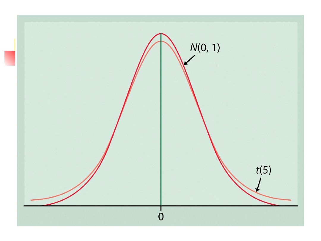
We use t(k) to stand for the t distribution with

k degrees of freedom.



The density curves of the t(k) distributions

are similar in shape to the standard normal

curve.



Symmetric about 0



Bell-shaped



Spread of the t distributions is a bit greater

than that of the standard normal distribution.



Due to the extra variability caused by substituting

the random variable s for the fixed parameter σ.

The t distribution, cont.



As the degrees of freedom k
increase, the t(k) density curve
approaches the N(0,1) curve ever
more closely.



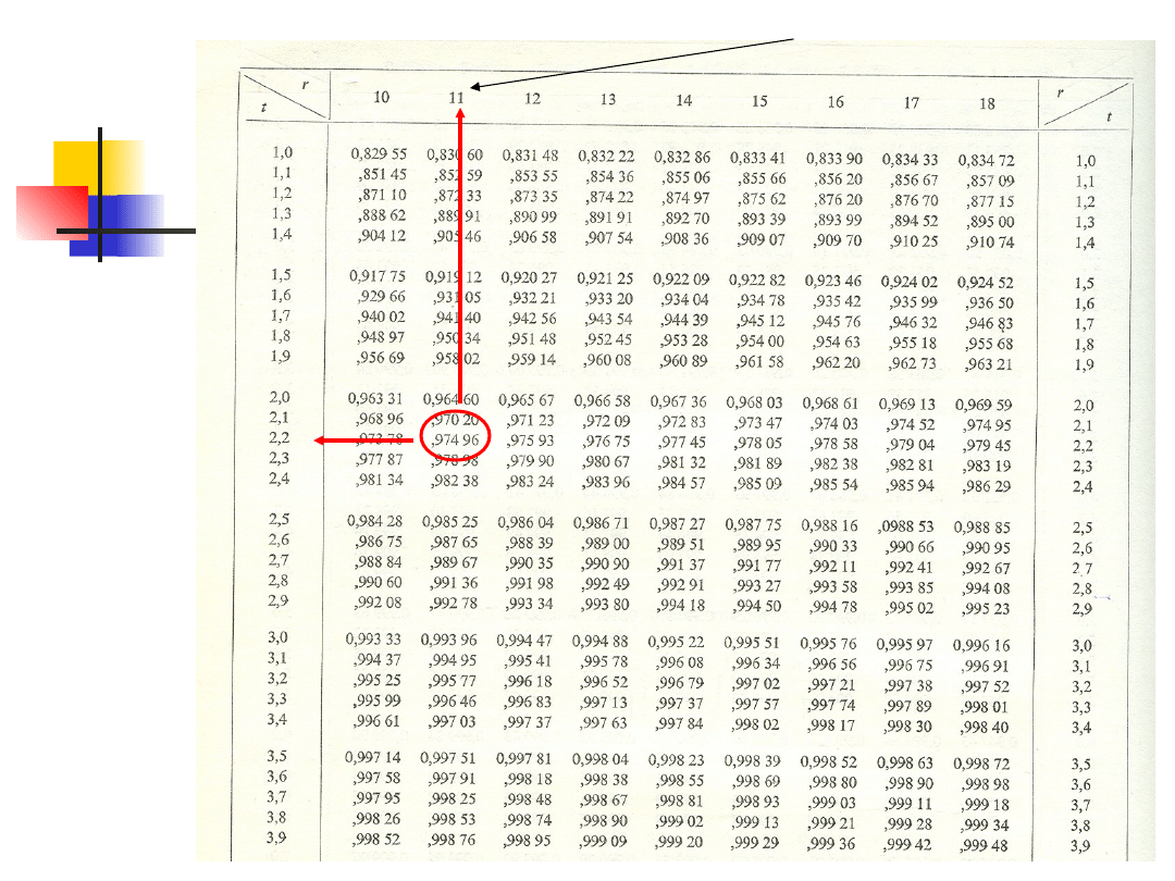
almost in every book on statistics
you can find a table that gives
critical values for the distributions.

The one-sample t
confidence interval



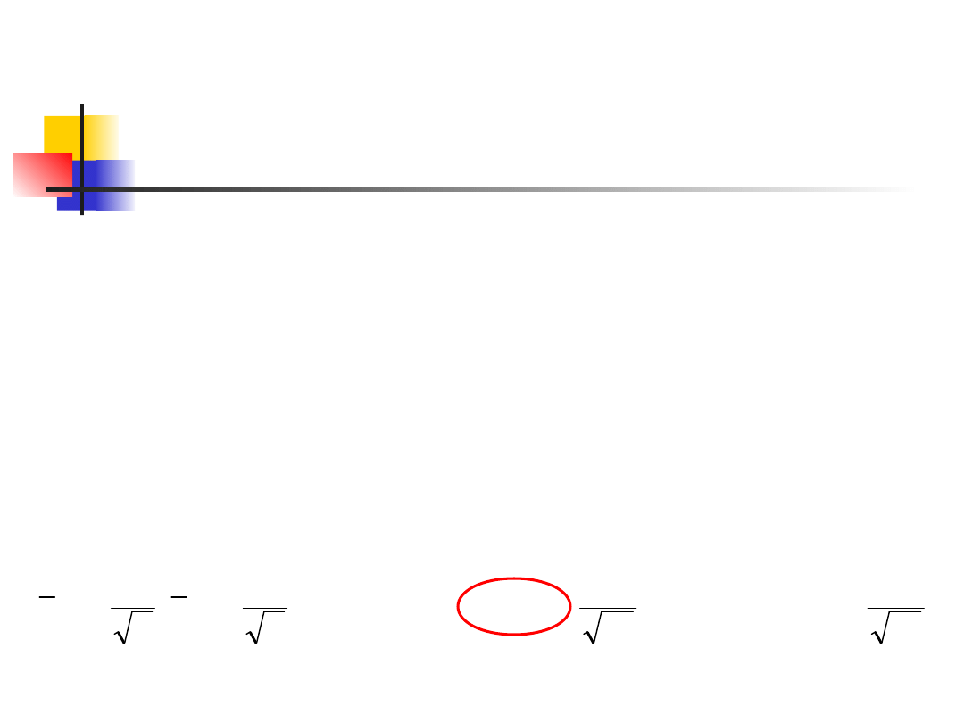
Suppose that an SRS of size n is drawn from a

population having unknown mean μ. A level C

confidence interval for μ is

where t* is the value for the t(n-1) density

curve with area C between –t* and t*. This

interval is exact when the population

distribution is normal and is approximately

correct for large n in other cases.

n

s

t

x

n

s

t

x

*

*

, 



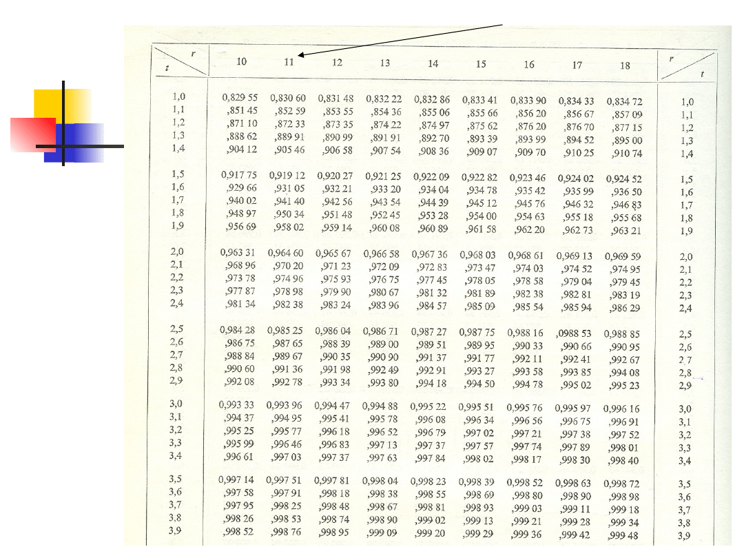
degree of freedom

The one-sample t
confidence interval -
example



Suppose that an SRS of size n is drawn from a
population having unknown mean μ.



[114, 123.3, 116.7, 129.0, 118, 124.6, 123.1,
117.4, 111, 121.7, 124.5, 130.5]



sample mean = 121.15



sample standard deviation = 5.89



critical t-value for 95% CI (11 degree of
freedom) = 2.2010





89

.

124

;

41

.

117

12

89

.

5

*

2010

.

2

15

.

121

;

12

89

.

5

*

2010

.

2

15

.

121

n

s

t

x

,

n

s

t

x

*

*







































95

%

2.5

%

2.5

%

degree of freedom

Example 3

Twenty-five femur lengths of

stem mothers of the aphid

Pemphigus populitransversus.

Measurements are in mm x 10

-1.

3.8

3.6

4.3

3.5

4.3

3.3

4.3

3.9

4.3

3.8

3.9

4.4

3.8

4.7

3.6

4.1

4.4

4.5

3.6

3.8

4.4

4.1

3.6

4.2

3.9

Example 3



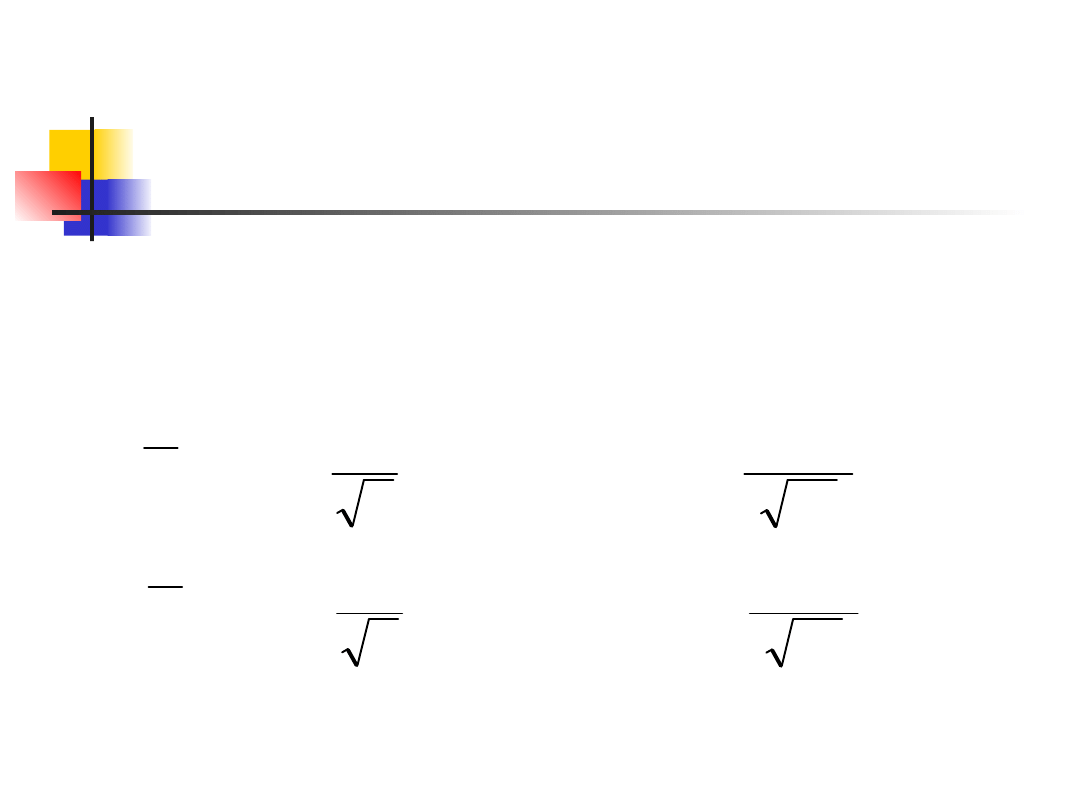
We calculate

and from t-tables we get

25

n

;

366

.

0

s

;

004

.

4

Y







797

.

2

t

01

.

0

for

064

.

2

t

05

.

0

for

24

,

01

.

0

24

,

05

.

0

















Example 3



The 95% CLs for the population
mean  are given by the

equations:

155

.

4

25

366

.

0

064

.

2

004

.

4

n

s

t

Y

L

853

.

3

25

366

.

0

064

.

2

004

.

4

n

s

t

Y

L

24

,

05

.

0

2

24

,

05

.

0

1

















































Example 3



The 99% CLs for the population
mean  are given by the

equations:

209

.

4

25

366

.

0

797

.

2

004

.

4

n

s

t

Y

L

799

.

3

25

366

.

0

797

.

2

004

.

4

n

s

t

Y

L

24

,

01

.

0

2

24

,

01

.

0

1

















































Confidence limits based on
sample statistics



We can use the same technique for
setting confidence limits to any
statistics, as long as the statistics
follows normal distribution.



This technique applies in an
approximate way to all the
statistics of the table on the next
slide.

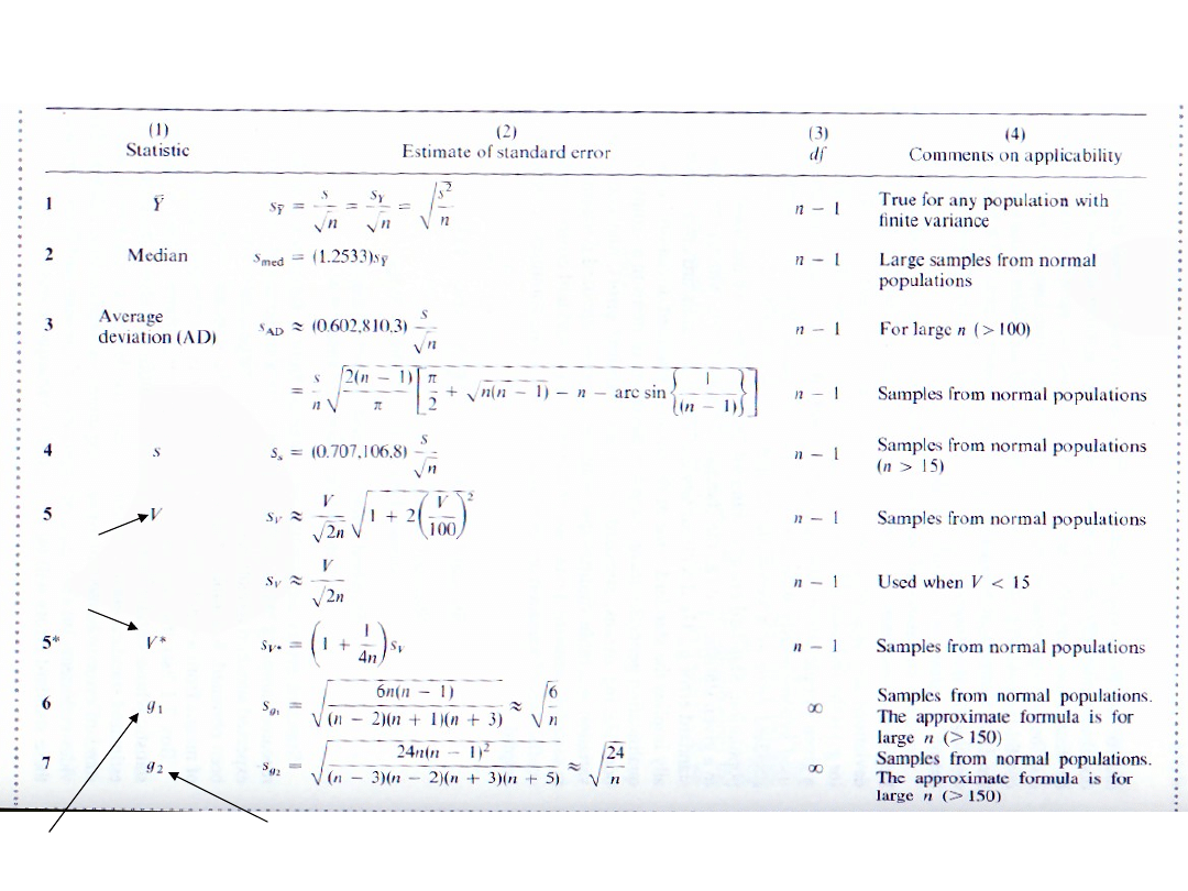
skewness

kurtosis

biased estimator

unbiased estimator

The chi-square distribution



The chi-square distribution is a
probability density function whose
values range from zero to positive
infinity.



Thus, unlike the normal distribution,
or t, the function approaches the 

2

axis asymptotically only at the right-
hand tail of the curve, not both.

The chi-square distribution



As in the case of t, there is not
merely one 

2

distribution, but one

distribution for each number of
degrees of freedom.



The function describing the 

2

distribution is complicated and will
not be given here.

The chi-square distribution



We can generate a 

2

distribution

from a population of standard
normal deviates.



We standardize a variable X

i

by

subjecting it to the operation









i

'
i

X

X

The chi-square distribution



Now imagine repeated samples of n
variates X

i

from a normal population

with mean  and standard deviation .



For each sample we transform every
variate X

i

to X

i’

.



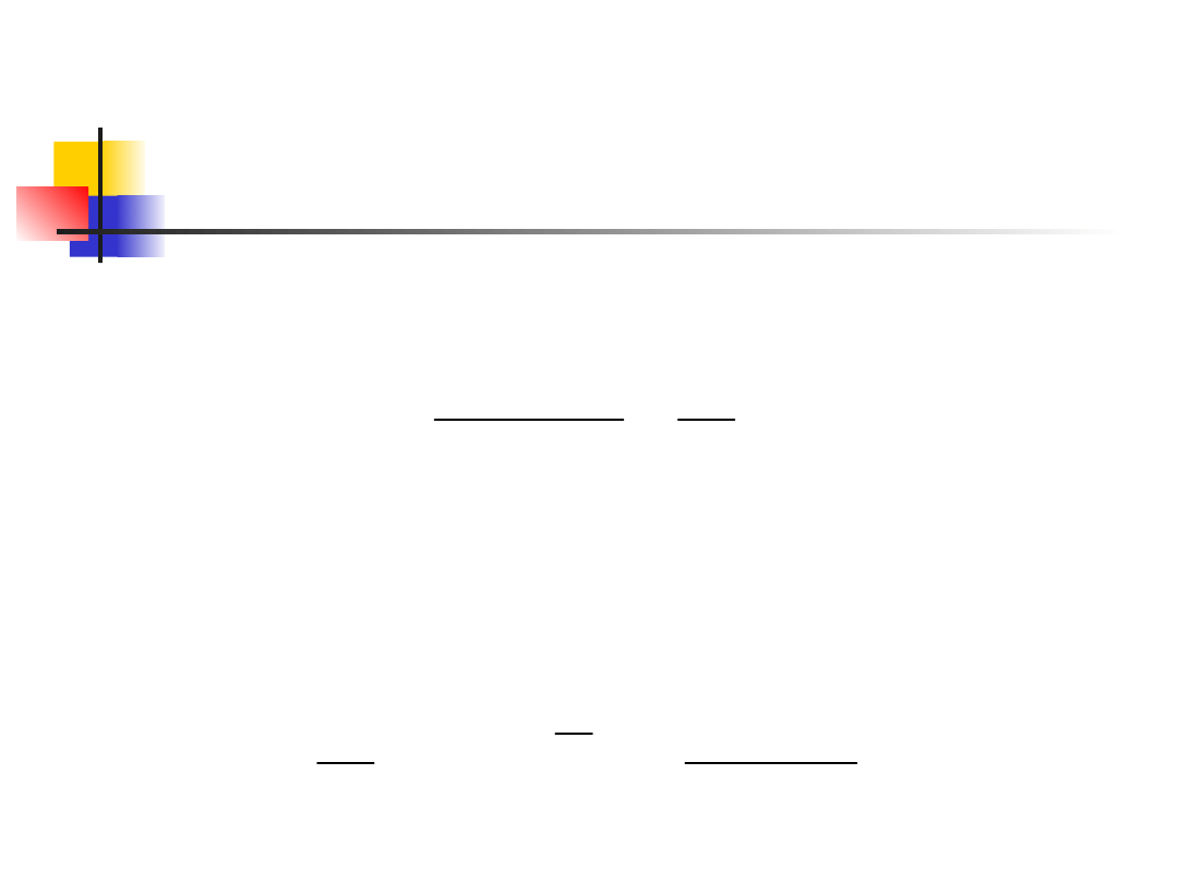
The quantities computed for
each sample will be distributed as a 

2

distribution with n degrees of freedom.



2

'
i

n

X

The chi-square distribution



We can rewrite



When we change the parametric
mean  to a sample mean, this

expression becomes

2

i

n

n

2

2

2

i

n

2

'
i

)

X

(

1

)

X

(

X























2

2

2

i

n

2

s

)

1

n

(

)

X

X

(

1













The chi-square distribution



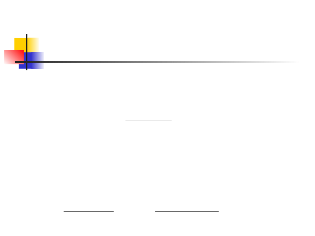
If we were sample repeatedly n

items from a normally distributed

population, the above quantity for

each sample would yield a 

2

distribution with

n-1

degrees of

freedom.



We have lost a degree of freedom

because we are now employing a

sample mean rather than

parametric mean.

The confidence limits for
variances



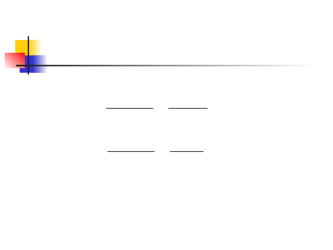
We can make the following

statement about the ratio



Simple algebraic manipulation of

the quantities in the inequality

within brackets yields









































1

s

)

1

n

(

P

2

]

1

n

[

),

2

/

(

2

2

2

]

1

n

[

)),

2

/

(

1

(















































1

s

)

1

n

(

s

)

1

n

(

P

2

]

1

n

[

)),

2

/

(

1

(

2

2

2

]

1

n

[

),

2

/

(

2

Example 4



Suppose we have a sample of 5
housefly wing lengths with a
sample variance of s

2

=13.52



If we wish to set 95% confidence
limits to the parametric variance,
we look up the values



They correspond to 11.143 and
0.484 respectively.

2

]

4

[

,

975

.

0

2

]

4

[

,

025

.

0

and





Example 4



The limits then become



This confidence interval is very

wide, but we must not forget that

the sample variance is, after all,

based on only 5 individuals.

74

.

111

0.484

54.08

52

.

13

4

L

4.85

11.143

54.08

52

.

13

4

L

2

]

4

[

,

975

.

0

2

2

]

4

[

,

025

.

0

1



















