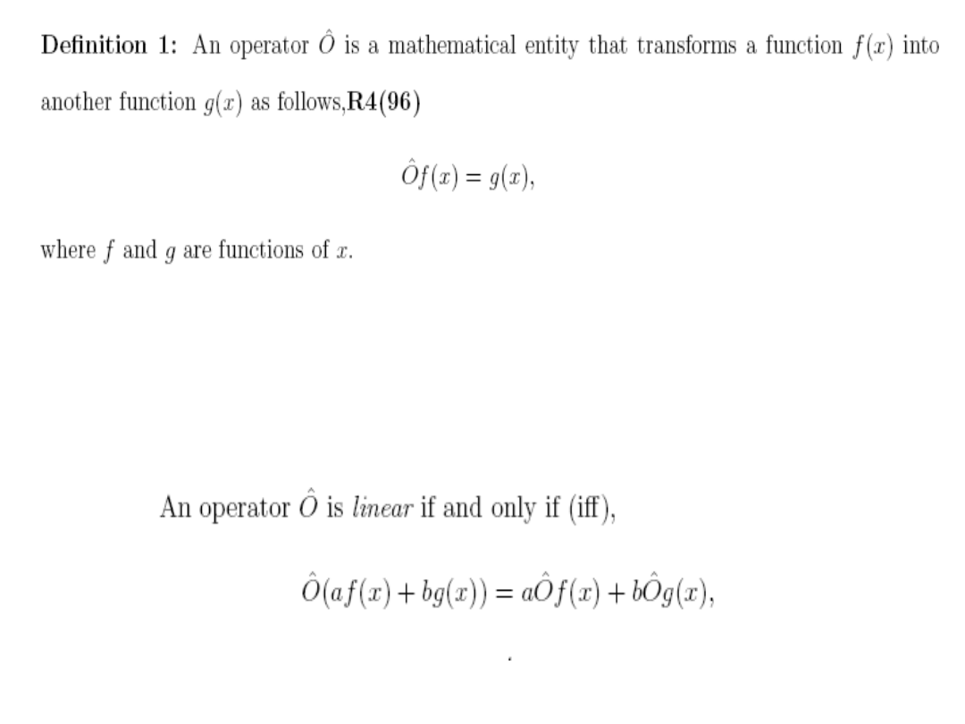
Eigenvalue Equations and
Operators
The Schrödinger equation
can be rewritten as
ˆ
H (x)E(x); ˆ
H =
h
2
2m
2
x
2
V(x)
where ˆ
H is the quantum mechanical Hamiltonian
ˆ
(operator
)(function
) (constant)(samefunction
)
(operator)(eigenfunction)
=(eigenvalue)(eigenfunction)
cos;
:
2
Some non-linear operators
:
For linear operators the following identities apply
:
(ˆ
A +ˆ
B )ˆ
C = ˆ
A ˆ
C +ˆ
B ˜
C ; ˆ
A (ˆ
B + ˆ
C ) = ˆ
A ˆ
B + ˆ
A ˆ
C
ˆ
A {f(x) g(x)} ˆ
A f(x) ˆ
A g(x)
ˆ
A {kf(x)}k ˆ
A f(x)
Some linear operators
:
x;x
2
;
d
dx
;
d
2
dx
2
Multiplicative
Differential

Operator
ˆ
A Function f
ˆ
A f(x)
d
dx
f f'
(x)
3 f 3f
cos() x cosx
x
x
Rules for operators
:
( ˆ
A ˆ
B )f(x) ˆ
A f(x) ˆ
B f(x): Sum of operators
( ˆ
A ˆ
B )f(x) ˆ
A f(x) ˆ
B f(x):Dif. of operators
15
3
3
)
15
3
(
3
)
5
(
3
)
5
(
ˆ
)
5
)(
3
ˆ
ˆ
(
ˆ
3
2
3
2
3
3
3
x
x
x
x
x
x
D
x
D
dx
d
=
D
Example

ˆ
A ˆ
B f(x) ˆ
A [ ˆ
B f(x)]:product of operators
We first operate on f with the operator '
ˆ
B '
on the right of the operator product,
and
then take the resulting function (
ˆ
B f) and
operate on it with the operator
ˆ
A on the left
of the operator product.
)
(
'
))
(
ˆ
(
ˆ
)
(
ˆ
ˆ
)
(
'
)
(
))
(
(
ˆ
)
(
ˆ
ˆ
ˆ
;
ˆ
x
xf
x
f
D
x
x
f
D
x
x
xf
x
f
x
xf
D
x
f
x
D
x
x
dx
d
=
D
Example
Operators do not necessarily obey the commutative law
:
ˆ
A ˆ
B ˆ
B ˆ
A 0: ˆ
A ˆ
B ˆ
B ˆ
A [ ˆ
A , ˆ
B ]0
Cummutator
:

Example: ˆ
A = X
2
; ˆ
B =
d
dx
ˆ
A ˆ
B f x
2
df
dx
: ˆ
B ˆ
A f =
d(x
2
f)
dx
2xf x
2
df
dx
[ˆ
A ,ˆ
B ]f 2xf
The square of an operator is defined as the product of
the operator with itself
: ˆ
A
2
= ˆ
A ˆ
A
Examples : ˆ
D =
d
dx
ˆ
D ˆ
D f(x)= ˆ
D (ˆ
D f(x))= ˆ
D f'(x)f"(x)
ˆ
D
2
d
2
dx
2
apply
rules
follow
the
where
etc.
,
C
,
B
,
A
operators
linear
with
dealing
be
shall
We
ˆ
ˆ
ˆ

Hermetian Operators
Hermetian Operators
Consider a system described by the state function
.
Let
F
^
be the operator representing the observable F
The average value of
F , or the expectation value is given by
<F>
=
*
F
^
d
A physical expectation value must be real
Thus :
<F> = <F>
*
F
^
d
*
F
^
d
=
(
F
^
d
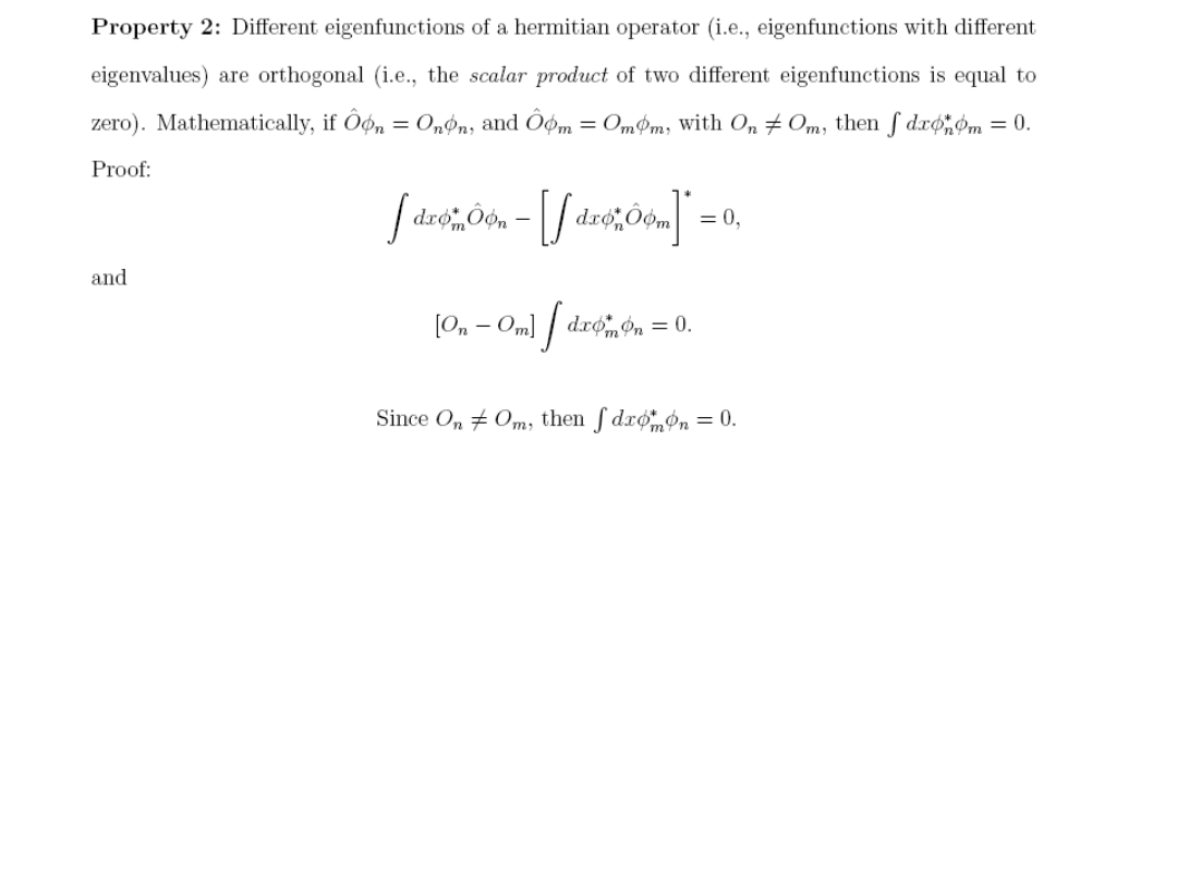
An operator that satisfy this condition is
Hermitian
One Definition of
Hermitian operator
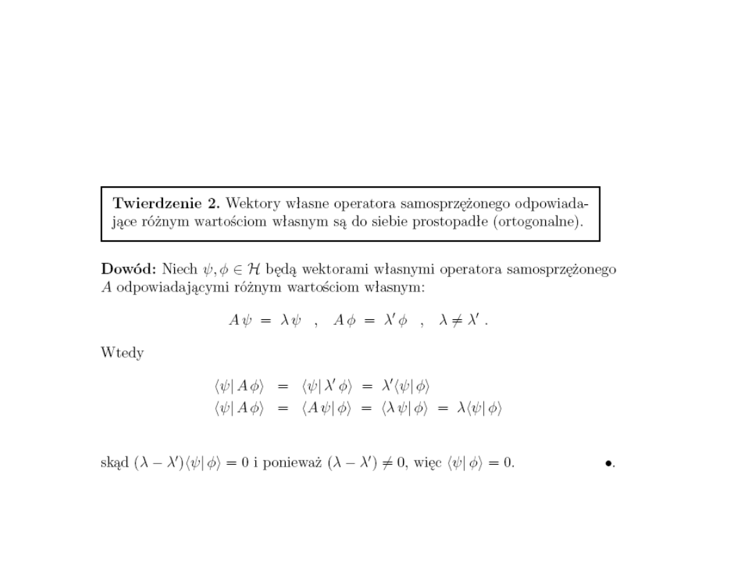

Funkcje własne odpowiadające tej samej wartości można ortogonalizować
(wartości własne zdegenerowane)
)
deg
(
,...,
2
,
1
ˆ
,
,
eneracji
krotno
śr
g
j
f
F
j
l
l
j
l
0
)
ˆ
(
,
j
l
l
f
F
j
i
j
l
i
l
l
l
l
l
l
l
l
l
l
l
i
l
l
g
j
j
l
j
l
i
l
d
itd
d
d
itd
x
x
N
x
N
)
-f
F
(
c
y
,
,
*
,
3
,
*
1
,
3,1
2
,
*
1
,
2,1
2
,
2
,
3
1
,
1
,
3
3
,
3
l,3
1
,
1
,
2
2
,
2
l,2
1
,
l,1
,
1
,
,
,
Wtedy
x
x
gdzie
.
)
(
)
(
wybierzmy
0
ˆ
wtedy
weźe

n
n
n
For an observable
with the corresponding
operator
ˆ
we have the eigenvalue equation
:
(IIIa). The meassurement of the quantity represented by
has as the o n l y outcome one of the values
n
n=1,2,3 ....
(IIIb). If the system is in a state described by
n
a meassurement of
will result in the
value
n

Examples of operators and their
eigenfunctions
Example Operator
Eigenfunction Eigenvalue
1
x
exp[ikx]
ik
2
2
x
exp[ikx]
k
2
3
2
x
coskx
k
2
4
2
x
sinkx
k
2
with the eigenfunction f and the eigenvalue k
**
.
**
ˆ
A f kf
ˆ
A (cf) k(cf)
sh
ow
Mu
st
Demonstrate that cf also is an eigenfunction to
ˆ
A
with the same eigenvalue k if c is a constant
proof:
ˆ
A is a Linear operator
ˆ
A (cf)cˆ
A f
*
ˆ
A
(cf) cˆ
A
f
operator
linear
a
be
A
Let ˆ
c is a constant
f is a function
e.g. A =
d
dx
ckf
f is an eigenfunction of
ˆ
A
Rearrangement of constant
factors and QED
k(cf)
we can solve the eigenvalue problem
ˆ
n
n
n
For any such operator
ˆ
We obtain
eigenfunctions
and eigenvalues
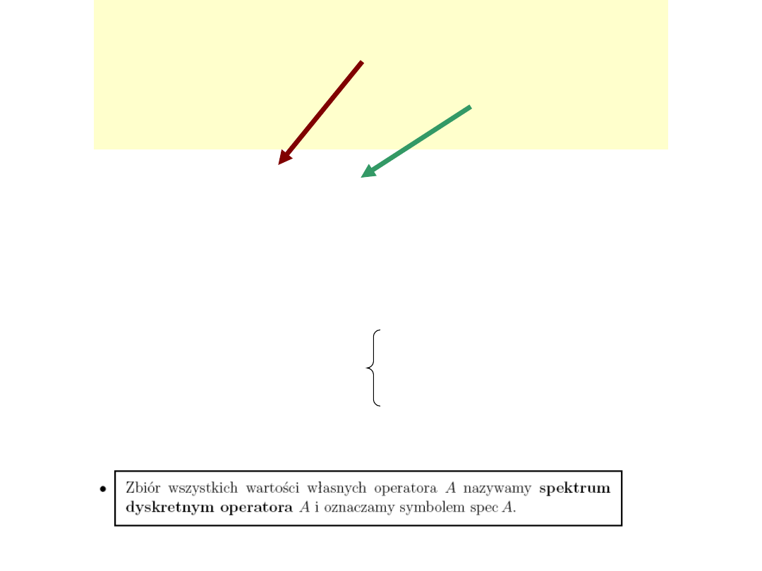
The only possible values that can arise from measurements
of the physical observable
are the eigenvalues
n
Postulate 3
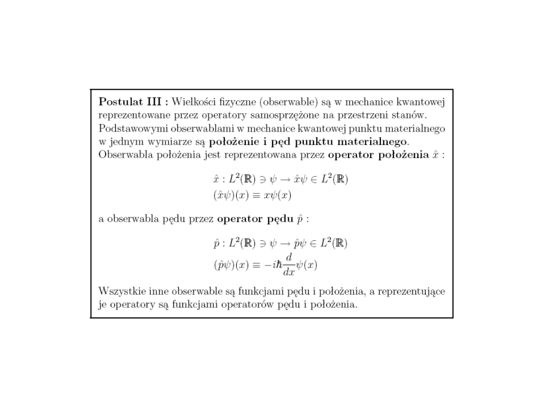
A linear operator
ˆ
A will have a set of
eigenfunctions f
n
(x) {n=1,2,3..etc}
and associated eigenvalues k
n
such that
:
The set of eigenfunction {f
n
(x),n 1..}
is orthonormal
:
f
i
(x)
*
all space
f
j
(x)dx
ij
ˆ
A f
n
(x) k
n
f
n
(x)
o if ij
1 if i=j
e
i
e
j
ij
ei
ei
ei
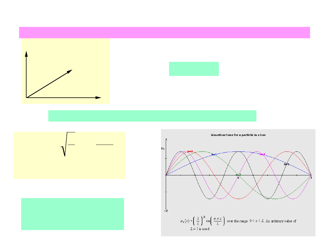
An example of an orthonormal set is the Cartesian unit vectors
An example of an orthonormal function set is
n
(x)=
1
L
sin
nx
L
n=1,2,3,4,5....
n
(x)
*
o
L
m
(x)
nm
That is, any function g(x) that
depends on the same variables
as the eigenfunctions can be written
g(x)= a
n
f
n
(x)
i=1
all
where
a
n
f
n
(x)
*
g(x)dx
all space
The set of eigenfunction {f
n
(x),n 1..}
forms a complete set.
ei
ei
ei
r
e
i
; i=1,2,3 form a complete set
For any vector
r
v
v (
r
v
r
e
1
)
r
e
1
(
r
v
r
e
2
)
r
e
2
(
r
v
r
e
3
)
r
e
3
Document Outline
- Slide 1
- Slide 2
- Slide 3
- Slide 4
- Slide 5
- Slide 6
- Slide 7
- Slide 8
- Slide 9
- Slide 10
- Slide 11
- Slide 12
- Slide 13
- Slide 14
- Slide 15
- Slide 16
- Slide 17
- Slide 18
- Slide 19
- Slide 20
- Slide 21
- Slide 22
- Slide 23
- Slide 24
- Slide 25
- Slide 26
- Slide 27
- Slide 28
- Slide 29
- Slide 30
- Slide 31
- Slide 32
- Slide 33
- Slide 34
- Slide 35
- Slide 36
- Slide 37
- Slide 38
- Slide 39
- Slide 40
Wyszukiwarka
Podobne podstrony:
03 Sejsmika04 plytkieid 4624 ppt
03 Odświeżanie pamięci DRAMid 4244 ppt
podrecznik 2 18 03 05
od Elwiry, prawo gospodarcze 03
Probl inter i kard 06'03
TT Sem III 14 03
03 skąd Państwo ma pieniądze podatki zus nfzid 4477 ppt
03 PODSTAWY GENETYKI
Wyklad 2 TM 07 03 09
03 RYTMY BIOLOGICZNE CZŁOWIEKAid 4197 ppt
Rada Ministrow oficjalna 97 03 (2)
Sys Inf 03 Manning w 06
KOMPLEKSY POLAKOW wykl 29 03 2012
więcej podobnych podstron