Elementary Statistics 10e TriolaE S CH05pp198 243

5-1

Overview

5-2

Random Variables

5-3

Binomial Probability Distributions

5-4

Mean, Variance, and Standard Deviation for the
Binomial Distribution

5-5

Poisson Probability Distributions

Discrete Probability
Distributions

TriolaE/S_CH05pp198-243 11/11/05 7:33 AM Page 198

C H A P T E R P R O B L E M

Can statistical methods
show that a jury selection
process is discriminatory?

After a defendant has been convicted of some crime,

appeals are sometimes filed on the grounds that the de-

fendant was not convicted by a jury of his or her peers.

One criterion is that the jury selection process should

result in jurors that represent the population of the re-

gion. In one notable case, Dr. Benjamin Spock, who

wrote the popular Baby and Child Care book, was con-

victed of conspiracy to encourage resistance to the draft

during the Vietnam War. His defense argued that Dr.

Spock was handicapped by the fact that all 12 jurors

were men. Women would have been more sympathetic,

because opposition to the war was greater among

women and Dr. Spock was so well known as a baby

doctor. A statistician testified that the presiding judge

had a consistently lower proportion of women jurors

than the other six judges in the same district.

Dr. Spock’s conviction was overturned for other rea-

sons, but federal court jurors are now supposed to be

randomly selected.

In 1972, Rodrigo Partida, a Mexican-American,

was convicted of burglary with intent to commit rape.

His conviction took place in Hidalgo County, which is

in Texas on the border with Mexico. Hidalgo County

had 181,535 people eligible for jury duty, and 80% of

them were Mexican-American. (Because the author re-

cently renewed his poetic license, he will use 80%

throughout this chapter instead of the more accurate

value of 79.1%.) Among 870 people selected for grand

jury duty, 39% (339) were Mexican-American. Partida’s

conviction was later appealed (Castaneda v. Partida)

on the basis of the large discrepancy between the 80%

of the Mexican-Americans eligible for grand jury duty

and the fact that only 39% of Mexican-Americans were

actually selected.

We will consider the Castaneda v. Partida issue in

this chapter. Here are key questions that will be addressed:

1. Given that Mexican-Americans constitute 80% of

the population, and given that Partida was con-

victed by a jury of 12 people with only 58% of

them (7 jurors) that were Mexican-American, can

we conclude that his jury was selected in a process

that discriminates against Mexican-Americans?

2. Given that Mexican-Americans constitute 80% of

the population of 181,535 and, over a period of 11

years, only 39% of those selected for grand jury

duty were Mexican-Americans, can we conclude

that the process of selecting grand jurors discrimi-

nated against Mexican-Americans? (We know that

because of random chance, samples naturally vary

somewhat from what we might theoretically

expect. But is the discrepancy between the 80%

rate of Mexican-Americans in the population and

the 39% rate of Mexican-Americans selected for

grand jury duty a discrepancy that is just too large

to be explained by chance?)

This example illustrates well the importance of a

basic understanding of statistical methods in the field of

law. Attorneys with no statistical background might not

be able to serve some of their clients well. The author

once testified in New York State Supreme Court and

observed from his cross-examination that a lack of un-

derstanding of basic statistical concepts can be very

detrimental to an attorney’s client.

TriolaE/S_CH05pp198-243 11/11/05 7:33 AM Page 199

200

Chapter 5

Discrete Probability Distributions

5-1

Overview

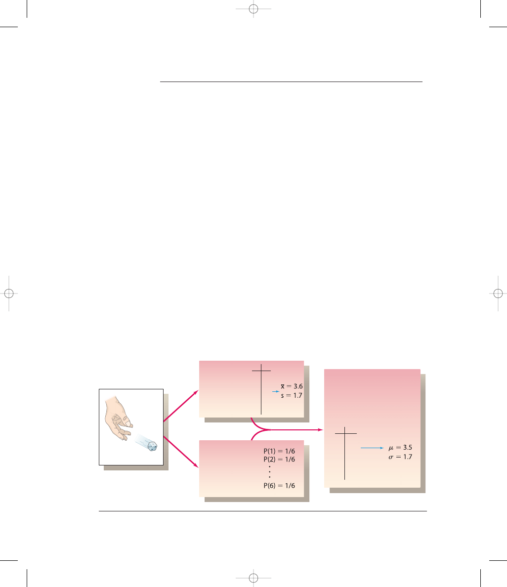
In this chapter we combine the methods of descriptive statistics presented in
Chapters 2 and 3 and those of probability presented in Chapter 4. Figure 5-1 pre-
sents a visual summary of what we will accomplish in this chapter. As the figure
shows, using the methods of Chapters 2 and 3, we would repeatedly roll the die to
collect sample data, which then can be described with graphs (such as a histogram
or boxplot), measures of center (such as the mean), and measures of variation
(such as the standard deviation). Using the methods of Chapter 4, we could find
the probability of each possible outcome. In this chapter we will combine those
concepts as we develop probability distributions that describe what will probably
happen instead of what actually did happen. In Chapter 2 we constructed fre-
quency tables and histograms using observed sample values that were actually
collected, but in this chapter we will construct probability distributions by pre-
senting possible outcomes along with the relative frequencies we expect. In this
chapter we consider discrete probability distributions, but Chapter 6 includes
continuous probability distributions.

The table at the extreme right in Figure 5-1 represents a probability distribu-

tion that serves as a model of a theoretically perfect population frequency distri-
bution. In essence, we can describe the relative frequency table for a die rolled an
infinite number of times. With this knowledge of the population of outcomes, we
are able to find its important characteristics, such as the mean and standard devia-
tion. The remainder of this book and the very core of inferential statistics are
based on some knowledge of probability distributions. We begin by examining the
concept of a random variable, and then we consider important distributions that
have many real applications.

Chapters

2 and 3

Chapter 4

Roll a die

Chapter 5

2 10
3

4 12
5 11
6 10

P(x)

1/6

Collect sample
data, then
get statistics
and graphs.

Find the
probability for
each outcome.

Create a theoretical model
describing how the experiment
is expected to behave, then
get its parameters.

Figure 5-1

Combining Descriptive Methods and Probabilities to Form a Theoretical Model of Behavior

TriolaE/S_CH05pp198-243 11/11/05 7:33 AM Page 200

5-2

Random Variables

201

5-2

Random Variables

Key Concept

This section introduces the important concept of a probability

distribution, which gives the probability for each value of a variable that is deter-
mined by chance. This section also includes procedures for finding the mean and
standard deviation for a probability distribution. In addition to the concept of a
probability distribution, particular attention should be given to methods for distin-
guishing between outcomes that are likely to occur by chance and outcomes that
are “unusual” in the sense that they are not likely to occur by chance.

We begin with the related concepts of random variable and probability distri-

bution.

Definitions

A random variable is a variable (typically represented by x) that has a single
numerical value, determined by chance, for each outcome of a procedure.

A probability distribution is a description that gives the probability for
each value of the random variable. It is often expressed in the format of a
graph, table, or formula.

Table 5-1

Probability Distribution:
Probabilities of Num-
bers of Mexican-
Americans on a Jury
of 12, Assuming That
Jurors Are Randomly
Selected from a Popu-
lation in Which 80%
of the Eligible People
are Mexican-Americans

(Mexican-

Americans)

P (x)

0.001

0.003

0.016

0.053

0.133

0.236

0.283

0.206

0.069

Definitions

A discrete random variable has either a finite number of values or a count-
able number of values, where “countable” refers to the fact that there might
be infinitely many values, but they can be associated with a counting process.

A continuous random variable has infinitely many values, and those val-
ues can be associated with measurements on a continuous scale without gaps
or interruptions.

EXAMPLE

Jury Selection

Twelve jurors are to be randomly

selected from a population in which 80% of the jurors are Mexican-
American. If we assume that jurors are randomly selected without

bias, and if we let

number of Mexican-American jurors among 12 jurors

then x is a random variable because its value depends on chance. The possible
values of x are 0, 1, 2, . . . , 12. Table 5-1 lists the values of x along with the
corresponding probabilities. Probability values that are very small, such as
0.000000123 are represented by 0

. (In Section 5-3 we will see how to find the

probability values, such as those listed in Table 5-1.) Because Table 5-1 gives
the probability for each value of the random variable x, that table describes a
probability distribution.

In Section 1-2 we made a distinction between discrete and continuous data. Ran-
dom variables may also be discrete or continuous, and the following two defini-
tions are consistent with those given in Section 1-2.

TriolaE/S_CH05pp198-243 11/11/05 7:33 AM Page 201

202

Chapter 5

Discrete Probability Distributions

2 8

(a) Discrete Random
Variable: Count of the
number of movie patrons.

(b) Continuous Random
Variable: The measured
voltage of a smoke detector
battery.

Voltmeter

Counter

Figure 5-2

Devices Used to Count and Measure Discrete and Continuous
Random Variables

Picking Lottery
Numbers

In a typical state lottery, you

select six different numbers.

After a random drawing, any

entries with the correct com-

bination share in the prize.

Since the winning numbers

are randomly selected, any

choice of six numbers will

have the same chance as any

other choice, but some com-

binations are better than

others. The combination of

1, 2, 3, 4, 5, 6 is a poor

choice because many people

tend to select it. In a Florida

lottery with a $105 million

prize, 52,000 tickets had 1, 2,

3, 4, 5, 6; if that combination

had won, the prize would

have been only $1000. It’s

wise to pick combinations

not selected by many others.

Avoid combinations that

form a pattern on the

entry card.

This chapter deals exclusively with discrete random variables, but the following
chapters will deal with continuous random variables.

EXAMPLES

The following are examples of discrete and continuous random

variables.

Let x

the number of eggs that a hen lays in a day. This is a discrete ran-

dom variable because its only possible values are 0, or 1, or 2, and so on.
No hen can lay 2.343115 eggs, which would have been possible if the data
had come from a continuous scale.

The count of the number of statistics students present in class on a given
day is a whole number and is therefore a discrete random variable. The
counting device shown in Figure 5-2(a) is capable of indicating only a fi-
nite number of values, so it is used to obtain values for a discrete random
variable.

Let x

the amount of milk a cow produces in one day. This is a continuous

random variable because it can have any value over a continuous span.
During a single day, a cow might yield an amount of milk that can be any
value between 0 gallons and 5 gallons. It would be possible to get 4.123456
gallons, because the cow is not restricted to the discrete amounts of 0, 1, 2,
3, 4, or 5 gallons.

TriolaE/S_CH05pp198-243 11/11/05 7:33 AM Page 202

5-2

Random Variables

203

robability

0.3

0.2

0.1

9 10 11 12

Probability Histogram for Number of

Mexican-American Jurors Among 12

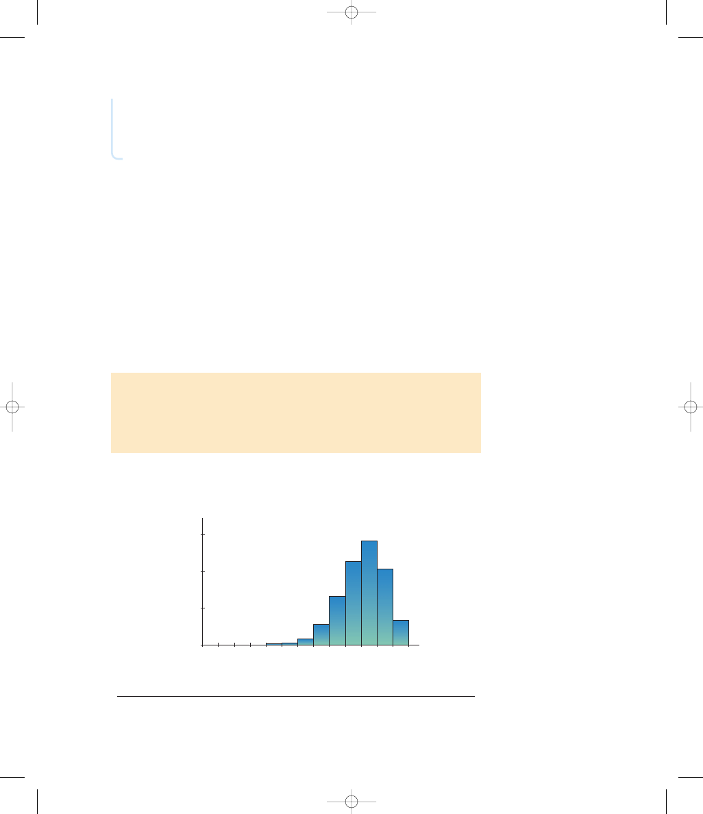
Figure 5-3

Probability Histogram for Number of Mexican-American Jurors Among
12 Jurors

The first requirement comes from the simple fact that the random variable x

represents all possible events in the entire sample space, so we are certain (with
probability 1) that one of the events will occur. (In Table 5-1, the sum of the

The measure of voltage for a particular smoke detector battery can be any
value between 0 volts and 9 volts. It is therefore a continuous random vari-
able. The voltmeter shown in Figure 5-2(b) is capable of indicating values
on a continuous scale, so it can be used to obtain values for a continuous
random variable.

Graphs

There are various ways to graph a probability distribution, but we will consider only
the probability histogram. Figure 5-3 is a probability histogram that is very similar
to the relative frequency histogram discussed in Chapter 2, but the vertical scale
shows probabilities instead of relative frequencies based on actual sample results.

In Figure 5-3, note that along the horizontal axis, the values of 0, 1, 2, . . . ,

12 are located at the centers of the rectangles. This implies that the rectangles
are each 1 unit wide, so the areas of the rectangles are 0

, 0, 0, 0, 0.001,

0.003, . . . , 0.069. The areas of these rectangles are the same as the probabilities
in Table 5-1. We will see in Chapter 6 and future chapters that such a correspon-
dence between area and probability is very useful in statistics.

Every probability distribution must satisfy each of the following two re-

quirements.

Requirements for a Probability Distribution

P(x)

where x assumes all possible values. (That is, the sum of
all probabilities must be 1.)

P(x) 1

for every individual value of x. (That is, each probability
value must be between 0 and 1 inclusive.)

TriolaE/S_CH05pp198-243 11/11/05 7:33 AM Page 203

204

Chapter 5

Discrete Probability Distributions

Table 5-2

Probabilities for a
Random Variable

P(x)

0.2

0.5

0.4

0.3

probabilities is 1, but in other cases values such as 0.999 or 1.001 are acceptable
because they result from rounding errors.) Also, the probability rule stating 0

P(x)

1 for any event A implies that P(x) must be between 0 and 1 for any value

of x. Because Table 5-1 does satisfy both of the requirements, it is an example of a
probability distribution. A probability distribution may be described by a table,
such as Table 5-1, or a graph, such as Figure 5-3, or a formula.

EXAMPLE

Does Table 5-2 describe a probability distribution?

SOLUTION

To be a probability distribution, P(x) must satisfy the preceding

two requirements. But

SP(x)

P(0) P(1) P(2) P(3)
0.2 0.5 0.4 0.3
1.4 [showing that SP(x) 1]

Because the first requirement is not satisfied, we conclude that Table 5-2 does
not describe a probability distribution.

EXAMPLE

Does P(x)

x 3 (where x can be 0, 1, or 2) determine a proba-

bility distribution?

SOLUTION

For the given function we find that P(0)

0 3, P(1) 1 3 and

P(2)

2 3, so that

Each of the P(x) values is between 0 and 1.

Because both requirements are satisfied, the P(x) function given in this exam-
ple is a probability distribution.

Mean, Variance, and Standard Deviation

In Chapter 2 we described the following important characteristics of data (which
can be remembered with the mnemonic of CVDOT for “Computer Viruses
Destroy Or Terminate”): (1) center; (2) variation; (3) distribution; (4) outliers;
and (5) time (changing characteristics of data over time). The probability his-
togram can give us insight into the nature or shape of the distribution. Also, we
can often find the mean, variance, and standard deviation of data, which provide
insight into the other characteristics. The mean, variance, and standard deviation
for a probability distribution can be found by applying Formulas 5-1, 5-2, 5-3,
and 5-4.

Formula 5-1

Mean for a probability distribution

Formula 5-2

Variance for a probability distribution

Formula 5-3

Variance for a probability distribution

Formula 5-4

Standard deviation for a probability
distribution

s 5 2S

? Psxd

4 2 m

5 S

? Psxd

4 2 m

5 S

3sx 2 md

? Psxd

m 5 S

3x ? Psxd4

SPsxd 5

5 1

TriolaE/S_CH05pp198-243 11/11/05 7:33 AM Page 204

5-2

Random Variables

205

It is sometimes necessary to use a different rounding rule because of special cir-

cumstances, such as results that require more decimal places to be meaningful. For
example, with four-engine jets the mean number of jet engines working successfully
throughout a flight is 3.999714286, which becomes 4.0 when rounded to one more
decimal place than the original data. Here, 4.0 would be misleading because it sug-
gests that all jet engines always work successfully. We need more precision to cor-
rectly reflect the true mean, such as the precision in the number 3.999714.

Identifying

Unusual Results with the

Range Rule of Thumb

The range rule of thumb (discussed in Section 3-3) may also be helpful in inter-
preting the value of a standard deviation. According to the range rule of thumb,
most values should lie within 2 standard deviations of the mean; it is unusual for a
value to differ from the mean by more than 2 standard deviations. (The use of 2
standard deviations is not an absolutely rigid value, and other values such as 3

Caution: Evaluate

by first squaring each value of x, then multiplying

each square by the corresponding probability P(x), then adding.

Rationale for Formulas 5-1 through 5-4

Instead of blindly accepting and using formulas, it is much better to have some un-
derstanding of why they work. Formula 5-1 accomplishes the same task as the for-
mula for the mean of a frequency table. (Recall that f represents class frequency
and N represents population size.) Rewriting the formula for the mean of a fre-
quency table so that it applies to a population and then changing its form, we get

In the fraction f N, the value of f is the frequency with which the value x occurs
and N is the population size, so f N is the probability for the value of x.

Similar reasoning enables us to take the variance formula from Chapter 3 and

apply it to a random variable for a probability distribution; the result is Formula 5-2.
Formula 5-3 is a shortcut version that will always produce the same result as For-
mula 5-2. Although Formula 5-3 is usually easier to work with, Formula 5-2 is
easier to understand directly. Based on Formula 5-2, we can express the standard
deviation as

or as the equivalent form given in Formula 5-4.

When applying Formulas 5-1 through 5-4, use this rule for rounding results.

s 5 2S

3sx 2 md

? Psxd

m 5

Ssƒ ? xd

ƒ ? x

x ?

3x # Psxd4

S[x

# Psxd]

Round-off Rule for M, S, and S

Round results by carrying one more decimal place than the number of deci-
mal places used for the random variable x. If the values of x are integers,
round

and

to one decimal place.

m, s,

TriolaE/S_CH05pp198-243 11/11/05 7:33 AM Page 205

206

Chapter 5

Discrete Probability Distributions

could be used instead.) We can therefore identify “unusual” values by determining
that they lie outside of these limits:

Range Rule of Thumb
maximum usual value

minimum usual value

EXAMPLE

Table 5-1 describes the probability distribution for the number

of Mexican-Americans among 12 randomly selected jurors in Hidalgo
County, Texas. Assuming that we repeat the process of randomly selecting
12 jurors and counting the number of Mexican-Americans each time, find
the mean number of Mexican-Americans (among 12), the variance, and the
standard deviation. Use those results and the range rule of thumb to find the
maximum and minimum usual values. Based on the results, determine
whether a jury consisting of 7 Mexican-Americans among 12 jurors is usual
or unusual.

SOLUTION

In Table 5-3, the two columns at the left describe the probability

distribution given earlier in Table 5-1, and we create the three columns at the
right for the purposes of the calculations required.

Using Formulas 5-1 and 5-3 and the table results, we get

9.598 9.6

(rounded)

94.054 9.598

1.932396 1.9

(rounded)

The standard deviation is the square root of the variance, so

(rounded)

We now know that when randomly selecting 12 jurors, the mean number of
Mexican-Americans is 9.6, the variance is 1.9 “Mexican-Americans
squared,’’ and the standard deviation is 1.4 Mexican-Americans. Using the
range rule of thumb, we can now find the maximum and minimum usual val-
ues as follows:

maximum usual value:

9.6 2(1.4) 12.4

minimum usual value:

9.6 2(1.4) 6.8

INTERPRETATION

Based on these results, we conclude that for groups of

12 jurors randomly selected in Hidalgo County, the number of Mexican-
Americans should usually fall between 6.8 and 12.4. If a jury consists of 7
Mexican-Americans, it would not be unusual and would not be a basis for a
charge that the jury was selected in a way that it discriminates against Mexican-
Americans. (The jury that convicted Roger Partida included 7 Mexican-
Americans, but the charge of an unfair selection process was based on the
process for selecting grand juries, not the specific jury that convicted him.)

m 2 2s

m 1 2s

s 5 21.932396 5 1.4

5 S

? Psxd

4 2 m

m 5 S

3x ? Psxd4

m 2 2s

m 1 2s

TriolaE/S_CH05pp198-243 11/11/05 7:33 AM Page 206

5-2

Random Variables

207

Table 5-3

Calculating

and

for a Probability Distribution

P(x)

0.000

0.001

0.004

0.016

0.003

0.015

0.075

0.016

0.096

0.576

0.053

0.371

2.597

0.133

1.064

8.512

0.236

2.124

19.116

0.283

2.830

100

28.300

0.206

2.266

121

24.926

0.069

0.828

144

9.936

Total

9.598

94.054

P(x)

, s,

Identifying

Unusual Results with Probabilities

Strong recommendation: Take time to carefully read and understand the rare event
rule and the paragraph that follows it. This brief discussion presents an extremely
important approach used often in statistics.

Rare Event Rule

If, under a given assumption (such as the assumption that a coin is fair), the prob-
ability of a particular observed event (such as 992 heads in 1000 tosses of a coin)
is extremely small, we conclude that the assumption is probably not correct.

Probabilities can be used to apply the rare event rule as follows:

Using Probabilities to Determine When Results Are Unusual

●

Unusually high number of successes: x successes among n trials is an
unusually high number of successes if P(x or more)

0.05.*

●

Unusually low number of successes: x successes among n trials is an
unusually low number of successes if P(x or fewer)

0.05.*

Suppose you were flipping a coin to determine whether it favors heads, and

suppose 1000 tosses resulted in 501 heads. This is not evidence that the coin

*The value of 0.05 is commonly used, but is not absolutely rigid. Other values, such as 0.01, could
be used to distinguish between events that can easily occur by chance and events that are very un-
likely to occur by chance.

TriolaE/S_CH05pp198-243 11/11/05 7:33 AM Page 207

208

Chapter 5

Discrete Probability Distributions

favors heads, because it is very easy to get a result like 501 heads in 1000 tosses
just by chance. Yet, the probability of getting exactly 501 heads in 1000 tosses is
actually quite small: 0.0252. This low probability reflects the fact that with 1000
tosses, any specific number of heads will have a very low probability. However,
we do not consider 501 heads among 1000 tosses to be unusual, because the prob-
ability of getting at least 501 heads is high: 0.487.

EXAMPLE

Jury Selection

If 80% of those eligible for jury

duty in Hidalgo County are Mexican-American, then a jury of 12
randomly selected people should have around 9 or 10 who are

Mexican-American. (The mean number of Mexican-Americans on juries
should be 9.6.) Is 7 Mexican-American jurors among 12 an unusually low
number? Does the selection of only 7 Mexican-Americans among 12 jurors
suggest that there is discrimination in the selection process?

SOLUTION

We will use the criterion that 7 Mexican-Americans among 12

jurors is unusually low if P(7 or fewer Mexican-Americans)

0.05. If we re-

fer to Table 5-1, we get this result:

P(7 or fewer Mexican-Americans among 12 jurors)

P(7 or 6 or 5 or 4 or 3 or 2 or 1 or 0)
P(7) P(6) P(5) P(4) P(3) P(2) P(1) P(0)
0.053 0.016 0.003 0.001 0 0 0 0
0.073

INTERPRETATION

Because the probability 0.073 is greater than 0.05, we

conclude that the result of 7 Mexican-Americans is not unusual. There is a
high likelihood (0.073) of getting 7 Mexican-Americans by random chance.
(Only a probability of 0.05 or less would indicate that the event is unusual.) No
court of law would rule that under these circumstances, the selection of only 7
Mexican-American jurors is discriminatory.

Expected Value

The mean of a discrete random variable is the theoretical mean outcome for in-
finitely many trials. We can think of that mean as the expected value in the sense
that it is the average value that we would expect to get if the trials could continue
indefinitely. The uses of expected value (also called expectation, or mathematical
expectation) are extensive and varied, and they play a very important role in an
area of application called decision theory.

Definition

The expected value of a discrete random variable is denoted by E, and it rep-
resents the average value of the outcomes. It is obtained by finding the value
of

3x ? Psxd4

3x ? Psxd4.

TriolaE/S_CH05pp198-243 11/11/05 7:33 AM Page 208

5-2

Random Variables

209

Table 5-4

Kentucky Pick 4 Lottery

Event

P(x)

Lose

0.9999

$0.9999

Gain (net)

$4999

0.0001

$0.4999

Total

$0.50

(or

50¢)

From Formula 5-1 we see that E

That is, the mean of a discrete random

variable is the same as its expected value. See Table 5-3 and note that when se-
lecting 12 jurors from a population in which 80% of the people are Mexican-
Americans, the mean number of Mexican-Americans is 9.6, so it follows that the
expected value of the number of Mexican-Americans is also 9.6.

EXAMPLE

Kentucky Pick 4 Lottery

If you bet $1 in Kentucky’s Pick

4 lottery game, you either lose $1 or gain $4999. (The winning prize is $5000,
but your $1 bet is not returned, so the net gain is $4999.) The game is played by
selecting a four-digit number between 0000 and 9999. If you bet $1 on 1234,
what is your expected value of gain or loss?

SOLUTION

For this bet, there are two outcomes: You either lose $1 or you

gain $4999. Because there are 10,000 four-digit numbers and only one of them
is the winning number, the probability of losing is 9,999 10,000 and the prob-
ability of winning is 1 10,000. Table 5-4 summarizes the probability distribu-
tion, and we can see that the expected value is E

50¢.

INTERPRETATION

In any individual game, you either lose $1 or have a net

gain of $4999, but the expected value shows that in the long run, you can ex-
pect to lose an average of 50¢ for each $1 bet. This lottery might have some
limited entertainment value, but it is definitely an extremely poor financial
investment.

In this section we learned that a random variable has a numerical value associ-

ated with each outcome of some random procedure, and a probability distribution
has a probability associated with each value of a random variable. We examined
methods for finding the mean, variance, and standard deviation for a probability
distribution. We saw that the expected value of a random variable is really the
same as the mean. Finally, an extremely important concept of this section is the
use of probabilities for determining when outcomes are unusual.

5-2

BASIC SKILLS AND CONCEPTS

Statistical Literacy and Critical Thinking

Probability Distribution

Consider the trial of rolling a single die, with outcomes of

1, 2, 3, 4, 5, 6. Construct a table representing the probability distribution.

TriolaE/S_CH05pp198-243 11/11/05 7:33 AM Page 209

210

Chapter 5

Discrete Probability Distributions

Probability Distribution

One of the requirements of a probability distribution is that

the sum of the probabilities must be 1 (with a small amount of leeway allowed for
rounding errors). What is the justification for this requirement?

Probability Distribution

A professional gambler claims that he has loaded a die so

that the outcomes of 1, 2, 3, 4, 5, 6 have corresponding probabilities of 0.1, 0.2, 0.3,
0.4, 0.5, and 0.6. Can he actually do what he has claimed? Is a probability distribution
described by listing the outcomes along with their corresponding probabilities?

Expected Value

A researcher calculates the expected value for the number of girls in

five births. He gets a result of 2.5. He then rounds the result to 3, saying that it is not
possible to get 2.5 girls when five babies are born. Is this reasoning correct?

Identifying Discrete and Continuous Random Variables. In Exercises 5 and 6, identify
the given random variable as being discrete or continuous.

5. a. The height of a randomly selected giraffe living in Kenya

b. The number of bald eagles located in New York State
c. The exact time it takes to evaluate 27

72.

d. The number of textbook authors now sitting at a computer
e. The number of statistics students now reading a book

6. a. The cost of conducting a genetics experiment

b. The number of supermodels who ate pizza yesterday
c. The exact life span of a kitten
d. The number of statistics professors who read a newspaper each day
e. The weight of a feather

Identifying Probability Distributions. In Exercises 7–12, determine whether a probabil-
ity distribution is given. In those cases where a probability distribution is not described,
identify the requirements that are not satisfied. In those cases where a probability distri-
bution is described, find its mean and standard deviation.

Genetic Disorder

Three males with an X-linked genetic disorder

have one child each. The random variable x is the number of
children among the three who inherit the X-linked genetic
disorder.

Numbers of Girls

A researcher reports that when groups of four

children are randomly selected from a population of couples
meeting certain criteria, the probability distribution for the num-
ber of girls is as given in the accompanying table.

Genetics Experiment

A genetics experiment involves offspring

peas in groups of four. A researcher reports that for one group,
the number of peas with white flowers has a probability distribu-
tion as given in the accompanying table.

P(x)

0.4219

0.1406

0.0156

P(x)

0.502

0.365

0.098

0.011

0.001

P(x)

0.04

0.16

0.80

0.16

0.04

TriolaE/S_CH05pp198-243 11/11/05 7:33 AM Page 210

5-2

Random Variables

211

10.

Mortality Study

For a group of four men, the probability distri-

bution for the number x who live through the next year is as
given in the accompanying table.

11.

Number of Games in a Baseball World Series

Based on past re-

sults found in the Information Please Almanac, there is a
0.1818 probability that a baseball World Series contest will last
four games, a 0.2121 probability that it will last five games, a
0.2323 probability that it will last six games, and a 0.3737 probability that it will
last seven games. Is it unusual for a team to “sweep” by winning in four games?

12.

Brand Recognition

In a study of brand recognition of Sony, groups of four con-

sumers are interviewed. If x is the number of people in the group who recognize the
Sony brand name, then x can be 0, 1, 2, 3, or 4, and the corresponding probabilities
are 0.0016, 0.0250, 0.1432, 0.3892, and 0.4096. Is it unusual to randomly select
four consumers and find that none of them recognize the brand name of Sony?

13.

Determining Whether a Jury Selection Process Discriminates

Assume that 12 jurors

are randomly selected from a population in which 80% of the people are Mexican-
Americans. Refer to Table 5-1 and find the indicated probabilities.
a. Find the probability of exactly 5 Mexican-Americans among 12 jurors.
b. Find the probability of 5 or fewer Mexican-Americans among 12 jurors.
c. Which probability is relevant for determining whether 5 jurors among 12 is unusu-

ally low: the result from part (a) or part (b)?

d. Does 5 Mexican-Americans among 12 jurors suggest that the selection process

discriminates against Mexican-Americans? Why or why not?

14.

Determining Whether a Jury Selection Process Discriminates

Assume that 12 jurors

are randomly selected from a population in which 80% of the people are Mexican-
Americans. Refer to Table 5-1 and find the indicated probabilities.
a. Find the probability of exactly 6 Mexican-Americans among 12 jurors.
b. Find the probability of 6 or fewer Mexican-Americans among 12 jurors.
c. Which probability is relevant for determining whether 6 jurors among 12 is unusu-

ally low: the result from part (a) or part (b)?

d. Does 6 Mexican-Americans among 12 jurors suggest that the selection process

discriminates against Mexican-Americans? Why or why not?

15.

Determining Whether a Jury Selection Process Discriminates

Assume that 12 jurors

are randomly selected from a population in which 80% of the people are Mexican-
Americans. Refer to Table 5-1 and find the indicated probability.
a. Using the probability values in Table 5-1, find the probability value that should be

used for determining whether the result of 8 Mexican-Americans among 12 jurors
is unusually low.

b. Does the result of 8 Mexican-American jurors suggest that the selection process

discriminates against Mexican-Americans? Why or why not?

16.

Determining Whether a Jury Selection Process Is Biased

Assume that 12 jurors are

randomly selected from a population in which 80% of the people are Mexican-
Americans. Refer to Table 5-1 and find the indicated probability.
a. Using the probability values in Table 5-1, find the probability value that should be

used for determining whether the result of 11 Mexican-Americans among 12 jurors
is unusually high.

b. Does the selection of 11 Mexican-American jurors suggest that the selection pro-

cess favors Mexican-Americans? Why or why not?

P(x)

0.0000

0.0001

0.0006

0.0387

0.9606

TriolaE/S_CH05pp198-243 11/11/05 7:33 AM Page 211

212

Chapter 5

Discrete Probability Distributions

17.

Expected Value in Roulette

When you give the Venetian casino in Las Vegas $5 for a

bet on the number 7 in roulette, you have a 37 38 probability of losing $5 and you
have a 1 38 probability of making a net gain of $175. (The prize is $180, including
your $5 bet, so the net gain is $175.) If you bet $5 that the outcome is an odd number,
the probability of losing $5 is 20 38 and the probability of making a net gain of $5 is
18 38. (If you bet $5 on an odd number and win, you are given $10 that includes your
bet, so the net gain is $5.)
a. If you bet $5 on the number 7, what is your expected value?
b. If you bet $5 that the outcome is an odd number, what is your expected value?
c. Which of these options is best: bet on 7, bet on an odd number, or don’t bet?

Why?

18.

Expected Value in Casino Dice

When you give a casino $5 for a bet on the “pass

line” in a casino game of dice, there is a 251 495 probability that you will lose $5
and there is a 244 495 probability that you will make a net gain of $5. (If you win,
the casino gives you $5 and you get to keep your $5 bet, so the net gain is $5.)
What is your expected value? In the long run, how much do you lose for each dol-
lar bet?

19.

Expected Value for a Life Insurance Policy

The CNA Insurance Company charges a

21-year-old male a premium of $250 for a one-year $100,000 life insurance policy. A
21-year-old male has a 0.9985 probability of living for a year (based on data from the
National Center for Health Statistics).
a. From the perspective of a 21-year-old male (or his estate), what are the values of

the two different outcomes?

b. What is the expected value for a 21-year-old male who buys the insurance?
c. What would be the cost of the insurance policy if the company just breaks even (in

the long run with many such policies), instead of making a profit?

d. Given that the expected value is negative (so the insurance company can make a

profit), why should a 21-year-old male or anyone else purchase life insurance?

20.

Expected Value for a Magazine Sweepstakes

Reader’s Digest ran a sweepstakes in

which prizes were listed along with the chances of winning: $1,000,000 (1 chance in
90,000,000), $100,000 (1 chance in 110,000,000), $25,000 (1 chance in 110,000,000),
$5,000 (1 chance in 36,667,000), and $2,500 (1 chance in 27,500,000).
a. Assuming that there is no cost of entering the sweepstakes, find the expected value

of the amount won for one entry.

b. Find the expected value if the cost of entering this sweepstakes is the cost of a

postage stamp. Is it worth entering this contest?

21.

Finding Mean and Standard Deviation

Let the random variable x represent the

number of girls in a family of three children. Construct a table describing the prob-
ability distribution, then find the mean and standard deviation. (Hint: List the dif-
ferent possible outcomes.) Is it unusual for a family of three children to consist of
three girls?

22.

Finding Mean and Standard Deviation

Let the random variable x represent the

number of girls in a family of four children. Construct a table describing the prob-
ability distribution, then find the mean and standard deviation. (Hint: List the dif-
ferent possible outcomes.) Is it unusual for a family of four children to consist of
four girls?

23.

Telephone Surveys

Computers are often used to randomly generate digits of tele-

phone numbers to be called for surveys. Each digit has the same chance of being

TriolaE/S_CH05pp198-243 11/11/05 7:33 AM Page 212

5-3

Binomial Probability Distributions

213

selected. Construct a table representing the probability distribution for the digits se-
lected, find its mean, find its standard deviation, and describe the shape of the proba-
bility histogram.

24.

Home Sales

Refer to the numbers of bedrooms in homes sold, as listed in Data Set 18

in Appendix B. Use the frequency distribution to construct a table representing the
probability distribution, then find the mean and standard deviation. Also, describe the
shape of the probability histogram.

5-2

BEYOND THE BASICS

25.

Frequency Distribution and Probability Distribution

What is the fundamental differ-

ence between a frequency distribution (as defined in Section 2-2) and a probability
distribution (as defined in this section)?

26.

Junk Bonds

Kim Hunter has $1000 to invest, and her financial analyst recommends

two types of junk bonds. The A bonds have a 6% annual yield with a default rate of
1%. The B bonds have an 8% annual yield with a default rate of 5%. (If the bond de-
faults, the $1000 is lost.) Which of the two bonds is better? Why? Should she select
either bond? Why or why not?

27.

Defective Parts: Finding Mean and Standard Deviation

The Sky Ranch is a supplier

of aircraft parts. Included in stock are eight altimeters that are correctly calibrated and
two that are not. Three altimeters are randomly selected without replacement. Let the
random variable x represent the number that are not correctly calibrated. Find the
mean and standard deviation for the random variable x.

28.

Labeling Dice to Get a Uniform Distribution

Assume that you have two blank dice,

so that you can label the 12 faces with any numbers. Describe how the dice can be la-
beled so that, when the two dice are rolled, the totals of the two dice are uniformly
distributed so that the outcomes of 1, 2, 3, . . . , 12 each have probability 1 12. (See
“Can One Load a Set of Dice So That the Sum Is Uniformly Distributed?” by Chen,
Rao, and Shreve, Mathematics Magazine, Vol. 70, No. 3.)

5-3

Binomial Probability Distributions

Key Concept

Section 5-2 discussed discrete probability distributions in gen-

eral, but in this section we focus on one specific type: binomial probability dis-
tributions. Because binomial probability distributions involve proportions used
with methods of inferential statistics discussed later in this book, it becomes im-
portant to understand fundamental properties of this particular class of probabil-
ity distributions. This section presents a basic definition of a binomial probabil-
ity distribution along with notation, and it presents methods for finding
probability values.

Binomial probability distributions allow us to deal with circumstances in

which the outcomes belong to two relevant categories, such as acceptable
defective or survived died. Other requirements are given in the following
definition.

5014_TriolaE/S_CH05pp198-243 8/3/06 1:36 PM Page 213

Notation for Binomial Probability Distributions

S and F (success and failure) denote the two possible categories of all outcomes;
p and q will denote the probabilities of S and F, respectively, so

P(S)

( p

probability of a success)

P(F)

1 p q

probability of a failure)

denotes the fixed number of trials.

denotes a specific number of successes in n trials, so x
can be any whole number between 0 and n, inclusive.

denotes the probability of success in one of the n
trials.

denotes the probability of failure in one of the n trials.

P(x)

denotes the probability of getting exactly x successes
among the n trials.

214

Chapter 5

Discrete Probability Distributions

If a procedure satisfies these four requirements, the distribution of the random

variable x (number of successes) is called a binomial probability distribution (or
binomial distribution). The following notation is commonly used.

Definition

A binomial probability distribution results from a procedure that meets all
the following requirements:

1. The procedure has a fixed number of trials.

2. The trials must be independent. (The outcome of any individual trial

doesn’t affect the probabilities in the other trials.)

3. Each trial must have all outcomes classified into two categories (commonly

referred to as success and failure).

4. The probability of a success remains the same in all trials.

The word success as used here is arbitrary and does not necessarily represent

something good. Either of the two possible categories may be called the success S
as long as its probability is identified as p. Once a category has been designated as
the success S, be sure that p is the probability of a success and x is the number of
successes. That is, be sure that the values of p and x refer to the same category
designated as a success. (The value of q can always be found by subtracting p
from 1; if p

0.95, then q 1 0.95 0.05.) Here is an important hint for work-

ing with binomial probability problems:

Be sure that x and p both refer to the same category being called a
success.

TriolaE/S_CH05pp198-243 11/11/05 7:33 AM Page 214

5-3

Binomial Probability Distributions

215

When selecting a sample (such as a survey) for some statistical analysis,

we usually sample without replacement, and sampling without replacement in-
volves dependent events, which violates the second requirement in the above
definition. However, the following rule of thumb is commonly used (because
errors are negligible): When sampling without replacement, the events can
be treated as if they are independent if the sample size is no more than 5% of
the population size.

When sampling without replacement, consider events to be indepen-
dent if n

0.05N.

EXAMPLE

Jury Selection

In the case of Castaneda v. Partida

it was noted that although 80% of the population in a Texas county is
Mexican-American, only 39% of those summoned for grand juries

were Mexican-American. Let’s assume that we need to select 12 jurors from a
population that is 80% Mexican-American, and we want to find the probability
that among 12 randomly selected jurors, exactly 7 are Mexican-Americans.

Does this procedure result in a binomial distribution?

If this procedure does result in a binomial distribution, identify the values
of n, x, p, and q.

SOLUTION

This procedure does satisfy the requirements for a binomial distribution, as
shown below.

The number of trials (12) is fixed.

The 12 trials are independent. (Technically, the 12 trials involve selec-
tion without replacement and are not independent, but we can assume
independence because we are randomly selecting only 12 members from
a very large population.)

Each of the 12 trials has two categories of outcomes: The juror selected
is either Mexican-American or is not.

For each juror selected, the probability that he or she is Mexican-American
is 0.8 (because 80% of this population is Mexican-American). That
probability of 0.8 remains the same for each of the 12 jurors.

Having concluded that the given procedure does result in a binomial distri-
bution, we now proceed to identify the values of n, x, p, and q.

With 12 jurors selected, we have n

12.

We want the probability of exactly 7 Mexican-Americans, so x

The probability of success (getting a Mexican-American) for one selec-
tion is 0.8, so p

0.8.

The probability of failure (not getting a Mexican-American) is 0.2, so
q

0.2.

continued

Not At Home

Pollsters cannot simply ig-

nore those who were not at

home when they were called

the first time. One solution is

to make repeated callback

attempts until the person can

be reached. Alfred Politz and

Willard Simmons describe a

way to compensate for those

missing results without mak-

ing repeated callbacks. They

suggest weighting results

based on how often people

are not at home. For exam-

ple, a person at home only

two days out of six will have

a 2 6 or 1 3 probability of

being at home when called

the first time. When such a

person is reached the first

time, his or her results are

weighted to count three times

as much as someone who is

always home. This weighting

is a compensation for the

other similar people who are

home two days out of six and

were not at home when

called the first time. This

clever solution was first

presented in 1949.

5014_TriolaE/S_CH05pp198-243 11/23/05 8:50 AM Page 215

Again, it is very important to be sure that x and p both refer to the same con-
cept of “success.” In this example, we use x to count the number of Mexican-
Americans, so p must be the probability of a Mexican-American. Therefore, x
and p do use the same concept of success (Mexican-American) here.

We will now discuss three methods for finding the probabilities correspond-

ing to the random variable x in a binomial distribution. The first method involves
calculations using the binomial probability formula and is the basis for the other
two methods. The second method involves the use of Table A-1, and the third
method involves the use of statistical software or a calculator. If you are using
software or a calculator that automatically produces binomial probabilities, we
recommend that you solve one or two exercises using Method 1 to ensure that you
understand the basis for the calculations. Understanding is always infinitely better
than blind application of formulas.

Method 1: Using the Binomial Probability Formula

In a binomial proba-

bility distribution, probabilities can be calculated by using the binomial probabil-
ity formula.

Formula 5-5

for x

0, 1, 2, . . . , n

where

number of trials

number of successes among n trials

probability of success in any one trial

probability of failure in any one trial (q 1 p)

The factorial symbol !, introduced in Section 4-7, denotes the product of de-

creasing factors. Two examples of factorials are 3!

3 ? 2 ? 1 6 and 0! 1 (by

definition).

EXAMPLE

Jury Selection

Use the binomial probability formula

to find the probability of getting exactly 7 Mexican-Americans when 12
jurors are randomly selected from a population that is 80% Mexican-

American. That is, find P(7) given that n

12, x 7, p 0.8, and q 0.2.

SOLUTION

Using the given values of n, x, p, and q in the binomial probabil-

ity formula (Formula 5-5), we get

The probability of getting exactly 7 Mexican-American jurors among 12 ran-
domly selected jurors is 0.0532 (rounded to three significant digits).

5 s792ds0.2097152ds0.00032d 5 0.0531502203

12!

5!7!

? 0.2097152 ? 0.00032

Ps7d 5

12!

s12 2 7d!7!

? 0.8

? 0.2

1227

Psxd 5

sn 2 xd!x!

? p

? q

n2x

216

Chapter 5

Discrete Probability Distributions

TriolaE/S_CH05pp198-243 11/11/05 7:33 AM Page 216

Calculation hint: When computing a probability with the binomial probability
formula, it’s helpful to get a single number for n! [(n

x)!x!], a single number

for p

and a single number for q

, then simply multiply the three factors together

as shown at the end of the calculation for the preceding example. Don’t round too
much when you find those three factors; round only at the end.

Method 2: Using Table A-1 in Appendix A

In some cases, we can easily

find binomial probabilities by simply referring to Table A-1 in Appendix A. (Part
of Table A-1 is shown in the margin.) First locate n and the corresponding value of
x that is desired. At this stage, one row of numbers should be isolated. Now align
that row with the proper probability of p by using the column across the top. The
isolated number represents the desired probability. A very small probability, such
as 0.000064, is indicated by 0

EXAMPLE

Use the portion of Table A-1 (for n

12 and p 0.8) shown in

the margin to find the following:

The probability of exactly 7 successes

The probability of 7 or fewer successes.

SOLUTION

The display in the margin from Table A-1 shows that when n

12 and p

0.8, the probability of x

7 is given by P(7) 0.053, which is the same

value (except for rounding) computed with the binomial probability for-
mula in the preceding example.

“7 or fewer” successes means that the number of successes is 7 or 6 or 5 or
4 or 3 or 2 or 1 or 0.

P(7 or fewer)

P(7 or 6 or 5 or 4 or 3 or 2 or 1 or 0)

P(7) P(6) P(5) P(4) P(3) P(2) P(1) P(0)
0.053 0.016 0.003 0.001 0 0 0 0
0.073

Because the probability of 0.073 is not small (it is not 0.05 or less), it suggests
that if 12 jurors are randomly selected, the result of 7 Mexican-Americans is
not unusually low and could easily occur by random chance.

In part (b) of the preceding solution, if we wanted to find P(7 or fewer) by us-

ing the binomial probability formula, we would need to apply that formula eight
times to compute eight different probabilities, which would then be added. Given
this choice between the formula and the table, it makes sense to use the table. Un-
fortunately, Table A-1 includes only limited values of n as well as limited values
of p, so the table doesn’t always work, and we must then find the probabilities by
using the binomial probability formula, software, or a calculator, as in the follow-
ing method.

5-3

Binomial Probability Distributions

217

From Table A-1:

p
0.80

0.001

0.003

0.016

0.053

0.133

0.236

0.283

0.206

0.069

Binomial probability distribu-
tion for n

12 and p 0.8

0.001

0.003

0.016

0.053

0.133

0.236

0.283

0.206

0.069

TriolaE/S_CH05pp198-243 11/11/05 7:33 AM Page 217

218

Chapter 5

Discrete Probability Distributions

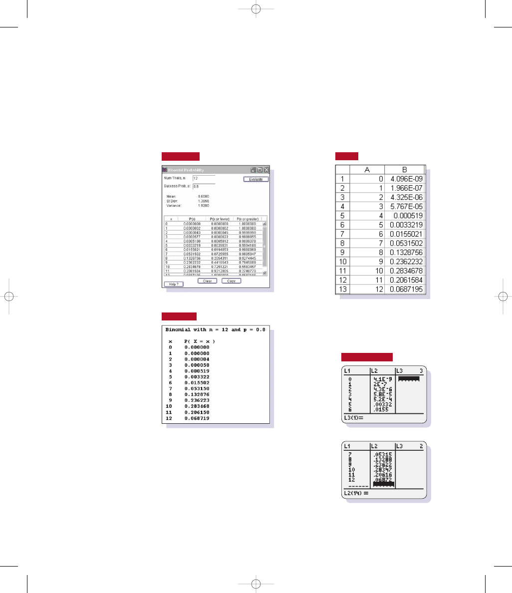
Method 3: Using Technology

STATDISK, Minitab, Excel, SPSS, SAS, and

the TI-83 84 Plus calculator are all examples of technologies that can be used to
find binomial probabilities. (Instead of directly providing probabilities for
individual values of x, SPSS and SAS are more difficult to use because they
provide cumulative probabilities of x or fewer successes.) Here are typical screen
displays that list binomial probabilities for n

12 and p 0.8.

STATDISK

Minitab

Excel

TI-83/84 Plus

5014_TriolaE/S_CH05pp198-243 12/7/05 2:57 PM Page 218

5-3

Binomial Probability Distributions

219

Given that we now have three different methods for finding binomial proba-

bilities, here is an effective and efficient strategy:

Use computer software or a TI-83 84 Plus calculator, if available.

If neither software nor the TI-83 84 Plus calculator is available, use Table A-1,
if possible.

If neither software nor the TI-83 84 Plus calculator is available and the
probabilities can’t be found using Table A-1, use the binomial probability
formula.

Rationale for the Binomial Probability Formula

The binomial probability formula is the basis for all three methods presented in
this section. Instead of accepting and using that formula blindly, let’s see why
it works.

Earlier in this section, we used the binomial probability formula for finding

the probability of getting exactly 7 Mexican-Americans when 12 jurors are ran-
domly selected from a population that is 80% Mexican-American. For each selec-
tion, the probability of getting a Mexican-American is 0.8. If we use the multipli-
cation rule from Section 4-4, we get the following result:

P(selecting 7 Mexican-Americans followed by 5 people

that are not Mexican-American)

0.8 ? 0.8 ? 0.8 ? 0.8 ? 0.8 ? 0.8 ? 0.8 ? 0.2 ? 0.2 ? 0.2 ? 0.2 ? 0.2
0.8

? 0.2

0.0000671

This result isn’t correct because it assumes that the first seven jurors are
Mexican-Americans and the last five are not, but there are other arrangements
possible for seven Mexican-Americans and five people that are not Mexican-
American.

In Section 4-7 we saw that with seven subjects identical to each other (such as

Mexican-Americans) and five other subjects identical to each other (such as non-
Mexican-Americans), the total number of arrangements (permutations) is 12!
[(7

5)!7!] or 792. Each of those 792 different arrangements has a probability of

0.8

? 0.2

, so the total probability is as follows:

P(7 Mexican-Americans among 12 jurors)

Generalize this result as follows: Replace 12 with n, replace 7 with x, replace 0.8
with p, replace 0.2 with q, and express the exponent of 5 as 12

7, which can be re-

placed with n

x. The result is the binomial probability formula. That is, the bino-

mial probability formula is a combination of the multiplication rule of probability

12!

s12 2 7d!7!

? 0.8

? 0.2

TriolaE/S_CH05pp198-243 11/11/05 7:33 AM Page 219

220

Chapter 5

Discrete Probability Distributions

Using Technology

Method 3 in this section involved the use of
STATDISK, Minitab, Excel, or a TI-83 84
Plus calculator. Screen displays shown with
Method 3 illustrated typical results obtained
by applying the following procedures for
finding binomial probabilities.

STATDISK

Select Analysis from the

main menu, then select the Binomial Prob-
abilities option. Enter the requested values
for n and p, and the entire probability distri-
bution will be displayed. Other columns
represent cumulative probabilities that are

obtained by adding the values of P(x) as you
go down or up the column.

MINITAB

First enter a column C1 of

the x values for which you want probabilities
(such as 0, 1, 2, 3, 4), then select Calc from
the main menu, and proceed to select the sub-
menu items of Probability Distributions
and Binomial. Select Probabilities, enter the
number of trials, the probability of success,
and C1 for the input column, then click OK.

EXCEL

List the values of x in column

A (such as 0, 1, 2, 3, 4). Click on cell B1,
then click on f

from the toolbar, and select

the function category Statistical and then the
function name BINOMDIST. In the dialog
box, enter A1 for the number of successes,
enter the number of trials, enter the probabil-
ity, and enter 0 for the binomial distribution
(instead of 1 for the cumulative binomial dis-
tribution). A value should appear in cell B1.
Click and drag the lower right corner of cell
B1 down the column to match the entries in
column A, then release the mouse button.

TI-83/84 PLUS

Press 2nd VARS (to

get DISTR, which denotes “distributions”),
then select the option identified as binompdf(.
Complete the entry of binompdf(n, p, x) with
specific values for n, p, and x, then press
ENTER, and the result will be the probability
of getting x successes among n trials.

You could also enter binompdf(n, p) to get a
list of all of the probabilities corresponding to
x

0, 1, 2, . . . , n. You could store this list in

L2 by pressing STO

➞ L2. You could then

enter the values of 0, 1, 2, . . . , n in list L1,
which would allow you to calculate statistics
(by entering STAT, CALC, then L1, L2) or
view the distribution in a table format (by
pressing STAT, then EDIT).

The command binomcdf yields cumulative
probabilities from a binomial distribution.
The command binomcdf(n, p, x) provides
the sum of all probabilities from x

through the specific value entered for x.

5-3

BASIC SKILLS AND CONCEPTS

Statistical Literacy and Critical Thinking

Notation

When using the binomial probability distribution for analyzing guesses on a

multiple-choice quiz, what is wrong with letting p denote the probability of getting a
correct answer while x counts the number of wrong answers?

Independence

Assume that we want to use the binomial probability distribution for

analyzing the genders when 12 jurors are randomly selected from a large population
of potential jurors. If selection is made without replacement, are the selections inde-
pendent? Can the selections be treated as being independent so that the binomial
probability distribution can be used?

Table A-1

Because the binomial probabilities in Table A-1 are so easy to find, why

don’t we use that table every time that we need to find a binomial probability?

and the counting rule for the number of arrangements of n items when x of them
are identical to each other and the other n

x are identical to each other. (See

Exercises 13 and 14.)

Psxd 5

sn 2 xd!x!

? p

? q

n2x

The number of outcomes with ex-
actly x successes among n trials

The probability of x successes among
n trials for any one particular order

TriolaE/S_CH05pp198-243 11/11/05 7:33 AM Page 220

5-3

Binomial Probability Distributions

221

Binomial Probabilities

When trying to find the probability of getting exactly two 6s

when a die is rolled five times, why can’t the answer be found as follows: Use the
multiplication rule to find the probability of getting two 6s followed by three out-
comes that are not 6, which is (1 6)(1 6)(5 6)(5 6)(5 6)?

Identifying Binomial Distributions. In Exercises 5–12, determine whether the given pro-
cedure results in a binomial distribution. For those that are not binomial, identify at least
one requirement that is not satisfied.

5. Randomly selecting 12 jurors and recording their nationalities

6. Surveying 12 jurors and recording whether there is a “no” response when they are

asked if they have ever been convicted of a felony

7. Treating 50 smokers with Nicorette and asking them how their mouth and throat feel

8. Treating 50 smokers with Nicorette and recording whether there is a “yes” response

when they are asked if they experience any mouth or throat soreness

9. Recording the genders of 250 newborn babies

10. Recording the number of children in 250 families

11. Surveying 250 married couples and recording whether there is a “yes” response when

they are asked if they have any children

12. Determining whether each of 500 defibrillators is acceptable or defective

13.

Finding Probabilities When Guessing Answers

Multiple-choice questions each have

five possible answers (a, b, c, d, e), one of which is correct. Assume that you guess the
answers to three such questions.
a. Use the multiplication rule to find the probability that the first two guesses are

wrong and the third is correct. That is, find P(WWC), where C denotes a correct
answer and W denotes a wrong answer.

b. Beginning with WWC, make a complete list of the different possible arrangements

of two wrong answers and one correct answer, then find the probability for each
entry in the list.

c. Based on the preceding results, what is the probability of getting exactly one cor-

rect answer when three guesses are made?

14.

Finding Probabilities When Guessing Answers

A test consists of multiple-choice

questions, each having four possible answers (a, b, c, d), one of which is correct. As-
sume that you guess the answers to six such questions.
a. Use the multiplication rule to find the probability that the first two guesses are

wrong and the last four guesses are correct. That is, find P(WWCCCC), where C
denotes a correct answer and W denotes a wrong answer.

b. Beginning with WWCCCC, make a complete list of the different possible arrange-

ments of two wrong answers and four correct answers, then find the probability for
each entry in the list.

c. Based on the preceding results, what is the probability of getting exactly four cor-

rect answers when six guesses are made?

Using Table A-1. In Exercises 15–20, assume that a procedure yields a binomial distri-
bution with a trial repeated n times. Use Table A-1 to find the probability of x successes
given the probability p of success on a given trial.

15. n

3, x 0, p 0.05

16. n

4, x 3, p 0.30

TriolaE/S_CH05pp198-243 11/11/05 7:34 AM Page 221

222

Chapter 5

Discrete Probability Distributions

17. n

8, x 4, p 0.05

18. n

8, x 7, p 0.20

19. n

14, x 2, p 0.30

20. n

15, x 12, p 0.90

Using the Binomial Probability Formula. In Exercises 21–24, assume that a procedure
yields a binomial distribution with a trial repeated n times. Use the binomial probability
formula to find the probability of x successes given the probability p of success on a sin-
gle trial.

21. n

5, x 2, p 0.25

22. n

6, x 4, p 0.75

23. n

9, x 3, p 1 4

24. n

10, x 2, p 2 3

Using Computer Results. In Exercises 25–28, refer to the Minitab display below. The
probabilities were obtained by entering the values of n

6 and p 0.167. In a clinical

test of the drug Lipitor, 16.7% of the subjects treated with 10 mg of atorvastatin experi-
enced headaches (based on data from Parke-Davis). In each case, assume that 6 subjects
are randomly selected and treated with 10 mg of atorvastatin, then find the indicated
probability.

Binomial with n = 6 and
p = 0.167000

P(X

0.00

0.3341

1.00

0.4019

2.00

0.2014

3.00

0.0538

4.00

0.0081

5.00

0.0006

6.00

0.0000

25. Find the probability that at least five of the subjects experience headaches. Is it un-

usual to have at least five of six subjects experience headaches?

26. Find the probability that at most two subjects experience headaches. Is it unusual to

have at most two of six subjects experience headaches?

27. Find the probability that more than one subject experiences headaches. Is it unusual to

have more than one of six subjects experience headaches?

28. Find the probability that at least one subject experiences headaches. Is it unusual to

have at least one of six subjects experience headaches?

29.

TV Viewer Surveys

The CBS television show 60 Minutes has been successful for

many years. That show recently had a share of 20, meaning that among the TV sets in
use, 20% were tuned to 60 Minutes (based on data from Nielsen Media Research). As-
sume that an advertiser wants to verify that 20% share value by conducting its own
survey, and a pilot survey begins with 10 households having TV sets in use at the time
of a 60 Minutes broadcast.
a. Find the probability that none of the households are tuned to 60 Minutes.
b. Find the probability that at least one household is tuned to 60 Minutes.

MINITAB

TriolaE/S_CH05pp198-243 11/11/05 7:34 AM Page 222

5-3

Binomial Probability Distributions

223

c. Find the probability that at most one household is tuned to 60 Minutes.
d. If at most one household is tuned to 60 Minutes, does it appear that the 20% share

value is wrong? Why or why not?

30.

IRS Audits

The Hemingway Financial Company prepares tax returns for individuals.

(Motto: “We also write great fiction.”) According to the Internal Revenue Service, in-
dividuals making $25,000

$50,000 are audited at a rate of 1%. The Hemingway

Company prepares five tax returns for individuals in that tax bracket, and three of
them are audited.
a. Find the probability that when 5 people making $25,000

$50,000 are randomly

selected, exactly 3 of them are audited.

b. Find the probability that at least 3 people are audited.
c. Based on the preceding results, what can you conclude about the Hemingway cus-

tomers? Are they just unlucky, or are they being targeted for audits?

31.

Acceptance Sampling

The Medassist Pharmaceutical Company receives large ship-

ments of aspirin tablets and uses this acceptance sampling plan: Randomly select and
test 24 tablets, then accept the whole batch if there is only one or none that doesn’t
meet the required specifications. If a particular shipment of thousands of aspirin
tablets actually has a 4% rate of defects, what is the probability that this whole ship-
ment will be accepted?

32.

Affirmative Action Programs

A study was conducted to determine whether there

were significant differences between medical students admitted through special pro-
grams (such as affirmative action) and medical students admitted through the regular
admissions criteria. It was found that the graduation rate was 94% for the medical stu-
dents admitted through special programs (based on data from the Journal of the
American Medical Association).
a. If 10 of the students from the special programs are randomly selected, find the

probability that at least 9 of them graduated.

b. Would it be unusual to randomly select 10 students from the special programs and

get only 7 that graduate? Why or why not?

33.

Overbooking Flights

Air America has a policy of booking as many as 15 persons on

an airplane that can seat only 14. (Past studies have revealed that only 85% of the
booked passengers actually arrive for the flight.) Find the probability that if Air
America books 15 persons, not enough seats will be available. Is this probability low
enough so that overbooking is not a real concern for passengers?

34.

Author’s Slot Machine

The author purchased a slot machine that is configured so that

there is a 1 2000 probability of winning the jackpot on any individual trial. Although
no one would seriously consider tricking the author, suppose that a guest claims that
she played the slot machine 5 times and hit the jackpot twice.
a. Find the probability of exactly two jackpots in 5 trials.
b. Find the probability of at least two jackpots in 5 trials.
c. Does the guest’s claim of two jackpots in 5 trials seem valid? Explain.

35.

Identifying Gender Discrimination

After being rejected for employment, Kim Kelly

learns that the Bellevue Credit Company has hired only two women among the last 20
new employees. She also learns that the pool of applicants is very large, with an ap-
proximately equal number of qualified men and women. Help her address the charge
of gender discrimination by finding the probability of getting two or fewer women
when 20 people are hired, assuming that there is no discrimination based on gender.
Does the resulting probability really support such a charge?

TriolaE/S_CH05pp198-243 11/11/05 7:34 AM Page 223

224

Chapter 5

Discrete Probability Distributions

36.

Improving Quality

The Write Right Company manufactures ballpoint pens and has

been experiencing a 5% rate of defective pens. Modifications are made to the manu-
facturing process in an attempt to improve quality, and the manager claims that the
modified procedure is better, because a test of 50 pens shows that only one is
defective.
a. Assuming that the 5% rate of defects has not changed, find the probability that

among 50 pens, exactly one is defective.

b. Assuming that the 5% rate of defects has not changed, find the probability that

among 50 pens, none are defective.

c. What probability value should be used for determining whether the modified pro-

cess results in a defect rate that is less than 5%?

d. What do you conclude about the effectiveness of the modified production process?

5-3

BEYOND THE BASICS

37.

Geometric Distribution

If a procedure meets all the conditions of a binomial distribu-

tion except that the number of trials is not fixed, then the geometric distribution can
be used. The probability of getting the first success on the xth trial is given by P(x)

p(1

where p is the probability of success on any one trial. Assume that the

probability of a defective computer component is 0.2. Find the probability that the
first defect is found in the seventh component tested.

38.

Hypergeometric Distribution

If we sample from a small finite population without re-

placement, the binomial distribution should not be used because the events are not in-
dependent. If sampling is done without replacement and the outcomes belong to one
of two types, we can use the hypergeometric distribution. If a population has A ob-
jects of one type, while the remaining B objects are of the other type, and if n objects
are sampled without replacement, then the probability of getting x objects of type A
and n

x objects of type B is

In Lotto 54, a bettor selects six numbers from 1 to 54 (without repetition), and a win-
ning six-number combination is later randomly selected. Find the probability of getting
a. all six winning numbers.
b. exactly five of the winning numbers.
c. exactly three of the winning numbers.
d. no winning numbers.

39.

Multinomial Distribution

The binomial distribution applies only to cases involving two

types of outcomes, whereas the multinomial distribution involves more than two cate-
gories. Suppose we have three types of mutually exclusive outcomes denoted by A, B,
and C. Let P(A)

, P(B)

, and P(C)

. In n independent trials, the probability

of x

outcomes of type A, x

outcomes of type B, and x

outcomes of type C is given by

A genetics experiment involves six mutually exclusive genotypes identified as A, B,
C, D, E, and F, and they are all equally likely. If 20 offspring are tested, find the prob-
ability of getting exactly five A’s, four B’s, three C’s, two D’s, three E’s, and three F’s
by expanding the above expression so that it applies to six types of outcomes instead
of only three.

!dsx

? p

Psxd 5

sA 2 xd!x!

sB 2 n 1 xd!sn 2 xd!

sA 1 Bd!

sA 1 B 2 nd!n!

TriolaE/S_CH05pp198-243 11/11/05 7:34 AM Page 224

5-4

Mean, Variance, and Standard Deviation for the Binomial Distribution

225

Mean, Variance, and Standard
Deviation for the Binomial

5-4

Distribution

Key Concept

Section 5-3 introduced the binomial probability distribution, and

in this section we consider important characteristics of a binomial distribution, in-
cluding center, variation, and distribution. That is, given a particular binomial
probability distribution, we will present methods for finding its mean, variance,
and standard deviation. As in earlier sections, the objective is not to simply find
those values, but to interpret them and understand them.

Section 5-2 included methods for finding the mean, variance, and standard devi-

ation from a discrete probability distribution. Because a binomial distribution is a
special type of probability distribution, we could use Formulas 5-1, 5-3, and 5-4
(from Section 5-2) for finding the mean, variance, and standard deviation, but those
formulas can be greatly simplified for binomial distributions, as shown below.

For Any Discrete Probability Distribution

For Binomial Distributions

Formula 5-1

Formula 5-6

Formula 5-3

Formula 5-7

Formula 5-4

Formula 5-8

As in earlier sections, finding values for and

is fine, but it is especially impor-

tant to interpret and understand those values, so the range rule of thumb can be
very helpful. Using the range rule of thumb, we can consider values to be unusual
if they fall outside of the limits obtained from the following:

maximum usual value:

minimum usual value:

EXAMPLE

Selecting Jurors

In Section 5-2 we included an example

illustrating calculations for

and . We used the example of the random

variable x representing the number of Mexican-Americans on a jury of 12
people. (We are assuming that the jurors are randomly selected from a
population that is 80% Mexican-American. See Table 5-3 on page 207 for the
calculations that illustrate Formulas 5-1 and 5-4.) Use Formulas 5-6 and 5-8
to find the mean and standard deviation for the numbers of Mexican-
Americans on juries selected from this population that is 80% Mexican-
American.

SOLUTION

Using the values n

12, p 0.8, and q 0.2, Formulas 5-6

and 5-8 can be applied as follows:

(rounded)

If you compare these calculations to the calculations in Table 5-3, it should be
obvious that Formulas 5-6 and 5-8 are substantially easier to use.

s 5 2npq 5 2s12ds0.8ds0.2d 5 1.4

m 5 np 5 s12ds0.8d 5 9.6

m 2 2s

m 1 2s

s 5 2npq

s 5 2S

? Psxd

4 2 m

5 npq

5 S

? Psxd

4 2 m

m 5 np

m 5 S

3x ? Psxd4

TriolaE/S_CH05pp198-243 11/11/05 7:34 AM Page 225

226

Chapter 5

Discrete Probability Distributions

Formula 5-6 for the mean makes sense intuitively. If 80% of a population is

Mexican-American and 12 people are randomly selected, we expect to get around
12 ? 0.8

9.6 Mexican-Americans, and this result can be easily generalized as

np. The variance and standard deviation are not so easily justified, and we

will omit the complicated algebraic manipulations that lead to Formulas 5-7 and
5-8. Instead, refer again to the preceding example and Table 5-3 to verify that for
a binomial distribution, Formulas 5-6, 5-7, and 5-8 will produce the same results
as Formulas 5-1, 5-3, and 5-4.

EXAMPLE

Grand Jury Selection

The Chapter Problem notes

that in Hidalgo County, Texas, 80% of those eligible for jury duty
were Mexican-Americans. It was also noted that during a period of 11

years, 870 people were selected for duty on a grand jury.

Assuming that groups of 870 grand jurors are randomly selected, find the
mean and standard deviation for the numbers of Mexican-Americans.

Use the range rule of thumb to find the minimum usual number and the
maximum usual number of Mexican-Americans. Based on those numbers,
can we conclude that the actual result of 339 Mexican-Americans is
unusual? Does this suggest that the selection process discriminated against
Mexican-Americans?

SOLUTION

Assuming that jurors were randomly selected, we have n

870 people se-

lected with p

0.80, and q 0.20. We can find the mean and standard de-

viation for the number of Mexican-Americans by using Formulas 5-6 and
5-8 as follows:

np (870)(0.80) 696.0

For groups of 870 randomly selected jurors, the mean number of Mexican-
Americans is 696.0 and the standard deviation is 11.8.

We must now interpret the results to determine whether 339 Mexican-
Americans is a result that could easily occur by chance, or whether that re-
sult is so unlikely that the selection process appears to be discriminatory.
We will use the range rule of thumb as follows:

maximum usual value:

696.0 2(11.8) 719.6

minimum usual value:

696.0 2(11.8) 672.4

INTERPRETATION

According to the range rule of thumb, values are consid-

ered to be usual if they are between 672.4 and 719.6, so 339 Mexican-
Americans is an unusual result because it is not between those two values. It is
very unlikely that we would get as few as 339 Mexican-Americans just by
chance. In fact, the Supreme Court ruled that the result of only 339 Mexican-

m 2 2s

m 1 2s

s 5 2npq 5 2s870ds0.80ds0.20d 5 11.8

5014_TriolaE/S_CH05pp198-243 11/23/05 8:50 AM Page 226

5-4

Mean, Variance, and Standard Deviation for the Binomial Distribution

227

Americans was significant evidence of a jury selection process that is biased.
The Castaneda v. Partida decision became an important judicial ruling, and it
was actually based on application of the binomial probability distribution.

Remember that finding values for the mean

and standard deviation

important, but it is particularly important to be able to interpret those values by
using such devices as the range rule of thumb for identifying a range of usual val-
ues.

5-4

BASIC SKILLS AND CONCEPTS

Statistical Literacy and Critical Thinking

Identifying Unusual Values

If we consider an experiment of generating 100 births and

recording the genders of the babies, the mean number of girls is 50 and the standard
deviation is 5 girls. Would it be unusual to get 70 girls in 100 births? Why or why not?

Identifying Unusual Values

A manufacturing process has a defect rate of 10%, mean-

ing that 10% of the items produced are defective. If batches of 80 items are produced,
the mean number of defects per batch is 8.0 and the standard deviation is 2.7. Would it
be unusual to get only five defects in a batch? Why or why not?

Variance

A researcher plans an experimental design in such a way that when ran-

domly selecting treatment groups of people, the mean number of females is 3.0 and
the standard deviation is 1.2 females. What is the variance? (Express the answer in-
cluding the appropriate units.)

Mean and Standard Deviation

A researcher conducts an observational study, then

uses the methods of this section to find that the mean is 5.0 while the standard devia-
tion is -2.0. What is wrong with these results?

Finding u, , and Unusual Values. In Exercises 5–8, assume that a procedure yields a
binomial distribution with n trials and the probability of success for one trial is p. Use the
given values of n and p to find the mean

and standard deviation

. Also, use the range

rule of thumb to find the minimum usual value

and the maximum usual value

5. n

200, p 0.4

6. n

60, p 0.25

7. n

1492, p 1 4

8. n

1068, p 2 3

Guessing Answers

Several psychology students are unprepared for a surprise true

false test with 16 questions, and all of their answers are guesses.
a. Find the mean and standard deviation for the number of correct answers for such

students.

b. Would it be unusual for a student to pass by guessing and getting at least 10 correct

answers? Why or why not?

10.

Guessing Answers

Several economics students are unprepared for a multiple-choice

quiz with 25 questions, and all of their answers are guesses. Each question has five
possible answers, and only one of them is correct.

m 1 2s

m 2 2s

continued

TriolaE/S_CH05pp198-243 11/11/05 7:34 AM Page 227

228

Chapter 5

Discrete Probability Distributions

a. Find the mean and standard deviation for the number of correct answers for such

students.

b. Would it be unusual for a student to pass by guessing and getting at least 15 correct

answers? Why or why not?

11.

Are 20% of M&M Candies Orange?

Mars, Inc., claims that 20% of its M&M plain

candies are orange, and a sample of 100 such candies is randomly selected.
a. Find the mean and standard deviation for the number of orange candies in such

groups of 100.

b. Data Set 13 in Appendix B consists of a random sample of 100 M&Ms in which 25

are orange. Is this result unusual? Does it seem that the claimed rate of 20% is
wrong?

12.

Are 14% of M&M Candies Yellow?

Mars, Inc., claims that 14% of its M&M plain

candies are yellow, and a sample of 100 such candies is randomly selected.
a. Find the mean and standard deviation for the number of yellow candies in such

groups of 100.

b. Data Set 13 in Appendix B consists of a random sample of 100 M&Ms in which 8

are yellow. Is this result unusual? Does it seem that the claimed rate of 14% is
wrong?

13.

Gender Selection

In a test of the MicroSort method of gender selection, 325 babies

are born to couples trying to have baby girls, and 295 of those babies are girls (based
on data from the Genetics & IVF Institute).
a. If the gender-selection method has no effect and boys and girls are equally likely,

find the mean and standard deviation for the numbers of girls born in groups of
325.

b. Is the result of 295 girls unusual? Does it suggest that the gender-selection method

appears to be effective?

14.

Gender Selection

In a test of the MicroSort method of gender selection, 51 babies are

born to couples trying to have baby boys, and 39 of those babies are boys (based on
data from the Genetics & IVF Institute).
a. If the gender-selection method has no effect and boys and girls are equally likely,

find the mean and standard deviation for the numbers of boys born in groups of 51.

b. Is the result of 39 boys unusual? Does it suggest that the gender-selection method

appears to be effective?

15.

Deciphering Messages

The Central Intelligence Agency has specialists who analyze

the frequencies of letters of the alphabet in an attempt to decipher intercepted mes-
sages. In standard English text, the letter r is used at a rate of 7.7%.
a. Find the mean and standard deviation for the number of times the letter r will be

found on a typical page of 2600 characters.

b. In an intercepted message sent to Iraq, a page of 2600 characters is found to have

the letter r occurring 175 times. Is this unusual?

16.

Mendelian Genetics

When Mendel conducted his famous genetics experiments with

peas, one sample of offspring consisted of 580 peas, and Mendel theorized that 25%
of them would be yellow peas.
a. If Mendel’s theory is correct, find the mean and standard deviation for the numbers

of yellow peas in such groups of 580 offspring peas.

b. The actual results consisted of 152 yellow peas. Is that result unusual? What does

this result suggest about Mendel’s theory?

TriolaE/S_CH05pp198-243 11/11/05 7:34 AM Page 228

5-4

Mean, Variance, and Standard Deviation for the Binomial Distribution

229

17.

Voting

In a past presidential election, the actual voter turnout was 61%. In a survey,

1002 subjects were asked if they voted in the presidential election.
a. Find the mean and standard deviation for the numbers of actual voters in groups of

1002.

b. In the survey of 1002 people, 701 said that they voted in the last presidential elec-

tion (based on data from ICR Research Group). Is this result consistent with the ac-
tual voter turnout, or is this result unlikely to occur with an actual voter turnout of
61%? Why or why not?

c. Based on these results, does it appear that accurate voting results can be obtained

by asking voters how they acted?

18.

Cell Phones and Brain Cancer

In a study of 420,095 cell phone users in Denmark, it

was found that 135 developed cancer of the brain or nervous system. If we assume
that such cancer is not affected by cell phones, the probability of a person having such
a cancer is 0.000340.
a. Assuming that cell phones have no effect on cancer, find the mean and standard

deviation for the numbers of people in groups of 420,095 that can be expected to
have cancer of the brain or nervous system.

b. Based on the results from part (a), is it unusual to find that among 420,095 peo-

ple, there are 135 cases of cancer of the brain or nervous system? Why or why
not?

c. What do these results suggest about the publicized concern that cell phones are a

health danger because they increase the risk of cancer of the brain or nervous
system?

19.

Cholesterol Drug

In a clinical trial of Lipitor (atorvastatin), a common drug used to

lower cholesterol, 863 patients were given a treatment of 10-mg atorvastatin tablets.
That group consists of 19 patients who experienced flu symptoms (based on data from
Pfizer, Inc.). The probability of flu symptoms for a person not receiving any treatment
is 0.019.
a. Assuming that Lipitor has no effect on flu symptoms, find the mean and standard

deviation for the numbers of people in groups of 863 that can be expected to have
flu symptoms.

b. Based on the result from part (a), is it unusual to find that among 863 people, there

are 19 who experience flu symptoms? Why or why not?

c. Based on the preceding results, do flu symptoms appear to be an adverse reaction

that should be of concern to those who use Lipitor?

20.

Test of Touch Therapy

Nine-year-old Emily Rosa conducted this test: A professional

touch therapist put both hands through a cardboard partition and Emily would use a
coin toss to randomly select one of the hands. Emily would place her hand just above
the hand of the therapist, who was then asked to identify the hand that Emily had se-
lected. The touch therapists believed that they could sense the energy field and iden-
tify the hand that Emily had selected. The trial was repeated 280 times. (Based on
data from “A Close Look at Therapeutic Touch,” by Rosa et al., Journal of the Ameri-
can Medical Association,Vol. 279, No. 13.)
a. Assuming that the touch therapists have no special powers and made random

guesses, find the mean and standard deviation for the numbers of correct responses
in groups of 280 trials.

b. The professional touch therapists identified the correct hand 123 times in the 280

trials. Is that result unusual? What does the result suggest about the ability of touch
therapists to select the correct hand by sensing an energy field?

TriolaE/S_CH05pp198-243 11/11/05 7:34 AM Page 229

230

Chapter 5

Discrete Probability Distributions

5-4

BEYOND THE BASICS

21.

Using the Empirical Rule

An experiment is designed to test the effectiveness of the

MicroSort method of gender selection, and 100 couples try to have baby girls using
the MicroSort method. Assume that boys and girls are equally likely and also assume
that the method of gender selection has no effect.
a. Using the methods of this section, what are the minimum and maximum usual

numbers of girls in groups of 100 randomly selected babies?

b. The empirical rule (see Section 3-3) applies to distributions that are bell-shaped. Is

the binomial probability distribution for this experiment (approximately) bell-
shaped? How do you know?

c. Assuming that the distribution is bell-shaped, how likely is it that the number of

girls will fall between 40 and 60 (according to the empirical rule)?

22.

Acceptable Defective Products

Mario’s Pizza Parlor has just opened. Due to a lack

of employee training, there is only a 0.8 probability that a pizza will be edible. An or-
der for five pizzas has just been placed. What is the minimum number of pizzas that
must be made in order to be at least 99% sure that there will be five that are edible?

5-5

Poisson Probability Distributions

Key Concept

This section introduces the Poisson distribution, which is an im-

portant discrete probability distribution. It is important because it is often used for
describing the behavior of rare events (with small probabilities). We should know
the requirements for using the Poisson distribution, and we should know how to
calculate probabilities using Formula 5-9. We should also know that when the
Poisson distribution applies to a variable with mean , the standard deviation is

.
The Poisson distribution is used for describing behavior such as radioactive

decay, arrivals of people in a line, eagles nesting in a region, patients arriving at an
emergency room, and Internet users logging onto a Web site. For example, sup-
pose your local hospital experiences a mean of 2.3 patients arriving at the emer-
gency room on Fridays between 10:00

. and 11:00

. We can find the proba-

bility that for a randomly selected Friday between 10:00

. and 11:00

exactly four patients arrive. We use the Poisson distribution, defined as follows.

Definition

The Poisson distribution is a discrete probability distribution that applies to
occurrences of some event over a specified interval. The random variable x is
the number of occurrences of the event in an interval. The interval can be
time, distance, area, volume, or some similar unit. The probability of the
event occurring x times over an interval is given by Formula 5-9.

Formula 5-9

where e

2.71828

Psxd 5

? e

TriolaE/S_CH05pp198-243 11/11/05 7:34 AM Page 230

5-5

Poisson Probability Distributions

231

Requirements for the Poisson Distribution

●

The random variable x is the number of occurrences of an event over some
interval.

●

The occurrences must be random.

●

The occurrences must be independent of each other.

●

The occurrences must be uniformly distributed over the interval being used.

Parameters of the Poisson Distribution

●

The mean is

●

The standard deviation is s 5

!m.

Queues

Queuing theory is a branch of

mathematics that uses proba-

bility and statistics. The study

of queues, or waiting lines, is

important to businesses such

as supermarkets, banks, fast-

food restaurants, airlines, and

amusement parks. Grand

Union supermarkets try to

keep checkout lines no longer

than three shoppers. Wendy’s

introduced the “Express Pak”

to expedite servicing its nu-

merous drive-through cus-

tomers. Disney conducts ex-

tensive studies of lines at its

amusement parks so that it

can keep patrons happy and

plan for expansion. Bell Lab-

oratories uses queuing theory

to optimize telephone net-

work usage, and factories use

it to design efficient produc-

tion lines.

A Poisson distribution differs from a binomial distribution in these fundamen-

tal ways:

The binomial distribution is affected by the sample size n and the probability
p, whereas the Poisson distribution is affected only by the mean

In a binomial distribution, the possible values of the random variable x are 0,
1, . . . , n, but a Poisson distribution has possible x values of 0, 1, 2, . . . , with
no upper limit.

EXAMPLE

World War II Bombs

In analyzing hits by V-1 buzz bombs

in World War II, South London was subdivided into 576 regions, each with an
area of 0.25 km

. A total of 535 bombs hit the combined area of 576 regions.

If a region is randomly selected, find the probability that it was hit exactly
twice.

Based on the probability found in part (a), how many of the 576 regions are
expected to be hit exactly twice?

SOLUTION

The Poisson distribution applies because we are dealing with the occur-
rences of an event (bomb hits) over some interval (a region with area of
0.25 km

). The mean number of hits per region is

Because we want the probability of exactly two hits in a region, we let x

2 and use Formula 5-9 as follows:

The probability of a particular region being hit exactly twice is P(2)

0.170.

continued

Psxd 5

? e

0.929

? 2.71828

20.929

0.863 ? 0.395

5 0.170

m 5

number of bomb hits

number of regions

535

576

5 0.929

TriolaE/S_CH05pp198-243 11/11/05 7:34 AM Page 231

232

Chapter 5

Discrete Probability Distributions

Because there is a probability of 0.170 that a region is hit exactly twice, we
expect that among the 576 regions, the number that is hit exactly twice is
576 ? 0.170

97.9.

In the preceding example, we can also calculate the probabilities and expected

values for 0, 1, 3, 4, and 5 hits. (We stop at x

5 because no region was hit more

than five times, and the probabilities for x

5 are 0.000 when rounded to three

decimal places.) Those probabilities and expected values are listed in Table 5-5.
The fourth column of Table 5-5 describes the results that actually occurred during
World War II. There were 229 regions that had no hits, 211 regions that were hit
once, and so on. We can now compare the frequencies predicted with the Poisson
distribution (third column) to the actual frequencies (fourth column) to conclude
that there is very good agreement. In this case, the Poisson distribution does a
good job of predicting the results that actually occurred. (Section 11-2 describes a
statistical procedure for determining whether such expected frequencies constitute
a good “fit” to the actual frequencies. That procedure does suggest that there is a
good fit in this case.)

Poisson as Approximation to Binomial

The Poisson distribution is sometimes used to approximate the binomial distribu-
tion when n is large and p is small. One rule of thumb is to use such an approxi-
mation when the following two conditions are both satisfied.

Requirements for Using the Poisson Distribution as an
Approximation to the Binomial

100

If both of these conditions are satisfied and we want to use the Poisson distribu-
tion as an approximation to the binomial distribution, we need a value for

and

that value can be calculated by using Formula 5-6 (first presented in Section 5-4):

Formula 5-6

m 5 np

Table 5-5

V-1 Buzz Bomb Hits for 576 Regions in South London

Number

Expected Number

Actual Number

of Bomb Hits

Probability

of Regions

0.395

227.5

229

0.367

211.4

211

0.170

97.9

0.053

30.5

0.012

6.9

0.002

1.2

TriolaE/S_CH05pp198-243 11/11/05 7:34 AM Page 232

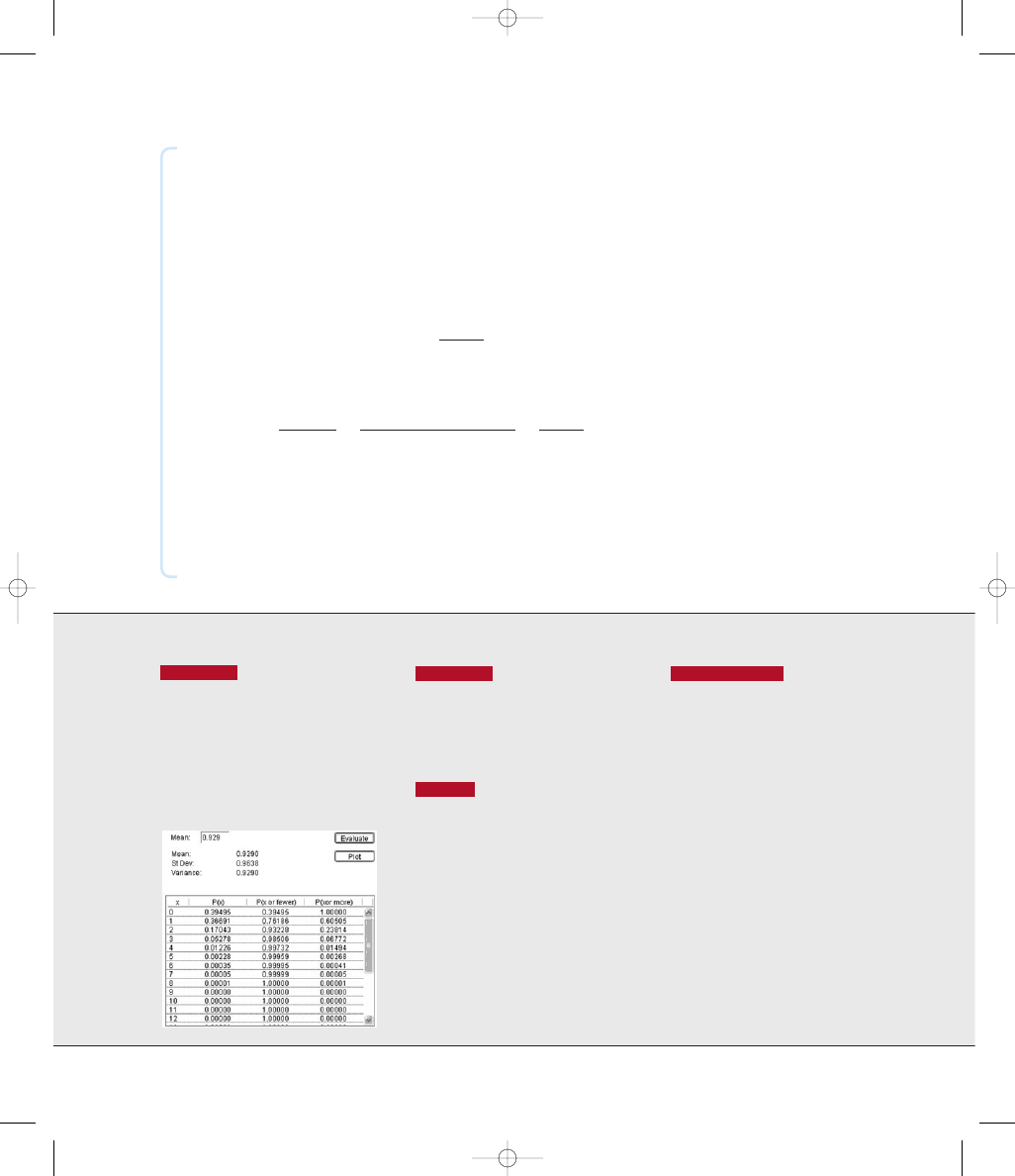
5-5

Poisson Probability Distributions

233

Using Technology

STATDISK

Select Analysis from the

main menu bar, then select Poisson Proba-
bilities and proceed to enter the value of the
mean . Click the Evaluate button and
scroll for values that do not fit in the initial
window. See the accompanying Statdisk dis-
play using the mean of 0.929 from the first
example in this section.

MINITAB

First enter the desired

value of x in column C1. Now select Calc
from the main menu bar, then select Proba-
bility Distributions, then Poisson. Enter
the value of the mean

and enter C1 for the

input column.

EXCEL

Click on fx on the main menu

bar, then select the function category of
Statistical, then select POISSON, then
click OK. In the dialog box, enter the values
for x and the mean, and enter 0 for “Cumula-
tive.” (Entering 1 for “Cumulative” results
in the probability for values up to and in-
cluding the entered value of x.)

TI-83/84 PLUS

Press 2nd VARS (to

get DISTR), then select option B:
poissonpdf(. Now press ENTER, then pro-
ceed to enter , x (including the comma).
For , enter the value of the mean; for x, en-
ter the desired number of occurrences.

EXAMPLE

Kentucky Pick 4

In Kentucky’s Pick 4 game, you pay $1 to

select a sequence of four digits, such as 2283. If you play this game once every
day, find the probability of winning exactly once in 365 days.

SOLUTION

Because the time interval is 365 days, n

365. Because there is

one winning set of numbers among the 10,000 that are possible (from 0000 to
9999), p

1 10,000. The conditions n 100 and np 10 are both satisfied,

so we can use the Poisson distribution as an approximation to the binomial dis-
tribution. We first need the value of

which is found as follows:

Having found the value of

we can now find P(1):

Using the Poisson distribution as an approximation to the binomial distribu-
tion, we find that there is a 0.0352 probability of winning exactly once in 365
days. If we use the binomial distribution, we again get 0.0352, so we can see
that the Poisson approximation is quite good here. (Carrying more decimal
places would show that the Poisson approximation yields 0.03519177 and the
more accurate binomial result is 0.03519523.)

Ps1d 5

? e

0.0365

? 2.71828

20.0365

0.0352

5 0.0352

m 5 np 5 365 ?

10,000

5 0.0365

STATDISK

5014_TriolaE/S_CH05pp198-243 12/7/05 11:10 AM Page 233

234

Chapter 5

Discrete Probability Distributions

5-5

BASIC SKILLS AND CONCEPTS

Statistical Literacy and Critical Thinking

Poisson Distribution

What are the conditions for using the Poisson distribution?

Poisson Distribution

The random variable x represents the number of phone calls re-

ceived in an hour, and it has a Poisson distribution with a mean of 9. What is its stan-
dard deviation? What is its variance?

Parameters

When attempting to apply the Poisson distribution, which of the

following must be known: mean, standard deviation, variance, shape of the
distribution?

Poisson Binomial

An experiment involves rolling a die 6 times and counting the

number of 2s that occur. If we calculate the probability of x

0 occurrences of 2

using the Poisson distribution, we get 0.368, but we get 0.335 if we use the binomial
distribution. Which is the correct probability of getting no 2s when a die is rolled
6 times? Why is the other probability wrong?

Using a Poisson Distribution to Find Probability. In Exercises 5–8, assume that the
Poisson distribution applies and proceed to use the given mean to find the indicated
probability.

5. If

5, find P(4).

6. If

3 4, find P(2).

7. If

0.5, find P(3).

8. If

3.25, find P(5).

In Exercises 9–16, use the Poisson distribution to find the indicated probabilities.

Dandelions

Dandelions are studied for their effects on crop production and lawn

growth. In one region, the mean number of dandelions per square meter was found to
be 7.0 (based on data from Manitoba Agriculture and Food).
a. Find the probability of no dandelions in an area of 1 m

b. Find the probability of at least one dandelion in an area of 1 m

c. Find the probability of at most two dandelions in an area of 1 m

10.

Phone Calls

The author found that in one month (30 days), he made 47 cell phone

calls, which were distributed as follows: No calls were made on 17 days, 1 call was
made on each of 7 days, 3 calls were made on each of two days, 4 calls were made on
each of two days, 12 calls were made on one day, and 14 calls were made on one day.
a. Find the mean number of calls per day.
b. Use the Poisson distribution to find the probability of no calls on a day, and com-

pare the result to the actual relative frequency for the number of days with no calls.

c. Use the Poisson distribution to find the probability of one call on a day, and com-

pare the result to the actual relative frequency for the number of days with one
call.

d. Based on the preceding results, does it appear that the author’s cell phone calls

made in a day fit the Poisson distribution reasonably well? Why or why not?

11.

Radioactive Decay

Radioactive atoms are unstable because they have too much en-

ergy. When they release their extra energy, they are said to decay. When studying
cesium-137, it is found that during the course of decay over 365 days, 1,000,000
radioactive atoms are reduced to 977,287 radioactive atoms.
a. Find the mean number of radioactive atoms lost through decay in a day.
b. Find the probability that on a given day, 50 radioactive atoms decayed.

TriolaE/S_CH05pp198-243 11/11/05 7:34 AM Page 234

5-5

Poisson Probability Distributions

235

12.

Deaths from Horse Kicks

A classical example of the Poisson distribution involves

the number of deaths caused by horse kicks to men in the Prussian Army between
1875 and 1894. Data for 14 corps were combined for the 20-year period, and the 280
corps-years included a total of 196 deaths. After finding the mean number of deaths
per corps-year, find the probability that a randomly selected corps-year has the fol-
lowing numbers of deaths.

a. 0

b. 1

c. 2

d. 3

e. 4

The actual results consisted of these frequencies: 0 deaths (in 144 corps-years);
1 death (in 91 corps-years); 2 deaths (in 32 corps-years); 3 deaths (in 11 corps-years);
4 deaths (in 2 corps-years). Compare the actual results to those expected from the
Poisson probabilities. Does the Poisson distribution serve as a good device for pre-
dicting the actual results?

13.

Homicide Deaths

In one year, there were 116 homicide deaths in Richmond, Virginia

(based on “A Classroom Note on the Poisson Distribution: A Model for Homicidal
Deaths in Richmond, Va for 1991,” by Winston A. Richards in Mathematics and
Computer Education). For a randomly selected day, find the probability that the num-
ber of homicide deaths is

a. 0

b. 1

c. 2

d. 3

e. 4

Compare the calculated probabilities to these actual results: 268 days (no homicides);
79 days (1 homicide); 17 days (2 homicides); 1 day (3 homicides); no days with more
than 3 homicides.

14.

Earthquakes

For a recent period of 100 years, there were 93 major earthquakes (at

least 6.0 on the Richter scale) in the world (based on data from the World Almanac
and Book of Facts). Assuming that the Poisson distribution is a suitable model, find
the mean number of major earthquakes per year, then find the probability that the
number of earthquakes in a randomly selected year is

a. 0

b. 1

c. 2

d. 3

e. 4

f. 5

g. 6

h. 7

Here are the actual results: 47 years (0 major earthquakes); 31 years (1 major earth-
quake); 13 years (2 major earthquakes); 5 years (3 major earthquakes); 2 years (4 ma-
jor earthquakes); 0 years (5 major earthquakes); 1 year (6 major earthquakes); 1 year
(7 major earthquakes). After comparing the calculated probabilities to the actual re-
sults, is the Poisson distribution a good model?

5-5

BEYOND THE BASICS

15.

Poisson Approximation to Binomial

The Poisson distribution can be used to approxi-

mate a binomial distribution if n

100 and np 10. Assume that we have a binomial

distribution with n

100 and p 0.1. It is impossible to get 101 successes in such a

binomial distribution, but we can compute the probability that x

101 with the Pois-

son approximation. Find that value. How does the result agree with the impossibility
of having x

101 with a binomial distribution?

16.

Poisson Approximation to Binomial

For a binomial distribution with n

10 and p

0.5, we should not use the Poisson approximation because the conditions n

100 and

10 are not both satisfied. Suppose we go way out on a limb and use the Poisson

approximation anyway. Are the resulting probabilities unacceptable approximations?
Why or why not?

TriolaE/S_CH05pp198-243 11/11/05 7:34 AM Page 235

236

Chapter 5

Discrete Probability Distributions

Review

The concept of a probability distribution is a key element of statistics. A probabil-
ity distribution describes the probability for each value of a random variable. This
chapter includes only discrete probability distributions, but the following chapters
will include continuous probability distributions. The following key points were
discussed:

●

A random variable has values that are determined by chance.

●

A probability distribution consists of all values of a random variable, along
with their corresponding probabilities. A probability distribution must sat-
isfy two requirements:

and, for each value of x, 0

P(x) 1.

●

Important characteristics of a probability distribution can be explored by
constructing a probability histogram and by computing its mean and stan-
dard deviation using these formulas:

●

In a binomial distribution, there are two categories of outcomes and a fixed
number of independent trials with a constant probability. The probability of
x successes among n trials can be found by using the binomial probability
formula, or Table A-1, or software (such as STATDISK, Minitab, or Excel),
or a TI-83 84 Plus calculator.

●

In a binomial distribution, the mean and standard deviation can be easily
found by calculating the values of

np and .

●

A Poisson probability distribution applies to occurrences of some event over
a specific interval, and its probabilities can be computed with Formula 5-9.

●

Unusual outcomes: This chapter stressed the importance of interpreting re-
sults by distinguishing between outcomes that are usual and those that are
unusual. We used two different criteria: the range rule of thumb and the use
of probabilities.

Using the range rule of thumb to identify unusual values:

maximum usual value

minimum usual value

Using probabilities to identify unusual values:

●

Unusually high number of successes: x successes among n trials is an
unusually high number of successes if P(x or more)

0.05.*

●

Unusually low number of successes: x successes among n trials is an
unusually low number of successes if P(x or fewer)

0.05.*

m 2 2s

m 1 2s

s 5

!npq

s 5 2S

? Psxd

4 2 m

m 5 S

3x ? Psxd4

SPsxd 5 1

TriolaE/S_CH05pp198-243 11/11/05 7:34 AM Page 236

Review Exercises

237

Statistical Literacy and Critical Thinking

Probability Distribution

What is a probability distribution?

Probability Distribution

What are the requirements of a probability distribution?

Discrete Probability Distribution

The probability distributions described in this chap-

ter are discrete. What makes them discrete? What other type of probability distribu-
tion is there?

Probability Distributions

This chapter described the concept of a discrete probability

distribution, and then described the binomial and Poisson probability distributions.
Are all discrete probability distributions either binomial or Poisson? Why or why not?

Review Exercises

Multiple-Choice Test

Because they are so easy to correct, multiple-choice questions

are commonly used for class tests, SAT tests, MCAT tests for medical schools, and
many other circumstances. The table in the margin describes the probability distribu-
tion for the number of correct responses when someone makes random guesses for
10 multiple-choice questions on an SAT test. Each question has 5 possible answers (a,
b, c, d, e), one of which is correct. Assume that random guesses are made for each of
the 10 questions.

a. Verify that the table satisfies the requirements necessary for a probability distribution.

b. Find the mean number of correct responses.

c. Find the standard deviation for the numbers of correct responses when random

guesses are made for the 10 questions by many different subjects.

d. What is the probability that someone gets at least half of the questions correct?

e. When someone makes guesses for all 10 answers, what is the expected number of

correct answers?

f. What is the probability of getting at least 1 answer correct?

g. If someone gets at least 1 answer correct, does that mean that this person knows

something about the subject matter being tested?

TV Ratings

The television show Cold Case has a 15 share, meaning that while it is be-

ing broadcast, 15% of the TV sets in use are tuned to Cold Case (based on data from
Nielsen Media Research). A special focus group consists of 12 randomly selected
households (each with one TV set in use during the time of a Cold Case broadcast).

a. What is the expected number of sets tuned to Cold Case?

b. In such groups of 12, what is the mean number of sets tuned to Cold Case?

c. In such groups of 12, what is the standard deviation for the number of sets tuned to

Cold Case?

d. For such a group of 12, find the probability that exactly 3 TV sets are tuned to Cold

Case.

e. For such a group of 12, would it be unusual to find that no sets are tuned to Cold

Case? Why or why not?

P(x)

0.107

0.268

0.302

0.201

0.088

0.026

0.006

0.001

5014_TriolaE/S_CH05pp198-243 1/18/07 4:18 PM Page 237

238

Chapter 5

Discrete Probability Distributions

Reasons for Being Fired

“Inability to get along with others” is the reason cited in 17%

of worker firings (based on data from Robert Half International, Inc.). Concerned about
her company’s working conditions, the personnel manager at the Boston Finance Com-
pany plans to investigate the five employee firings that occurred over the past year.

a. Assuming that the 17% rate applies, find the probability that among those five employ-

ees, the number fired because of an inability to get along with others is at least four.

b. If the personnel manager actually does find that at least four of the firings are due

to an inability to get along with others, does this company appear to be very differ-
ent from other typical companies? Why or why not?

Deaths

Currently, an average of 7 residents of the village of Westport (population

760) die each year (based on data from the National Center for Health Statistics).

a. Find the mean number of deaths per day.

b. Find the probability that on a given day, there are no deaths.

c. Find the probability that on a given day, there is one death.

d. Find the probability that on a given day, there is more than one death.

e. Based on the preceding results, should Westport have a contingency plan to handle

more than one death per day? Why or why not?

Cumulative Review Exercises

Weights: Analysis of Last Digits

The accompanying table lists the last digits of

weights of the subjects listed in Data Set 1 in Appendix B. The last digits of a data set
can sometimes be used to determine whether the data have been measured or simply
reported. The presence of disproportionately more 0s and 5s is often a sure indicator
that the data have been reported instead of measured.

a. Find the mean and standard deviation of those last digits.

b. Construct the relative frequency table that corresponds to the given frequency table.

c. Construct a table for the probability distribution of randomly selected digits that

are all equally likely. List the values of the random variable x (0, 1, 2, . . . , 9) along
with their corresponding probabilities (0.1, 0.1, 0.1, . . . , 0.1), then find the mean
and standard deviation of this probability distribution.

d. Recognizing that sample data naturally deviate from the results we theoretically

expect, does it seem that the given last digits roughly agree with the distribution
we expect with random selection? Or does it seem that there is something about
the sample data (such as disproportionately more 0s and 5s) suggesting that the
given last digits are not random? (In Chapter 11, we will present a method for an-
swering such questions much more objectively.)

Determining the Effectiveness of an HIV Training Program

The New York State

Health Department reports a 10% rate of the HIV virus for the “at-risk” population. In
one region, an intensive education program is used in an attempt to lower that 10% rate.
After running the program, a follow-up study of 150 at-risk individuals is conducted.

a. Assuming that the program has no effect, find the mean and standard deviation for

the number of HIV cases in groups of 150 at-risk people.

TriolaE/S_CH05pp198-243 11/11/05 7:34 AM Page 238

Cumulative Review Exercises

239

b. Among the 150 people in the follow-up study, 8% (or 12 people) tested positive for

the HIV virus. If the program has no effect, is that rate unusually low? Does this
result suggest that the program is effective?

Credit Card Usage

A student of the author conducted a survey of credit card usage by

25 of her friends. Each subject was asked how many times he or she used a credit card
within the past seven days, and the results are listed as relative frequencies in the ac-
companying table.

a. Does the table constitute a probability distribution? Why or why not?

b. Assuming that the table does describe a probability distribution, what is the popula-

tion that it represents? Is it the population of all credit card holders in the United
States?

c. Does the type of sampling limit the usefulness of the data?

d. Find the mean number of credit card uses in the past seven days.

e. Find the standard deviation by assuming that the table is a relative frequency table

summarizing results from a sample of 25 subjects.

Relative Frequency

0.16

0.24

0.40

0.16

0.04

TriolaE/S_CH05pp198-243 11/11/05 7:34 AM Page 239

240

Chapter 5

Discrete Probability Distributions

Cooperative Group Activities

In-class activity

Win $1,000,000! The James Randi Ed-

ucational Foundation offers a $1,000,000 prize to anyone
who can show, “under proper observing conditions, evi-
dence of any paranormal, supernatural, or occult power
or event.” Divide into groups of three. Select one person
who will be tested for extrasensory perception (ESP) by
trying to correctly identify a digit randomly selected by
another member of the group. Another group member
should record the randomly selected digit, the digit
guessed by the subject, and whether the guess was cor-
rect or wrong. Construct the table for the probability dis-
tribution of randomly generated digits, construct the rela-
tive frequency table for the random digits that were
actually obtained, and construct a relative frequency
table for the guesses that were made. After comparing
the three tables, what do you conclude? What proportion
of guesses are correct? Does it seem that the subject has
the ability to select the correct digit significantly more
often than would be expected by chance?

In-class activity

See the preceding activity and design an

experiment that would be effective in testing someone’s
claim that they have the ability to identify the color of a
card selected from a standard deck of playing cards. De-
scribe the experiment with great detail. Because the prize
of $1,000,000 is at stake, we want to be careful to avoid
the serious mistake of concluding that the person has the
paranormal power when that power is not actually pre-

sent. There will likely be some chance that the subject
could make random guesses and be correct every time, so
identify a probability that is reasonable for the event of
the subject passing the test with random guesses. Be sure
that the test is designed so that this probability is equal to
or less than the probability value selected.

In-class activity

Suppose we want to identify the prob-

ability distribution for the number of children born to
randomly selected couples. For each student in the
class, find the number of brothers and sisters and record
the total number of children (including the student) in
each family. Construct the relative frequency table for
the result obtained. (The values of the random variable
x will be 1, 2, 3, . . .) What is wrong with using this rel-
ative frequency table as an estimate of the probability
distribution for the number of children born to ran-
domly selected couples?

Out-of-class activity

See Cumulative Review Exer-

cise 1, which suggests that an analysis of the last digits
of data can sometimes reveal whether the data have
been collected through actual measurements or re-
ported by the subjects. Refer to an almanac or the Inter-
net and find a collection of data (such as lengths of
rivers in the world), then analyze the distribution of last
digits to determine whether the values were obtained
through actual measurements.

TriolaE/S_CH05pp198-243 11/11/05 7:34 AM Page 240

From Data to Decision

241

Technology Project

American Airlines Flight 179 from New York to San Fran-
cisco uses a Boeing 767-300 with 213 seats. Because some
people with reservations don’t show up, American Airlines
can overbook by accepting more than 213 reservations. If
the flight is not overbooked, the airline will lose revenue
due to empty seats, but if too many seats are sold and some
passengers are denied seats, the airline loses money from
the compensation that must be given to the bumped passen-
gers. Assume that there is a 0.0995 probability that a pas-
senger with a reservation will not show up for the flight
(based on data from the IBM research paper “Passenger-
Based Predictive Modeling of Airline No-Show Rates” by
Lawrence, Hong, and Cherrier). Also assume that the airline
accepts 236 reservations for the 213 seats that are available.

Find the probability that when 236 reservations are accepted
for Flight 179, there are more passengers showing up than

there are seats available. That is, find the probability of
more than 213 people showing up with reservations, assum-
ing that 236 reservations were accepted. Because of the val-
ues involved, Table A-1 cannot be used, and calculations
with the binomial probability formula would be extremely
time-consuming and painfully tedious. The best approach is
to use statistics software or a TI-83 84 Plus calculator. See
Section 5-3 for instructions describing the use of STAT-
DISK, Minitab, Excel, or a TI-83 84 Plus calculator. Is the
probability of overbooking small enough so that it does not
happen very often, or does it seem too high so that changes
must be made to make it lower? Now use trial and error to
find the maximum number of reservations that could be ac-
cepted so that the probability of having more passengers
than seats is 0.05 or less.

From Data to Decision

Critical Thinking: Determining
criteria for concluding that a
gender-selection method
is effective

You are responsible for analyzing results
from a clinical trial of the effectiveness of a
new method of gender selection. Assume
that the sample size of n

50 couples has

already been established, and each couple
will have one child. Further assume that
each of the couples will be subjected to a

treatment that supposedly increases the like-
lihood that the child will be a girl.

There is a danger in obtaining results first,
then making conclusions about the results. If
the results are close to showing the effec-
tiveness of a treatment, it might be tempting
to conclude that there is an effect when, in
reality, there is no effect. It is better to estab-
lish criteria before obtaining results. Using
the methods of this chapter, identify the cri-
teria that should be used for concluding that
the treatment is effective in increasing the
likelihood of a girl. Among the 50 births,

how many girls would you require in order
to conclude that the gender-selection proce-
dure is effective? Explain how you arrived
at this result.

5014_TriolaE/S_CH05pp198-243 11/23/05 8:51 AM Page 241

242

Chapter 5

Discrete Probability Distributions

Probability Distributions
and Simulation

Probability distributions are used to predict the

outcome of the events they model. For example,

if we toss a fair coin, the distribution for the

outcome is a probability of 0.5 for heads and

0.5 for tails. If we toss the coin ten consecutive

times, we expect five heads and five tails. We

might not get this exact result, but in the long

run, over hundreds or thousands of tosses, we

expect the split between heads and tails to be

very close to “50–50”. Go to the Web site for

this textbook:

http://www.aw.com/triola

Proceed to the Internet Project for Chapter 5

where you will find two explorations. In the

first exploration you are asked to develop a

probability distribution for a simple experiment,

and use that distribution to predict the outcome

of repeated trial runs of the experiment. In the

second exploration, we will analyze a more

complicated situation: the paths of rolling

marbles as they move in pinball-like fashion

through a set of obstacles. In each case, a

dynamic visual simulation will allow you to

compare the predicted results with a set of

experimental outcomes.

Internet Project

5014_TriolaE/S_CH05pp198-243 11/23/05 8:51 AM Page 242

Statistics @ Work

243

Statistics @ Work

What do you do?

We do public polling. We survey public
issues, approval ratings of public officials
in New York city, New York State, and
nationwide. We don’t do partisan pol-
ling for political parties, political candi-
dates, or lobby groups. We are indepen-
dently funded by Marist College and we
have no outside funding that in any way
might suggest that we are doing re-
search for any particular group on any
one issue.

How do you select survey
respondents?

For a statewide survey we select respon-
dents in proportion to county voter reg-
istrations. Different counties have differ-
ent refusal rates and if we were to select
people at random throughout the state,
we would get an uneven model of what
the state looks like. We stratify by county
and use random digit dialing so that we
get listed and unlisted numbers.

You mentioned refusal rates.
Are they a real problem?

One of the issues that we deal with ex-
tensively is the issue of people who don’t
respond to surveys. That has been in-
creasing over time and there has been
much attention from the survey research
community. As a research center we do

quite well when compared to others. But
when you do face-to-face interviews and
have refusal rates of 25% to 50%, there’s
a real concern to find out who is refusing
and why they are not responding, and
the impact that has on the representa-
tiveness of the studies that we’re doing.

Would you recommend a statistics
course for students?

Absolutely. All numbers are not created
equally. Regardless of your field of study
or career interests, an ability to critically
evaluate research information that is pre-
sented to you, to use data to improve
services, or to interpret results to de-
velop strategies is a very valuable asset.
Surveys, in particular, are everywhere. It
is vital that as workers, managers, and
citizens we are able to evaluate their ac-
curacy and worth. Statistics cuts across
disciplines. Students will inevitably find it
in their careers at some point.

Do you have any other recommenda-
tions for students?

It is important for students to take every
opportunity to develop their communi-
cation and presentation skills. Sharpen
not only your ability to speak and write,
but also raise your comfort level with
new technologies.

“Our program is really

an education program,

but it has wide

recognition because

the results are

released publicly.”

Barbara Carvalho

Director of the Marist College Poll

Lee Miringoff

Director of the Marist College
Institute for Public Opinion

Barbara Carvalho and Lee

Miringoff report on their poll re-

sults in many interviews for print

and electronic media, including

news programs for NBC, CBS,

ABC, FOX, and public television.

Lee Miringoff appears regularly

on NBC’s Today show.

5014_TriolaE/S_CH05pp198-243 11/25/05 8:29 AM Page 243