Stirling Engine

Marten Byl

12/12/02

1

x

Te

Th

Tc

=0

R

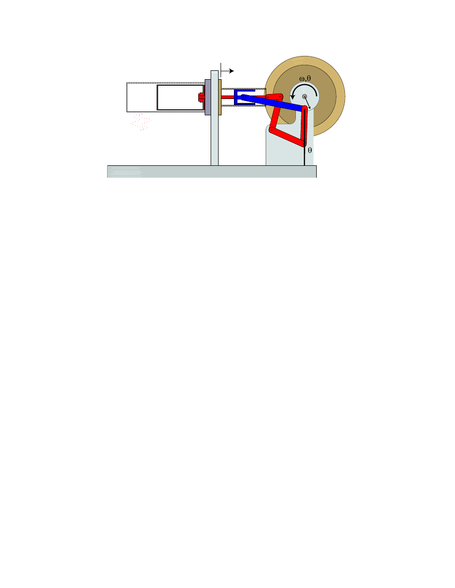
Figure 1: Schematic of Stirling Engine with key variables noted.

Introduction

In the undergraduate class 2.670 at M.I.T., the students explore basic manufacturing tech­
niques by building a stirling engine. The class is concluded by all of the students running
their engines at the same time. As the students discover, the stirling engine is very sensi­
tive to manufacturing tolerance, specifically the fit of the components determines both the
friction in the engine and air leakage out of the engine. The purpose of this project was
to develop a model of the stirling engine that accurately predicts the effects of leakage and
friction on engine performance.

1 Stirling Engines

Figure 1 shows a simple schematic of a stirling engine with key parameters noted. The
concept of a stirling engine is fairly simple. The engine consist of heat source, in our case
an alcohol flame, and a heat sink, ambient air, an enclosed cylinder, a ”heat” piston, a
”power” piston, and a flywheel connected to the two pistons by a set of linkages. The
concept is that the heat flowing through the air in the enclosed cylinder is modulate by the
position of the ”heat” piston. When the ”heat” piston is located directly over the flame the
heat flow into the engine is minimized while the heat flow out of the cylinder to the heat
sink is maximized. Similarly, when heat flow in is maximize, heat flow out is minimized.
While the ”heat” piston is moving, the ”power” piston is also moving thus converting the
thermal energy being captured by the air into mechanical motion. The flywheel then stores
this mechanical energy, thus allowing the mechanical power to flow both in and out of the
engine. The geometry of the linkages determines the relationship between the motion of the
”power” piston and the ”heat” piston.

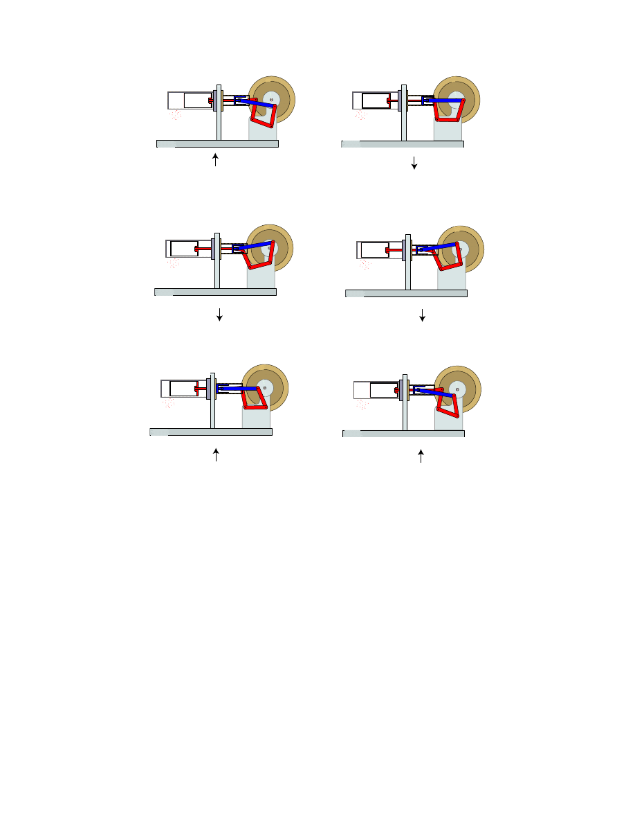
Figure 2 shows an animation of the stirling engine in operation. Frame A shows the engine

in the starting angular position. In the starting position, we see that the ”heat” cylinder

S

S

S

S

S

S

A

B

C

D

E

F

Figure 2: Animation of stirling engine in operation.

is positioned to maximize the heat in-flow while at the same time the ”power” piston is
positioned to maximize output power. In frame B, we see the engine has rotated such that
output power is minimized while the heat input area is reducing. In frame C, we see that
heat outflow is nearing maximum while mechanical power may actually be flowing back into
the engine. Frames D and E, show the transition back to heat in flow and mechanical power
outflow. Frame F shows the engine moving back into the maximum thermal power in and
mechanical power out position. I would like to thank Katherine Lilienkamp
for allowing me to use her matlab code to generate these animations.

From the 2.670 class notes by Prof. David Hart [1], the stirling engine built in the class

operates with a hot temperature, T

h

, of 600 K and a cold temperature, T

c

, of 300 K. The

typical engine will produce 1 W at 400 Rpm. The typical engine will operate at between
400-600 Rpm, with exceptional engines running at speeds up to 1200 Rpm.

C

1

TF

1

MTF

1

R

I

0

0

R

Se:Pa

R

Se:Th

R

Se:Ta

R*cos

x

Ap

V

Sa

Na

Te

Sh

Sc

Ah( )

Ac( )

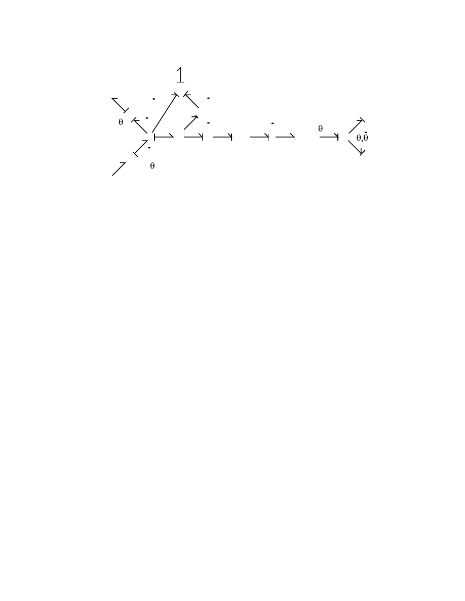
Figure 3: Bond graph model of stirling engine.

2 Stirling Engine Model

Figure 3 shows the bond graph model developed for the stirling engine. The heat source is
modelled a constant temperature effort source, T

h

, which transfers entropy to the air in the

cylinder, modelled as a multi-port capacitor, through a variable resistor. Similarly, the heat
sink is modelled as a constant temperature effort source, T

c

, which also transfers entropy to

the air in the cylinder through a different variable resistor. As mentioned earlier, the air in
the cylinder is modelled as a multi-port capacitor. Since leakage from the cylinder is impor­
tant, one port on the multi-port capacitor tracks the mass loss through a resitor to ambient
conditions, modelled as a constant pressure effort source. A second port on the capacitor
tracks the entropy flows too and from the heat sources and the entropy loss due to mass
flow. The final port on the capacitor is associated with the volume change. The pressure in
the cylinder acts upon the power piston which is modelled as a constant transformer. The
piston then acts upon the linkage to the flywheel, modelled as a modulated transformer.
Finally, the flywheel is modelled as an inertia, while all of the friction losses in the system
are modelled as a resistor with damping b. The major modelling assumption used in this

bond graph are:

• No power transfer through the ”heat” piston.
• Mass-less pistons.
• Uniform temperature for air in engine.
• Lumped friction element to govern engine speed.
• Uniform constant temperature sources.
• All leakage from engine through power cylinder.
• Motion of ”heat” piston is sinusoid 90 degrees ahead of power piston.

There are four state variable in this system.

θ

the angular position of the flywheel

θ˙

the angular velocity of the flywheel

S

e

the total entropy of the air in the cylinder

N

e

the number of mols of air contained in the cylinder

The model results in the following formulation equations:

x = R

e

(1 + sin θ)

A

h

= A

sc

(1 + cos θ)

A

c

= A

sc

(1 − cos θ) + P

ps

x

S˙

h

=

A

h

µ(T

h

− T

e

)

T

e

S˙

c

=

A

c

µ(T

e

− T

c

)

T

e

˙

N

e

= −A

l

�

2ρ

e

(P

e

− P

a

) or A

l

�

2ρ

a

(P

a

− P

e

)

˙

S

e

˙

S

a

=

N

a

N

e

S˙

e

= S˙

h

− S˙

c

+ S˙

a

V

e

= V

c

+ A

p

x

V

e

v¯

e

=

mN

e

�

−R

�

v¯

e

Cv

s¯

e

− s¯

o

T

e

= T

o

exp

v¯

o

C

v

�

v¯

e

�

−

(

−R

+1

)

s¯

e

− s¯

o

Cv

P

e

= P

o

exp

v¯

o

C

v

F

e

= (P

e

− P

a

)A

p

τ

e

= F

e

R

e

cos θ

τ

I

= τ

e

− bθ˙

¨

τ

e

− bθ˙

θ =

I

Where:

R

e

= 1.25 cm = Radius of linkage pivot on flywheel

A

sc

= 40 cm

2

= Heat transfer surface area of cylinder

P

pc

= 4.9 cm = Perimeter of power piston

A

h

= variable = Hot heat transfer area

A

c

= variable = Cold heat transfer area

T

e

= variable = temp of air in engine

µ

= 100000 W/m

2

= heat transfer constant of cylinder, this was calculated as

the thermal conductance of steel with the cylinder wall thickness

A

l

= nominally 0.06 mm

2

= area of leak

A

p

= 1.9 cm

2

= area of power piston

V

c

= 40 cm

3

= volume of air cylinder

m

= 29 kg/kmol = molar mass of air

R

= 287 J/kg = mass gas constant air

s¯

o

= 2800 J/K*kg = specific entropy of air at T=300 K

T

o

= 300 K = starting temp of air in cylinder

P

o

= P

a

= 1e5 Pa = ambient pressure

C

v

= 717 J/kg*K = constant volume specific heat

b

= 0.7e-3 N/rad/s = damping constant

I

= 4 kg ∗ cm

2

= inertia of flywheel

Values for thermal conductance from [2]. Values for thermal dynamic properties from

[3].

Initial Conditions

The model stirling engine was initialize at ambient thermal and pressure conditions. To
start the stirling engine in motion, a short duration (0.1 s) and small magnitude external
torque (0.1 N*m = 0.6 lbf*in) was applied to the flywheel. This is sufficient to accelerate the
flywheel to a nominal velocity of 500 Rpm. Further exploration showed that a nominal motor
would start with an initial velocity of 60 Rpm but the rise time to steady state operation was
on the order of 15 seconds. This long rise time resulted in impractically long computational
runs, thus for convenience the large initial velocity is used. Both large and small initial
velocities resulted in the same steady state velocity.

3 Results

For this project, I evaluated the two variables that the 2.670 students have the most control
over when building their motors. First is to evaluate the fit of the power piston into the
power cylinder (Note: in my model I assumed all of the leakage occurred at this interface
but leakage occurs at other spots). I ran the simulation with no leakage, a leakage area of
0.06 mm

2

(the equivalent to having to having a 2.54 µm gap between the piston and cylinder

wall), and a leakage area of 0.1 mm

2

(5 µm gap). While these gaps are smaller than I would

expect in actual motors, my model does not take into account the flow resistance caused by

0

0.5

1

1.5

2

2.5

3

3.5

4

4.5

5

0

100

200

300

400

500

600

700

800

900

Rotational Speed vs Time

Time (s)

S

p

e

e

d

(

R

p

m

)

No leakage

Leakage Area = 0.06 mm

Leakage Area = 0.1 mm

2

2

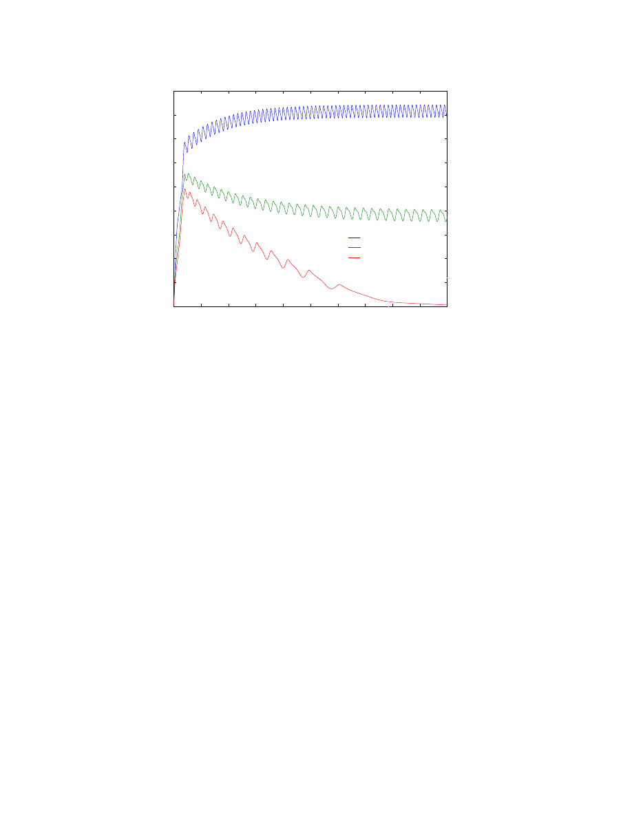
Figure 4: Rotational Speed vs Time for various leakage areas.

long interface between the piston and the cylinder (length of interface ≈ 1000x gap). My
modelling assumptions thus result in very small gaps allowing large flow.

The results for these three different leakage areas are shown in figures 4, 5, and 6. In

figure 4, we see rotational speed of the motor in Rpm vs time. As we expected, the steady
state velocity of the motor drops as leakage increases. In fact, a very small leakage results
in the motor not running. The no leak case has a terminal speed of 800 rpm with an output
power of 3.5 W. While the nominal motor, leakage area of 0.06 mm

2

, has a steady state

speed of 400 rpm with a corresponding power output of 1 W. Figure 5 shows the plot of
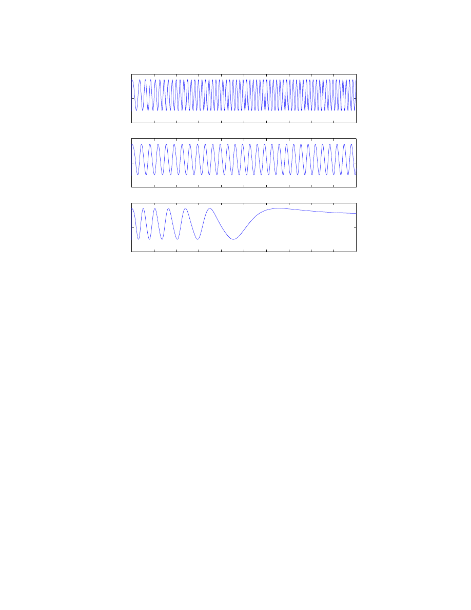
temperature vs time for all three leakage cases. All of the motors operate between 550 K
and 300 K. The size of this oscillation is most likely greater than that in an actual motor
because the actual motor has quite a bit of additional thermal storage that is not included in
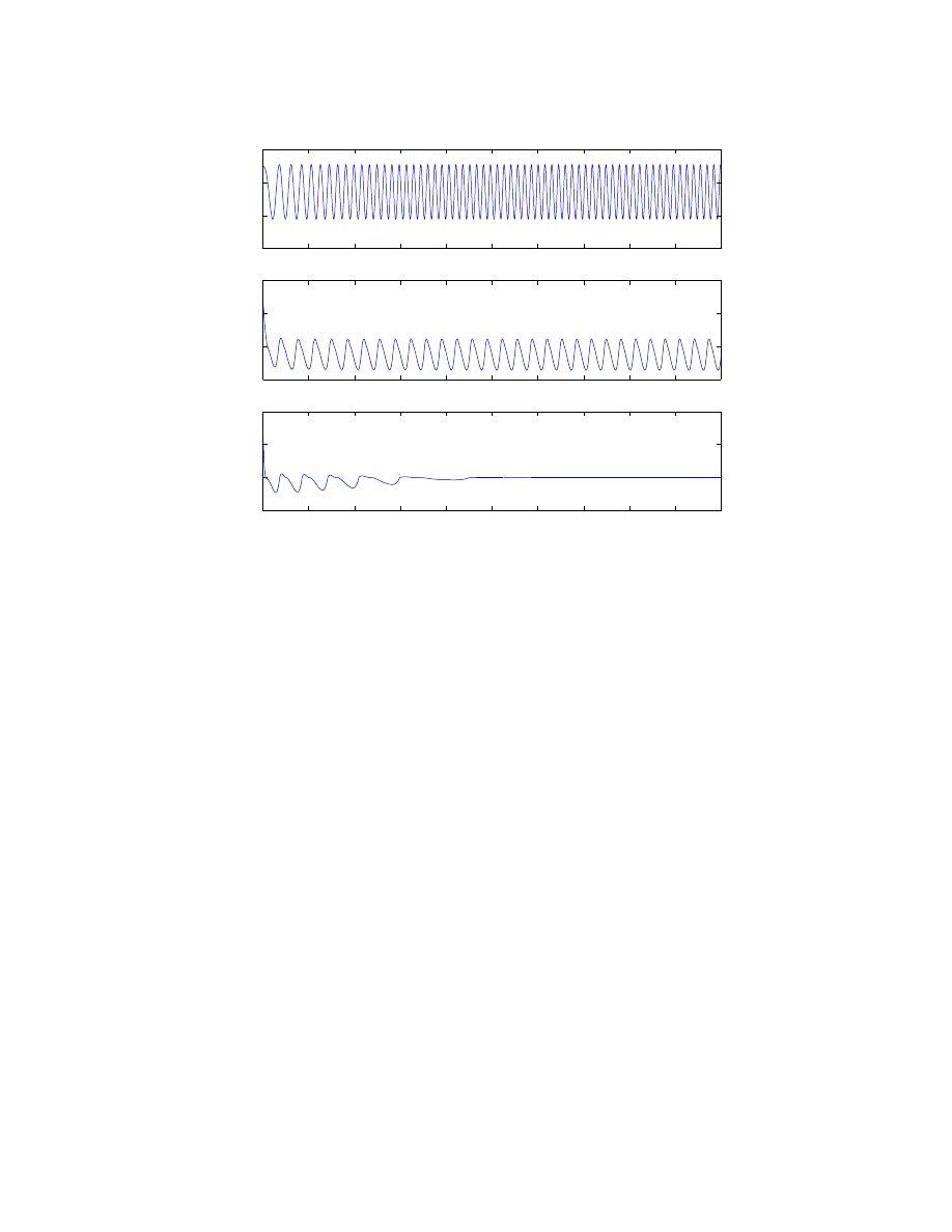
my model. Figure 6 shows the pressure vs time relationship for the three leakage cases. As
expected, the motor with no leakage operates at much higher pressures than the two motors
with leakage. Also as expected, the motor with leakage operate around ambient pressure.

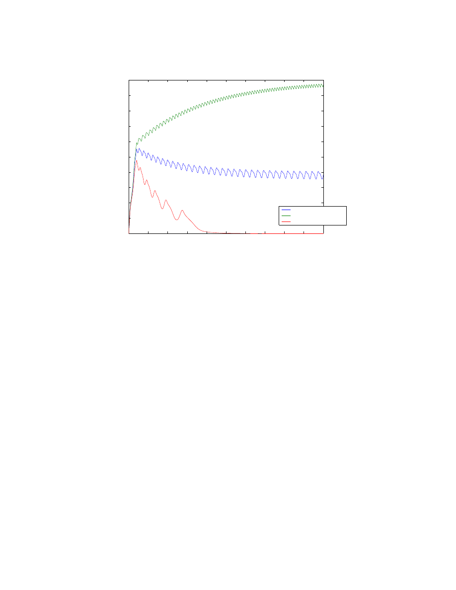
The second variable that I evaluated was to change the friction in the engine by changing

the viscous damping on the flywheel. Figure 7 shows the rotation speed vs time plots for
the nominal leakage motor for nominal friction, 50% friction, and 200% friction. As the plot
shows the terminal speed for the 50% friction motor is 950 rpm with a corresponding power
output of 2.4 W. While the 200% friction motor does not spin.

0

0.5

1

1.5

2

2.5

3

3.5

4

4.5

5

200

400

600

Temperature vs Time for various leakage areas

No Leakage

T

e

m

p

e

ra

tu

re

(

K

)

0

0.5

1

1.5

2

2.5

3

3.5

4

4.5

5

200

400

600

Leakage Area = 0.06 mm

2

T

e

m

p

e

ra

tu

re

(

K

)

0

0.5

1

1.5

2

2.5

3

3.5

4

4.5

5

200

400

600

Leakage Area = 0.1 mm

2

Time (s)

T

e

m

p

e

ra

tu

re

(

K

)

Figure 5: Temperature vs Time for various leakage areas.

Conclusions

In general, I am pleased with the results of this term project. The simulated system responds
appropriately to changes in the leakage and system friction. The model would likely by
improved with the incorporation of additional thermal storage elements and a better model
of leakage (thus allowing more realistic air gaps). Specifically, I would try to determine how
to add the thermal storage of the air in the ”heat” cylinder. Given the difficulties that I had
in setting up the simulated system with both the correct constitutive equations and system
parameters (I still do not know what was wrong with the .m file that failed with no heat
input), I am extremely pleased with these results.

References

[1] Hart, D. P. Stirling Engine Analysis 2.670 Course notes, Department of Mechanical

Engineering, Massachusetts Institute of Technology, Cambridge, MA, 1999 and 1997.

[2] White, Frank. Heat and Mass Transfer Addison-Wesley Publications, 1988.

[3] Van Wylen, G., Sonntag, R. Fundamentals of Classical Thermodynamics 3rd John

Wiley & Sons, Inc, New York, 1986.

0

0.5

1

1.5

2

2.5

3

3.5

4

4.5

5

0.5

1

1.5

2

x 10

5

Pressure vs Time for various leakage areas

No Leakage

Pressure (Pa)

0

0.5

1

1.5

2

2.5

3

3.5

4

4.5

5

0.5

1

1.5

2

x 10

5

Leakage area = 0.06 mm

2

Pressure (Pa)

0

0.5

1

1.5

2

2.5

3

3.5

4

4.5

5

0.5

1

1.5

2

x 10

5

Leakage area = 0.1 mm

2

Time (s)

Pressure (Pa)

Figure 6: Pressure vs Time for various leakage areas.

A Matlab file for model parameters

%
%Stirling Engine Simulation
%Th=Hot temp, Tc=ambient temp, Tg=gas temp, Ae=end area, As=cylinder area T
%Asc=area power cylinder, Al=leakage area, rf=radius of pivot, mu=heat transfer
clear all; close all; global Th Tc Ae As Al rf mu Apc Veo R Cv Pa
so Pp If b M Ts qa qo vo
rf=0.5*2.5/100; %radius of power linkage
Ae=(1.25*2.5)^2*pi/(4*100^2); %area of heat cylinder end plate
As=(1.25*2.5*pi*1.5*2.5/100^2); %area of oscillating portion
Apc=(0.625*2.5)^2*pi/(4*100^2); %power cylinder area
Pp=(0.625*2.5*pi/100); %power cylinder perimeter
mu=100000; %heat transfer coefficient W/K*m^2
Veo=pi*((3.69*2.5*(1.225*2.5/2)^2-2.5*2*(1.060*2.5/2)^2))/100^3;
%base volume for engine
R=287; Cv=716; Pa=1e5; so=2800;
Al=pi*((2.5*.625)^2-(2.5*.6249)^2)/(4*100^2); %leak area
If=4/(100^2);%kg*m^2 inertia of flywheel
Th=600; %hot temp

0

0.5

1

1.5

2

2.5

3

3.5

4

4.5

5

0

100

200

300

400

500

600

700

800

900

1000

Rotation Speed vs Time for three different frictional losses

Leakage Area = 0.06 mm

2

Time(s)

R

o

ta

tio

n

a

l S

p

e

e

d

(

R

p

m

)

Nominal Friction
Friction 1/2 nominal
Friction twice nominal

Figure 7: Rotational Speed vs Time for various motor frictions.

Tc=300; %cold temp
Ts=300;
b=560e-6; %rotational damping N*m/rad/s
M=29; ni=Pa*(Veo+Apc*12.5e-3)/(Ts*R*M); Veo=(Veo+Apc*12.5e-3);
vo=Veo/(ni*M); si=ni*M*so; qa=Pa/(R*M*Tc); yi=[0 si ni 0];

options=odeset(’MaxStep’,0.001);

[t,y]=ode15s(@stirling,[0 5],yi,options);

B Matlab function for Stirling Engine simulation

function dy=stirling(t,y);

global Th Tc Ae As Asc Al rf mu Apc Veo R Cv Pa so Pp If b M Ts qa
qo vo
%y(1)=angle y(2)=engine entropy y(3)=moles gas y(4)=flywheel speed
dy=zeros(4,1);

x=12.5e-3*(1+sin(y(1)));
ve=Veo+x*Apc;

Ah=As*(1+cos(y(1)));
Ac=As*(1-cos(y(1)))+Pp*x+Ae;
ve=ve/(y(3)*M);
se=y(2)/(y(3)*M);
Te=Ts*(ve/vo)^(-R/Cv)*exp((se-so)/Cv);
Pe=Pa*(ve/vo)^(-(R/Cv+1))*exp((se-so)/Cv); dsh=mu*Ah*(Th-Te)/Te;
dsc=mu*Ac*(Te-Tc)/Te; if Pe>Pa

dn=-Al*sqrt(2*(Pe-Pa)/ve);

else

dn=Al*sqrt(2*(Pa-Pe)*qa);

end if (t>0)&(t<0.1)

tau=0.1;

else

tau=0;

end

dsa=(y(2)/(M*y(3)))*dn;
dy(2)=dsh-dsc+dsa;
dy(3)=dn;
dy(4)=((Pe-Pa)*Apc*rf*cos(y(1))-b*y(4)+tau)/If;

dy(1)=y(4);