Portfolio Optimization Under Value At Risk Constraint

Portfolio optimization under

value-at-risk constraint

Traian A Pirvu

Department of Mathematics

The University of British Columbia

Vancouver, BC, V6T1Z2

tpirvu@math.ubc.ca

October 21, 2005

Abstract

In this paper, we analyze the effects arising from imposing a Value-at-Risk con-
straint in an agent’s consumption and portfolio selection problem. The market
consists of m risky assets (stocks) plus a risk free asset. The stocks are modelled
as exponential Brownian motions with random drift and volatility. The risk of the
trading portfolio and consumption is reevaluated dynamically and hence the agent
must satisfy the Value-at-Risk constraint continuously. We derive the optimal con-
sumption and portfolio allocation policy in closed form for the case of logarithmic
utility. The problem for general power utility is reduced to a deterministic control
one, which is analyzed and solved numerically. The VaR constraint remains active
once it becomes active and reduces the consumption and investment in the risky
assets. The optimal policies are projections of the optimal unconstrained ones onto
the constraint set.

JEL classification: G10
Mathematics Subject Classification (2000): 91B30, 60H30, 60G44

Introduction

Managers limit the riskiness of their traders by imposing limits on the risk of their portfo-
lios. Lately, the Value-at-Risk (VaR) risk measure has became a tool used to accomplish this
purpose. The increased popularity of this risk measure is due to the fact that VaR is easily un-
derstood. It is the maximum loss of a portfolio over a given horizon, at a given confidence level.
The Basle Committee on Banking Supervision requires U.S. banks to use VaR in determining
the minimum capital required for their trading portfolios.

Basak and Shapiro (2001) analyze the optimal dynamic portfolio and wealth-consumption

policies of utility maximizing investors who must manage risk exposure using VaR. They find
that VaR risk managers pick a larger exposure to risky assets than non-risk managers, and

Work supported by NSERC under research grant 88051 and NCE grant 30354 (MITACS).

consequently incur larger losses when losses occur. In order to fix this deficiency they choose
another risk measure based on the risk-neutral expectation of a loss. They called this risk
measure Limited Expected Loss (LEL). One drawback of their model is that the portfolios VaR
is never reevaluated after the initial date, making the problem a static one. In a similar setup,
Berkelaar, Cumperayot and Kouwenberg (2002) show that VaR reduces market volatility, but
in some cases raises the probability of extreme losses. Emmer, Kl¨

uppelberg and Korn (2001)

consider a dynamic model with Capital-at-Risk (a version of VaR) limits. However, they
assume that portfolio proportions are held fixed during the whole investment horizon and thus
the problem becomes a static one as well.

Cuoco, He and Issaenko (2001) develop a more realistic dynamically-consistent model of

the optimal behavior of a trader subject to risk constraints. They assume that the risk of
the trading portfolio is reevaluated dynamically by using the conditioning information, and
hence the trader must satisfy the risk limits continuously. Another assumption they make
is that when assessing the risk of a portfolio, the distribution of the portfolio composition is
kept unchanged over a given horizon (more exactly the proportions of different assets are kept
unchanged). Besides VaR risk measure, they consider a coherent risk measure Tail value at
Risk (TVaR), and establish that it is possible to identify a dynamic VaR risk limit equivalent
to a dynamic TVaR limit. Another of their findings is that the risk exposure of a trader subject
to VaR and TVaR limits is always lower than that of an unconstrained trader.

In my Ph.D. thesis Pirvu (2005) we start with the model of Cuocco, He and Issaenko

(2001). We find the optimal growth portfolio subject to these risk measures. Our main finding
is that the optimal policy is a projection of the optimal portfolio of an unconstrained log agent
(the Merton proportion) onto the constraint set with respect to the inner product induced by
the variance-covariance volatilities matrix of the risky assets. We manage to get closed-form
solutions even when the constraint set depends on the current wealth level. We extend the
model from the constant coefficient market to one with random coefficients.

In his Ph.D. thesis Rivera (2004) considers a similar model, but he chooses to keep the

actual number of shares unchanged, rather than the proportion. He solves the investment
problem in a general semimartingale market model. Cuoco and Liu (2001) study the dynamic
investment and reporting problem of a financial institution subject to capital requirements
based on self-reported VaR estimates. For a market with constant price coefficients, they show
that optimal portfolios display a local three-fund property. Leippold, Trojani and Vanini (2002)
analyse VaR-based regulation rules and their possible distortion effects on financial markets.
They show that in partial equilibrium the effectivnes of VaR regulation is closely linked to the
leverage effect, the tendency of volatility to increase when the prices decline.

Yiu K.F.C. (2004) looks at the optimal portfolio problem, when an economic agent is

maximizing utility of her intemporal consumption over a period of time under a dynamic VaR
constraint. A numerical method is proposed to solve the corresponding HJB-equation. He
finds that investment in risky assets are optimally reduced by the VaR constraint. Atkinson
and Papakokkinou (2005) derive the solution to the optimal portfolio and consumption subject
to CaR and VaR constraints by using stochastic dynamic programming.

This paper extends Pirvu (2005) by allowing for intertemporal consumption. We address

an issue raised in Yiu K.F.C. (2004) and Atkinson and Papakokkinou (2005) by considering
a market with random coefficients. Section 2 describes the model, including the definition
of Value-at-Risk constraint. Section 3 formulates the objective problem and it shows the

limitations of the stochastic dynamic programming approach. Section 4 treats the special case
of logarithmic utility. The problem of maximizing expected logarithmic utility of intertemporal
consumption is solved in closed form solutions. This is done by reducing it to an optimization
problem which is solved pathwise. One finding is that at the final time the agent invests the
least proportion of her wealth in stocks. The optimal policy is a projection of the optimal
portfolio and consumption of an unconstrained agent onto the constraint set. After some
time VaR constraint starts being active and it remains active. Section 5 treats the case of
power utility. The portfolio and consumption problem is reduced to a deterministic control
one. We establish existence of an optimal solution for it. We characterized the solutions by
Pontryagin maximum principle (first order necessary conditions). Then it is shown that the
necessary conditions are also sufficient. Section 8 contains an appropriate discretization of the
deterministic control problem. It leads to a nonlinear program which can be solved by standard
methods. It turns out that the necessary conditions of the discretized problem converges to the
necessary conditions of the continuous problem. We conclude the paper with some numerical
experiments done with AMPL, a nonlinear programming solver.

The Model

2.1

Stocks

We consider a market whose risk-free interest rate r is positive and which has multiple risky
assets. There are m stocks driven by n independent Brownian motions. Here we assume
m ≤ n, i.e., there are at least as many sources of uncertainty as assets:

(t) = S

(t)



α

(t) dt +

j=1

(t) dW

(t)



 , 0 ≤ t ≤ ∞, i = 1, . . . , m.

• the drift process α(·) is assumed positive and continuous.

• the matrix-valued volatility process σ(·) is assumed continuous and with linearly inde-

pendent rows.

We define the excess rates of return µ

(t) = α

(t) − r, which are assumed positive. We denote

by µ(t) = (µ

(t)) the column vector of excess rates of return and by W (t) = (W

(t)) the column

vector of independent Brownian motions on a filtered probability space (Ω, {F

}

0≤t≤T

, F, P).

2.2

Wealth

Let ζ

(t) denote the proportion of an agent’s wealth in stock i at time t, and let ζ(t) = (ζ

(t))

denote the column vector of proportions. The intermediate consumption process is denoted
C(t) and is assumed positive and adapted. The agent’s wealth is then given by

dX(t) = X(t)

£¡

r − c(t) + ζ

(t)µ(t)

dt + ζ

(t)σ(t) dW (t)

where c(t) =

C(t)

X(t)

is the expenditure rate. Define

Q(t, ζ, c) , r − c + ζ

µ(t) −

1
2

|ζ

σ(t)|

(2.1)

and for each number p < 1 define

(t, ζ, c) , r − c + ζ

µ(t) +

p − 1

|ζ

σ(t)|

(2.2)

Then

X(t) = X(0) exp

½Z

u, ζ(u), c(u)

du +

(u)σ(u) dW (u)

(2.3)

2.3

Value-At-Risk Limits

For a given path ω lets denote ω

(t)

= (ω

)

s≤t

the projection up to time t of its trajectory.

Starting at time t, for a fixed ω

(t)

, hold the proportions ζ and c constants over a time interval

of length τ > 0 and imagine that the processes µ(·) and σ(·) will remain fixed over the time
interval [t, t + τ ], holding the values they have at t. Then

X(t + τ ) = X(t) exp

Q(t, ζ, c)τ + ζ

σ(t)

W (t + τ ) − W (t)

¢ª

X(t) − X(t + τ ) = X(t)

1 − exp

Q(t, ζ, c)τ + ζ

σ(t)

W (t + τ ) − W (t)

¢ª¤

For a fixed ω

(t)

, the random variable ζ

σ(t)

W (t + τ ) − W (t)

is normal with mean zero and

standard deviation |ζ

σ(t)|

√

τ , we can write it as Y |ζ

σ(t)|

√

τ , where Y is a standard normal.

We lose money when this is small, in which case X(t) − X(t + τ ) is large. Let α ∈ (0,

] be

given. The α-percentile of X(t) − X(t + τ ) is

X(t)

1 − exp

Q(t, ζ, c)τ + N

−1

(α)|ζ

σ(t)|

√

ª¤

where N (·) denotes the standard cumulative normal distribution function. This will lead to
the following definitions:

VaR

α,ζ,c

(t, x) ,

1 − exp

Q(t, ζ, c)τ + N

−1

(α)|ζ

σ(t)|

√

ª¤

We fix a constant a

∈ (0, 1). The Value-at-Risk constraint is that at every time t ≥ 0 the

agent must choose a portfolio proportion ζ(t) and an expenditure rate c(t) in the set F

(t)

defined by

(t) ,

ζ ∈ R

, c ≥ 0 : VaR

α,ζ,c

(t, x) ≤ a

(2.4)

Note that this set depend on the path ω

(t)

. We notice that for fixed ω

(t)

and fixed time t, the

set F

(t)(ω

(t)

) is compact and convex, being the level set of the following convex, unbounded

function:

(t, ζ, c) , −Q(t, ζ, c)τ − N

−1

(α)|ζ

σ(t)|

√

τ ,

(2.5)

(t) =

ζ ∈ R

, c ≥ 0 : f

(t, ζ, c) ≤ log

1 − a

Because α ∈ (0,

], N

−1

(α) ≤ 0 and hence the function f

is convex.

Objective

Given a finite time horizon T and a positive initial wealth X(0), an agent seeks to choose a
portfolio proportion process ζ(t), and an expenditure rate process c(t) t ≥ 0, so that X(t) > 0
and (ζ(t), c(t)) ∈ F

(t) for all 0 ≤ t ≤ T almost surely so that the expected value of the

random variable

−δt

(C(t))dt + e

−δT

(X(T )),

(3.6)

is maximized over all portfolio proportions and expenditure rates processes satisfying the same
constraints. Here U

, and U

are utility functions. In other words the agent facing VaR

constraints is deriving utility from the intermediate consumption and from terminal wealth
process. Let us notice that the constraints are enforced at the final time T as well. We consider
also the case of deriving utility from the intermediate consumption only. This corresponds to
maximizing

−δt

(C(t))dt,

(3.7)

over the constraint sets. Maximizing expected utility of the final wealth under VaR and other
types of risk constraints was considered in my Ph.D thesis [16]. Let us assume for the moment
that the market coefficients are constant. In this case the constraint set F

(t) does not depend

on time and we denote it F

. Then one can use the dynamic programming techniques to

characterize the optimal portfolio and consumption policy. The problem is to find a solution
to the HJB-equation. Define the optimal value function as

V (x, t) = max

(ζ,c)∈F

·Z

−δt

(C(t))dt + e

−δT

(X(T ))

where E

is the conditional operator given the information known up to time t and X(t) = x.

The HJB equation is

max

(ζ,c)∈F

J(t, x, ζ, c) = 0,

where

J(t, x, c, ζ) , e

−δt

(cx) +

∂V

∂t

+ x(r − c + ζ

µ)

∂V

∂x

|ζ

σ|

∂

∂x

with boundary the condition V (x, T ) = e

−δT

(x). The value function V inherits the concavity

from the utility functions U

and U

. It is obvious that the function J is jointly concave on ζ, c

so it is maximized over the set F

at a unique point (ζ, c). Moreover this point should lie on

the boundary of F

and one can derive first order conditions by means of Lagrange multipliers.

Together with the HJB equation yield a highly nonlinear system which is hard to solve even
numerically. If the market coefficients are random one cannot derive HJB equations unless
the coefficients are functions of some state variables. In what follows we tackle the portfolio
optimization problem by reducing it to a deterministic control problem. Our method, however
works only for the case U

(x) = U

(x) =

, where p < 1 is the coefficient of relative risk

aversion (CRRA). We are able to solve the portfolio problem in closed form for logarithmic
utility.

Logarithmic utility

For the sake of simplicity let us consider the case in which the agent is deriving utility from
intermediate consumption only. Itˆo’s lemma applied to the wealth process X(t) gives:

log X(t) = log X(0) +

Q(s, ζ(s), c(s))ds +

(s)σ(s) dW (s).

(4.8)

Thus

−δt

log C(t)dt =

−δt

log (c(t)X(t))dt =

1 − e

−δT

log X(0) +

−δt

log c(t)dt

−δt

Q(s, ζ(s), c(s))dsdt +

−δt

(s)σ(s) dW (s)dt.

By Fubini’s Theorem

−δt

Q(s, ζ(s), c(s))dsdt =

µZ

−δt

Q(s, ζ(s), c(s))dt

−δt

− e

−δT

Q(t, ζ(t), c(t))dt,

hence
Z

−δt

log C(t)dt =

1 − e

−δT

log X(0)+

−δt

log c(t) +

1
δ

(1 − e

−δ(T −t)

)Q(t, ζ(t), c(t))

−δt

(s)σ(s) dW (s)dt.

(4.9)

Let ζ

(t) , (σ(t)σ

(t))

−1

µ(t) be the optimal portfolio proportion (for log utility) in the

absence of risk constraints. Let us assume that

|ζ

(u)σ(u)|

du < ∞.

(4.10)

Lemma 4.1 For every (ζ(t), c(t)) ∈ F

(t) the process

(s)σ(s) dW (s), where t ∈ [0, T ] is

a martingale.

Proof: In order to prove the martingale property of

(s)σ(s) dW (s) it suffices to show

|ζ

(u)σ(u)|

du < ∞.

(4.11)

Let us notice that

|ζ

(t)µ(t)| = |ζ

(t)σ(t)σ

(t)ζ

(t)| ≤ |ζ

(t)σ(t)| · |ζ

(t)σ(t)|.

(4.12)

For (ζ(t), c(t)) ∈ F

(t), we have

r − c(t) + ζ

(t)µ(t) −

1
2

|ζ

(t)σ(t)|

τ + N

−1

(α)|ζ

(t)σ(t)|

√

τ ≥ log(1 − a

This combined with (4.12) gives

|ζ

(t)σ(t)| ≤ k

+ k

∨ |ζ

(t)σ(t)|,

(4.13)

for some positive constants k

and k

. In the light of the assumption (4.10) the inequality

(4.11) follows.

The above Lemma implies

−δt

(s)σ(s) dW (s)dt = 0

after interchanging the order of integration. The identity (4.9) becomes

−δt

log X(t)dt =

1 − e

−δT

log X(0)+E

−δt

log c(t) +

1
δ

(1 − e

−δ(T −t)

)Q(t, ζ(t), c(t))

dt.

Therefore to maximize

−δt

log C(t)dt,

over the constraint set it suffices to maximize

log c(t) +

1
δ

(1 − e

−δ(T −t)

)Q(t, ζ(t), c(t))

pathwise over the constraint set.

Let us fix a path ω and a time t. The concave objective function

g(t, ζ, c) , log c +

1
δ

(1 − e

−δ(T −t)

)Q(t, ζ, c)

(4.14)

is maximized over R

m+1

by (ζ

(t), c

(t)), where c

(t) ,

1−e

−δ(T −t)

. If this point is in the

constraint set, then is the optimal solution. Otherwise the concave objective function is maxi-
mized over the compact, convex set at a unique point (ζ

(t), c

(t)); moreover, this point must

be on the boundary of F

(t). Hence it solves the optimization problem

(P 1)

maximize g(t, ζ, c)

subject to f

(t, ζ, c) , −Q(t, ζ, c)τ − N

−1

(α)|ζ

σ(t)|

√

τ = log

1−a

Let us assume that the optimal ζ

(t) is not the zero vector. According to the Lagrange

multiplier theorem, either ∇f

(t, ζ

(t), c

(t)) = 0 or else there is a positive λ(t) such that

∇g(t, ζ

(t), c

(t)) = λ(t)∇f

(t, ζ

(t), c

(t)).

(4.15)

Since

∇f

(t, ζ, c) =

(−µ + σ(t)σ(t)

ζ)τ −

−1

(α)

√

|ζ

σ(t)|

σ(t)σ(t)

ζ, τ

6= 0,

it follows

(t) = c

(t)(1 + λ(t)τ )

1 + λ(t)τ −

−1

(α)

√

|ζ

(t)σ(t)|

−1

(t),

(t) =

(t)

+ λ(t)τ

−1

This shows that the optimal solution (ζ

(t), c

(t)) also solves

(P 2)

maximize l(λ

, λ

)

subject to f

(t, λ

(t), λ

(t)) = log

1−a

where

l(λ

, λ

) , g(t, λ

(t), λ

(t)),

(4.16)

and the maximization is with respect to the positive λ

and λ

. This concave function is

maximized over R

by (1, 1). We know this point is not in the constraint set, hence the optimal

(λ

(t), λ

(t)) must satisfy

1 − λ

= −

β(t)c

(t)

|ζ

(t)σ(t)|

τ (1 − λ

)|ζ

(t)σ(t)|

√

τ N

−1

(α)|ζ

(t)σ(t)|

(4.17)

− 1 = β(t)τ c

(t),

(4.18)

for a positive Lagrange multiplier β(t). By dividing the two identities we can eliminate β(t)
and get λ

= u(t, λ

), where

u(t, x) , 1 +

√

τ |ζ

(t)σ(t)|

−1

(α)

(1 − x).

(4.19)

Therefore λ

= λ

(t) is a root of the equation

(t, xζ

(t), u(t, x)c

(t)) = log

1 − a

(4.20)

in the variable x. The function h(t, x) , f

(t, xζ

(t), u(t, x)c

(t)) − log

1−a

is convex, un-

bounded in x and h

t, 1 +

−1

(α)

|ζ

(t)σ(t)|

√

≤ 0. This shows that the equation (4.20) has a unique

root λ

(t) > 1 +

−1

(α)

|ζ

(t)σ(t)|

√

. If h(t, x) ≤ 0 this root is nonnegative. Otherwise λ

(t) < 0 and

this is a contradiction. In this case

0, r +

log

1−a

is the optimal solution and

r +

log

1 − a

≤ c

(t) ,

1 − e

−δ(T −t)

Moreover h(t, 1) < 0 since we assumed (c

(t), ζ

(t)) is not in the constraint set and this

implies λ

(t) < 1. We argue that if λ

(t) > 0 then ζ

(t) = λ

(t)ζ

(t), c

(t) = u(t, λ

(t))c

(t)

is the optimal solution. Since it satisfies the first order conditions and the function l defined
by (4.16) is strictly concave, (ζ

(t), c

(t)) solves the following perturbed problem.

(P 2 ²)

maximize l(λ

, λ

)

subject to f

(t, λ

(t), λ

(t)) ≤ log

1−a

, λ

≥ ²,

for a small positive ². Let us assume that

0, r +

log

1−a

is the optimal solution for P 1.

Consider a point ζ

(t) = δ

(t), c

(t) = δ

(t) on the line segment joining

0, r +

log

1−a

and (ζ

(t), c

(t)), with f

(t, δ

(t), δ

(t)) ≤ log

1−a

and δ

≥ ². Then by the strict con-

cavity of the objective function g, (see (4.14)) one has l(δ

, δ

) > l(λ

(t), u(t, λ

(t))c

(t)),

which contradicts optimality of (ζ

(t), c

(t)) for the problem P 2 ². At this point we are ready

to state the following theorem.

Theorem 4.2 The problem of maximizing

−δt

log C(t)dt,

over processes (ζ(t), c(t)) ∈ F

(t), 0 ≤ t ≤ T, has the optimal solution

(t) = (1 ∧ (λ

(t) ∨ 0))ζ

(t),

(4.21)

(t) = u(t, (1 ∧ λ

(t)))c

(t)1

{λ

(t)>0}

r +

log

1 − a

{λ

(t)≤0}

(4.22)

where λ

(t) is the root of the equation (4.20), ζ

(t) , (σ(t)σ

(t))

−1

µ(t), c

(t) ,

1−e

−δ(T −t)

and the function u(·, ·) was defined in (4.19).

Proof: See the above analysis.

Remark 4.3 Since at the final time c

(T ) = ∞ and c

(T ) is bounded we must have λ

(T ) =

0 or otherwise λ

(T ) = 1+

−1

(α)

|ζ

(t)σ(t)|

√

. This shows that for a market with coefficients constants

in time ζ

(T ) ≤ ζ

(t), for any t ≤ T, (where the inequality is meant componentwise) and it

says that at the final time the agent invests the least proportion of her wealth in stocks. Note that
λ

(t) is an decreasing function in t since c

(t) is increasing. This says that once the constraint

starts being active it remains active. By (4.18) and (4.21) it follows that ζ

(t) ≤ ζ

(t), and

(t) ≤ c

(t), for any 0 ≤ t ≤ T. Therefore the solution for the constrained problem is a

projection of the solution for the unconstrained problem onto the constraint set. We can perform
some crossectional analysis. Let T

and T

two final times, T

> T

. Because c

(t, T

) <

(t, T

), from the equations (4.19) and (4.20) we conclude that λ

(t, T

) > λ

(t, T

), hence

(t, T

) > ζ

(t, T

), and c

(t, T

) > c

(t, T

). Therefore long-term agents can afford to invest

more in the stock market and consume more than short term agents (in terms of proportions).

Non-logarithmic utility

Let us recall that we want to maximize:

−δt

(t)

dt + Ee

−δT

(T )

(5.23)

and

−δt

(t)

dt,

(5.24)

over processes (ζ(t), c(t)) ∈ F

(t), 0 ≤ t ≤ T. Direct computations show:

(t) = X

(0) exp

µZ

pQ(s, ζ(s), c(s))ds +

pζ

(s)σ(s) dW (s)

= X

(0)M (t)Z(t),

where

M (t) , exp

µZ

(s, ζ(s), c(s)) ds

(5.25)

Z(t) , exp

−

1
2

|ζ

(s)σ(s)|

ds +

pζ

(s)σ(s) dW (s)

(5.26)

and Q, Q

were defined by (2.1) and (2.2). We assume that

·µ

exp

|ζ

(u)σ(u)|

¶¸

< ∞,

(5.27)

and market coefficients are totally unhedgeble, i.e. the drift process α(·) and the matrix-valued
volatility process σ(·) are assumed to be adapted to the filtration ˘

F(t) , σ( ˘

W (s), 0 ≤ s ≤ t),

generated by the m-dimensional Brownian motion ˘

W (·) = (W

n+1

(·), . . . , W

n+m

(·)), which is

assumed independent of the n-dimensional Brownian motion ˆ

W (·) = (W

(·), . . . , W

(·)). The

risk due to market coefficients cannot be hedged and the economic intuition is that the agent
should ignore it.

Lemma 5.1 For every ζ(t) ∈ F

(t) the process Z(t), where t ∈ [0, T ] is a martingale.

Proof: The assumption (5.27) combined with (4.13) and The Novikov Condition (see Karatzas and Shreve [12],
page 199, Corollary 5.13), makes the processes Z(t) a martingale.

One has

−δt

(t)

dt =

−δt

(t)

(t) dt

−δt

(t)

M (t)(Z(t) − Z(T )) dt + Z(T )

−δt

(t)

M (t) dt

Let us prove

−δt

(t)

M (t)(Z(t) − Z(T ))dt = 0.

By conditioning and Lemma 4.1 we get

E[c

(t)M (t)(Z(t) − Z(T ))] = E[E[c

(t)M (t)(Z(t) − Z(T ))|F

]]

= E[c

(t)M (t)[E(Z(t) − Z(T ))|F

]]

= 0,

and Fubini’s Theorem proves the claim. Hence

−δt

(t)

dt = E Z(T )

−δt

(t)

M (t)dt.

(5.28)

This suggests to maximize

−δt

(t)

M (t)dt,

(5.29)

and

−δt

(t)

M (t)dt + e

−δT

M (T )

(5.30)

pathwise over the constraint set for the case of an agent with CRRA p < 1, who derives utility
from intermediate consumption ( 5.23) and also from final wealth ( 5.24). Therefore we have
to analyze deterministic control problems.

5.1

Deterministic Control

In the language of deterministic control we can write (5.29) as a cost functional I[x, u] given
in the form

I[x, u] =

(t, x(t), u(t)) dt,

where u = (ζ, c) is the control and the function

(t, x, u) , e

−δt

(5.31)

is defined on the set

A = {(t, x, u)|(t, x) ∈ [0, T ] × (0, K], u ∈ F

(t)} ⊂ R

m+3

(5.32)

The state variable x is defined by the differential equation

= f (t, x(t), u(t)), 0 ≤ t ≤ T,

(5.33)

with the boundary condition x(0) = 1, where

f (t, x, u) , x(pr − pc + pζ

µ(t) +

p(p − 1)

|ζ

(t)σ(t)|

In fact

x(t) = e

(t,c(u),ζ(u)) du

(5.34)

with

(t, c, ζ) , pr − pc + pζ

µ(t) +

p(p − 1)

|ζ

σ(t)|

The constraints are (t, x(t)) ∈ [0, T ] × (0, K] and u(t) ∈ F

(t). Due to the compactness of

the set F

(t), 0 ≤ t ≤ T it follows that K < ∞. A pair (x, u) satisfying the above conditions

is called admissible. The problem of finding the maxima of I[x, u] within all admissible pairs

(x, u) is called the Lagrange problem of control. Alternatively for (5.30) we can consider the
cost functional I[x, u] given in the form

I[x, u] = g(x(T )) +

(t, x(t), u(t)) dt,

g(x) , e

−δT

(5.35)

together with the same differential equation and constraints as above. The problem of finding
the maxima of this functional is called the Bolza problem of control. We investigate the
existence of maximizers for these problems. The next step is to find out necessary conditions.
Then we question whether or not this conditions are also sufficient.

5.1.1

Existence

The classical existence theory for deterministic control problems involves the set

Q(t, x) , {(z

, z)|z

≥ −f

(t, x, u), z = f (t, x, u), u ∈ F

(t)}

(5.36)

The following theorem is known as the Fillipov existence theorem for Bolza and Lagrange
problems (see Theorem 9.3i in Cesari [5])

Theorem 5.2 Let the set A defined by (5.32) be compact, g lowersemicontinuous and f

(t, x, u)

and f (t, x, u) continuous on A. Let us assume that for almost all (t, x) ∈ [0, T ] × (0, K] the sets

Q(t, x) are convex. Then the functional I[x, u] given by (5.35) has an absolute maximum.

However in our case it is rather cumbersome to verify the convexity of ˜

Q(t, x) hence we

proceed with a direct proof of existence. Let us recall that for u(t) = (ζ(t), c(t)) ∈ F

(t),

|ζ

(t)σ(t)| ≤ k

+ k

∨ |ζ

(t)σ(t)|,

(5.37)

hence |ζ

(t)σ(t)| is uniformly bounded on [0, T ] due to the continuity of market coefficients.

Moreover one can conclude that |ζ(t)| ≤ M and c(t) ≤ M for some constant M. From (5.33)
by Gronwall’s Lemma x(t) ≤ N and ˙x(t) ≤ N on [0, T ] for some constant N.

Theorem 5.3 There exist a solution for the above control problems.

Proof: Let (x

(·), u

(·)) be a maximizing sequence, i.e. I[x

, u

] −→ sup I[x, u]. It is easily

seen that the sequence x

(·) is uniformly bounded and equicontinuous, thus Arzela-Ascoli

theorem gives uniform convergence to some function ˜

x(·). According to Kolmos Lemma (see

Lemma A1.1 in [8]) we can find some sequences of convex combinations ζ

∗

∈ conv(ζ

, ζ

n+1

, . . . )

and c

∗

∈ conv(c

, c

n+1

, . . . ) which converges a.e. to some measurable function ζ

∗

(·) and c

∗

(·),

such that u

∗

(t) , (ζ

∗

(t), c

∗

(t)) ∈ F

(t) , 0 ≤ t ≤ T, due to the convexity and compactness

of the sets F

(t). Let us denote x

∗

(·) the sequence of state variables corresponding to these

controls, i.e.,

∗

(t) = e

(t,c

∗

(s),ζ

∗

(s)) ds

, 0 ≤ t ≤ T,

(see (5.34)). Assume p > 0, the other case is similar. Due to the concavity of the function
f

, ln x

∗

(t) ≥ conv(ln x

(t), ln x

n+1

(t), . . . ), where the convex combination is the one defining

∗

, c

∗

. If y

∗

, exp(conv(ln x

(t), ln x

n+1

(t), . . . )), then x

∗

(t) ≥ y

∗

(t), and y

∗

(t) −→ ˜

x(t), i.e.,

∗

(t) − x

(t) −→ 0 for t ∈ [0, T ]. By dominated convergence theorem x

∗

(t) −→ x

∗

(t), 0 ≤ t ≤

T, a.e., where

∗

(t) = e

(t,c

∗

(s),ζ

∗

(s)) ds

, 0 ≤ t ≤ T.

By Fatou’s Lemma, the dominated convergence theorem and the concavity of the function f

(see (5.31)) in u it follows that

I[x

∗

, u

∗

] ≥ lim sup I[x

∗

, u

∗

] ≥ lim sup I[y

∗

, u

∗

] = lim sup I[x

, u

∗

] = sup I[x, u].

This concludes the existence proof for The Lagrange problem. The same arguments apply for
the Bolza problem.

5.1.2

Necessary Conditions

We need a vector ˜

λ = (λ

, λ

) and the Hamiltonian function

H(t, x, u, ˜

λ) = λ

(t, x, u) + λ

f (t, x, u).

The necessary conditions for the Lagrange and Bolza problems, also known as Pontryagin
maximum principle take the form below (see Theorem5.1.i in Ceasari [5]).

Theorem 5.4 Let x(t), u(t) = (ζ(t), c(t)) ∈ F

(t), 0 ≤ t ≤ T be an optimal pair, i.e. gives

the maximum for the functional I[x, u]. Then there is an absolutely continuous nonzero vector
function of Lagrange multipliers λ(t) = (λ

, λ

), 0 ≤ t ≤ T, with λ

a constant, λ

≥ 0 such

that the function M (t) , H(t, x(t), u(t), ˜

λ(t)) is absolutely continuous and one has:

1. Adjoint equations:

= H

(t, x(t), u(t), ˜

λ(t)) a.e.,

(5.38)

dλ

= −H

(t, x(t), u(t), ˜

λ(t)) a.e.,

(5.39)

2. Maximum condition:

u(t) ∈ arg max

v∈F

(t)

H(t, x(t), v, ˜

λ(t)) a.e.,

3. Transversality:

(T ) = λ

(x(T )),

where g ≡ 0 for the Lagrange problem.

Proof: See page 252 in Cesari [5].

Remark 5.5 For the case of unconstrained Lagrange problem we can find the optimal control
in closed form by solving the above equations. The maximum condition gives : ζ(t) =

(t)

1−p

and

c(t) = p

p−1

δt

p−1

(λ

(t))

p−1

. We can pick λ

= 1 and then the adjoint equation for λ

becomes

dλ

= −λ

(t)

γ(t) − p

p−1

δt

p−1

(t) − p

p−1

pδt

p−1

(λ

(t))

p−1

where

γ(t) , pr +

2(1 − p)

|ζ

(t)σ(t)|

One can transform this ordinary differential equation in a Riccati type equation with transver-
sality condition λ

(T ) = 0, solve for λ

(t) and get in the end

c(t) =

δ −

γ(s) ds

(1 − p)(1 − exp(ψ(t)(t − T )))

(5.40)

where

ψ(t) ,

δ −

γ(s) ds

1 − p

Let us notice that lim

t→T

c(t) = ∞. Similarly for the unconstrained Bolza problem we can find

the optimal control in closed form. Arguing as above ζ(t) =

(t)

1−p

and the new transversality

condition λ

(T ) =

−δT

gives

c(t) =







−δ(T −t)

δ −

γ(s) ds)

p−1

[(1 − p)(1 − exp(ψ(t)(t − T )))]

p−1







p−1

(5.41)

5.1.3

Sufficient Conditions

The following question now arises: suppose we find an admissible pair (x(t), u(t)) such that all
conditions in Theorem 5.4 are satisfied. Will (x(t), u(t)) be optimal? The answer is in general
no. However in this special case we prove that the necessary conditions of Theorem 5.4 are also
sufficient. This result is a consequence of the Hamiltonian being linear in the state variable.

Theorem 5.6 Suppose (x(t), u(t)) is an admissible pair satisfying all the conditions of The-
orem 5.4. Then (x(t), u(t)) is an optimal pair, i.e. gives the maximum for the functional
I[x, u].

Proof: Let us consider λ

= 1, and define the maximized Hamiltonian

∗

(t, x, ˜

λ) , max

v∈F

(t)

H(t, x, v, ˜

λ).

Let (x(t), u(t)) be another admissible pair. Since the Hamiltonian is linear in x, by the adjoint
equation for λ

and maximum condition:

H(t, x(t), u(t)˜

λ(t)) − H(t, x(t), u(t), ˜

λ(t)) ≥ H

∗

(t, x(t), ˜

λ(t)) − H

∗

(t, x, ˜

λ(t)) (5.42)

= λ

(t)(x(t) − x(t)).

One has

I[x, u] − I[x, u] =

[H(t, x(t), u(t), ˜

λ(t)) − H(t, x(t), u(t), ˜

λ(t))] dt

[λ

(t)( ˙x(t) − ˙x(t)) dt]

The inequality (5.42) and the transversality condition yield:

I[x, u] − I[x, u] ≥

[λ

(t)(x(t) − x(t))] dt +

[λ

(t)( ˙x(t) − ˙x(t)) dt]

= λ

(T )[x(T ) − x(T )]

= g

(x(T ))[x(T ) − x(T )]

= g(x(T )) − g(x(T ),

proving optimality of (x(t), u(t)).

Let M (t) the process defined in (5.25). According to the Theorem 5.3, for a fixed path ω,

there exists a solution (ζ(ω), c(ω)) for maximizing

−δt

(t)

M (t)dt

(5.43)

−δt

(t)

M (t)dt + e

−δT

M (T )

(5.44)

over the constraint set. We claim it also solves the objective problem.

Theorem 5.7 A solution of maximizing

−δt

(t)

dt,

−δt

(t)

dt + Ee

−δT

(T )

over processes (ζ(t), c(t)) ∈ F

(t), is (ζ(t), c(t))

0 ≤ t ≤ T.

Proof: Let (ζ(t), c(t)) ∈ F

(t), be another control. Let M (t), M (t) defined as in (5.25)

and Z(t), Z(t) as in (5.26). Let us recall that ˘

F(t) , σ( ˘

W (s), 0 ≤ s ≤ t), is the filtration

generated by the market coefficients and is independent of the filtration generated by stocks.
The processes Z(t), and Z(t) are martingales by Lemma 4.1 and by an independence argument

E[Z(T ) | ˘

F(T )] = E[Z(T ) | ˘

F(T )] = 1.

Theorem 5.4 shows that the processes M (t) and c(t) are measurable with respect to ˘

F(t).

Therefore by (5.28) and iterated conditioning

−δt

(t)

dt = E Z(T )

−δt

(t)

M (t)dt

= E(E[Z(T )

−δt

(t)

M (t)dt | ˘

F(T )])

= E

µZ

−δt

(t)

M (t)dt E[Z(T ) | ˘

F(T )]

= E

−δt

(t)

M (t)dt,

Since (ζ(t), c(t)) is maximizing (5.43)

−δt

(t)

dt = E Z(T )

−δt

(t)

M (t)dt

≤ E(E[Z(T )

−δt

(t)

M (t)dt | ˘

F(T )])

= E

µZ

−δt

(t)

M (t)dt E[Z(T ) | ˘

F(T )]

= E

−δt

(t)

M (t)dt.

This shows (ζ(t), c(t)) is optimal for a constrained agent deriving utility from the intermediate
consumption only. If (ζ(t), c(t)) is maximizing (5.44), same arguments show that it is optimal
for a constrained agent deriving utility from the intermediate consumption and final wealth.

Remark 5.8 Using arguments of this proof and the Remark 5.5 we conclude that ζ(t) =

(t)

1−p

and c(t) defined by (5.40) or (5.41) are optimal for maximizing

−δt

(t)

dt,

−δt

(t)

dt + Ee

−δT

(T )

without constraints.

Remark 5.9 Let us consider the case of stochastic interest rate. In defining the risk limits
imagine that the process r(·) will remain fixed over the time interval [t, t + τ ], holding the value
it has at t. In the formulas of f

(t, ζ, c), Q(t, ζ, c) and Q

(t, ζ, c), the constant r gets replaced

by r(t). All the results remain true if we consider the interest rate r(t) to be a nonnegative
continuous process adapted to ˘

F (t), and E

r(u) du < ∞. The last condition is needed for

Lemmas 4.1 and 5.1.

Remark 5.10 We considered the case of Value-at-Risk (VaR) constraint in doing the analysis
of optimal consumption and investment. All the findings would hold if one considers other
measures of risk, as long as the corresponding constraint set is convex.

Numerical Solution

In Theorem 5.7 we prove that the solution for every path of a Lagrange or Bolza problem is
optimal for maximizing (5.23) or (5.24) subject to a VaR type constraint. For a fixed path
we studied these problems and establish the existence of a solution in Theorem 5.3. These
solutions are characterized by Pontryagin maximum principle and this is done in Theorem
5.4. It turns out that the necessary conditions are also sufficient (see Theorem 5.6). In this
section by an appropriate discretization of control and state variables, the Lagrange and Bolza
problems are transformed into a finite dimensional nonlinear program which can be solved by
standard sequential quadratic programming (SQP) methods. Furthermore it can be shown
that necessary first order conditions of the discretized problem converge to the necessary first
order conditions of the continuous problem. The first step is to transform the Lagrange and
Bolza problem into a Mayer control problem. This can be accomplished by introducing a
new state variable x

, with the boundary condition x

(0) = 0 and an additional differential

equation,

= f

(t, x(t), u(t)).

The cost functional becomes I[x, u] = x

(T ) for the Lagrange problem and I[x, u] = x

(T ) +

g(x(T )) (see 5.35) for the Bolza problem. Let us denote y = (x

, x) the vector of states

variables which satisfy the differential equation

= ˜

f (t, x(t), u(t)),

with ˜

f = (f

, f ) (see (5.31) and(5.33)). The following discretization scheme is taken from [15].

A partition of the time interval

0 = t

< t

< · · · < t

= T,

is chosen. The parameters Y of the nonlinear program are the values of control and state
variables at the grid points t

, j = 1, · · · , N and the final time t

= T,

Y = (u(t

), · · · , u(t

), y(t

), · · · , y(t

), t

) ∈ R

4N +1

The controls are chosen as piecewise linear interpolating functions between u(t

) and u(t

j+1

for t

≤ t < t

j+1

app

(t) = u(t

) +

t − t

j+1

− t

(u(t

j+1

) − u(t

)).

The states are chosen as continuously differentiable functions and piecewise defined as cubic
polynomials between y(t

) and y(t

j+1

) with ˙y

app

(s) = ˜

f (x(s), u(s), s) at s = t

, t

j+1

app

(t) =

k=0

j
k

t − t

≤ t < t

j+1

j = 1, · · · , N − 1,

j
0

= y(t

j
1

= h

j
2

= −3y(t

) − 2h

+ 3y(t

j+1

) − h

j+1

j
3

= 2y(t

j+1

) + h

− 2y(t

j+1

) + h

j+1

where ˜

, ˜

f (x(t

), u(t

), t

, t

j+1

− t

We impose the Value-at-Risk constraint (see (2.5)) at the grid points

, u(t

)) ≤ log

1 − a

u = (ζ, c),

j = 1, · · · , N.

Another constraint imposed is the so called collocation constraint

˙y

app

c,j

) = ˜

f (x(t

c,j

), u(t

c,j

), t

c,j

) j = 1, · · · , N,

where t

c,j

j+1

, and the boundary condition y(0) = (0, 1).

The Lagrangian of the nonlinear program of the discretized problem can be written as

L(Y, φ, υ) = I[y

, t

] +

N −1

j=1

(x(t

c,j

), u(t

c,j

), t

c,j

) − ˙x

app

c,j

)) +

N −1

j=1

(f (x(t

c,j

), u(t

c,j

), t

c,j

) − ˙x

app

c,j

)) +

j=1

, u(t

)) − log

1 − a

with φ = (φ

, · · · , φ

N −1

) ∈ R

N −1

and υ = (υ

, · · · , υ

) ∈ R

. A solution of the nonlinear

program satisfies the necessary first order conditions of Karush, Kuhn, and Tucker. Among
others these are

∂L

∂ζ

= 0,

∂L

∂c

= 0,

∂L

∂x

= 0,

i = 1, · · · , N.

Let h , max{h

= t

j+1

− t

: j = 1, · · · , N − 1} be the norm of the partition. Letting h → 0

after some calculations (see [15]) it is shown that at t = t

∂L

∂ζ

−→

3
2

∂f (x(t

), u(t

), t

)

∂ζ

3
2

∂f

(x(t

), u(t

), t

)

∂ζ

+ υ

∂f

(u(t

), t

)

∂ζ

∂L

∂c

−→

3
2

∂f (x(t

), u(t

), t

)

∂c

3
2

∂f

(x(t

), u(t

), t

)

∂c

+ υ

∂f

(u(t

), t

)

∂c

and

∂L

∂x

−→

3
2

∂f (x(t

), u(t

), t

)

∂x

3
2

∂f

(x(t

), u(t

), t

)

∂x

Therefore the equations

∂L

∂ζ

= 0 and

∂L

∂c

= 0 converge to an equation equivalent to the maxi-

mum condition from Theorem 5.4, and

∂L

∂x

= 0 converge to the adjoint equation 5.39 from the

same Theorem.

The problem of optimal investment and consumption under VaR constraint was reduced to

a nonlinear problem, which can be solved by a standard nonlinear programming solver. In what
follows we use AMPL, a computer language for solving large-scale optimization problems, to
solve the nonlinear problem described above. In doing the numerical experiments we consider
only one stock following a geometric Brownian motion with drift α

= 0.12, volatility σ = 0.2.

The choice of the horizon τ and the confidence level α, are largely arbitrary, although the
Basle Committee proposals of April 1995 prescribed that VaR computations for the purpose of

assessing bank capital requirements should be based on a uniform horizon of 10 trading days
(two calendar weeks) and a 99% confidence level (see [10]). We take τ =

, α = 0.01, the

interest rate r = 0.05 and the discount factor δ = 0.1.

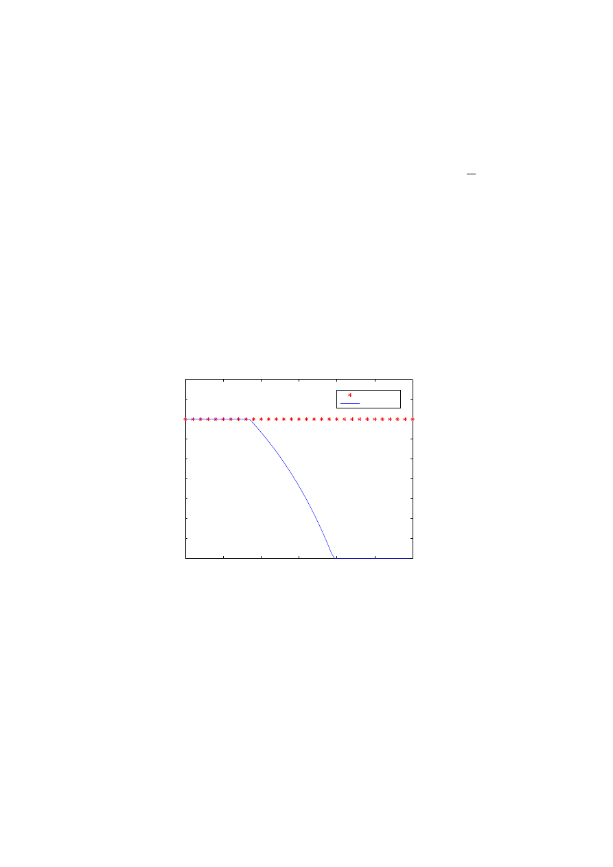
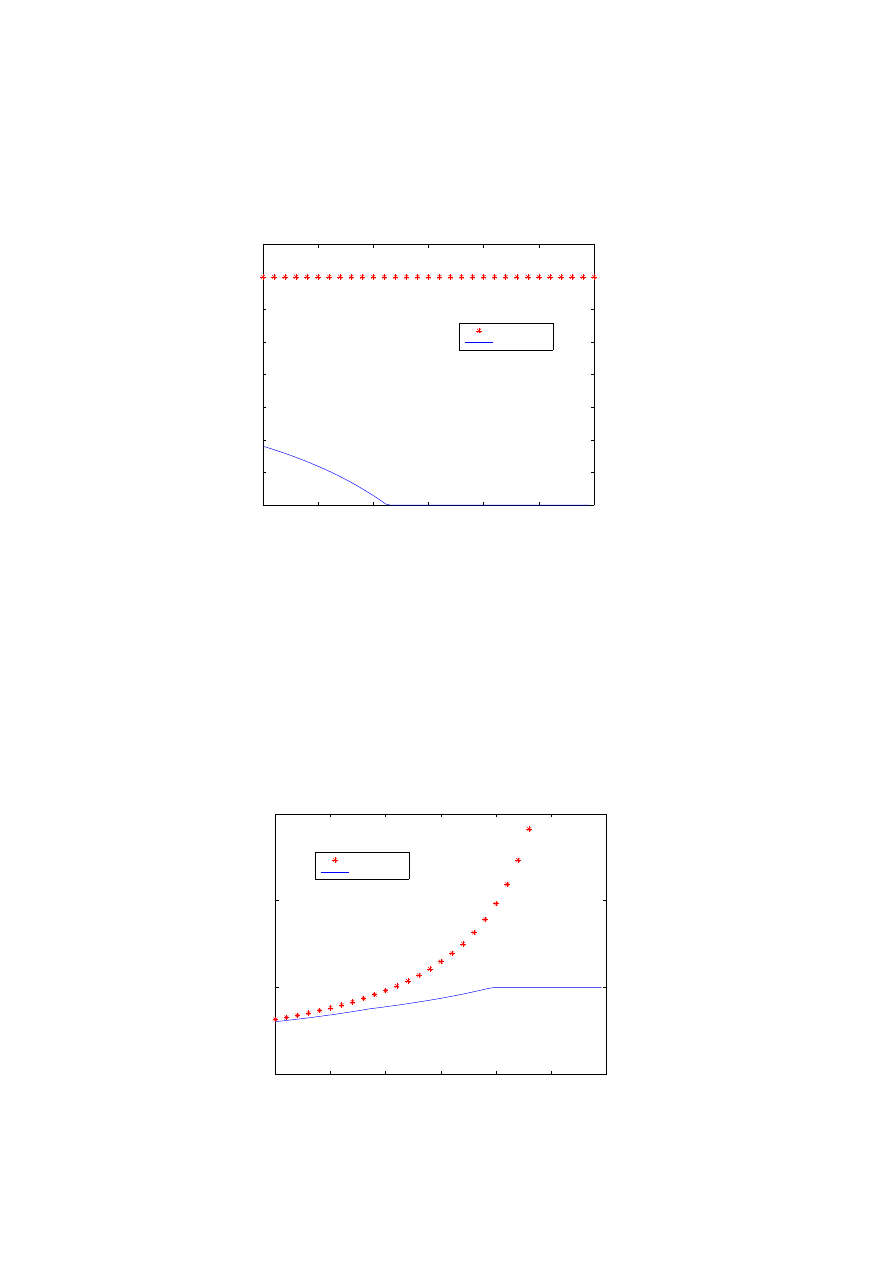
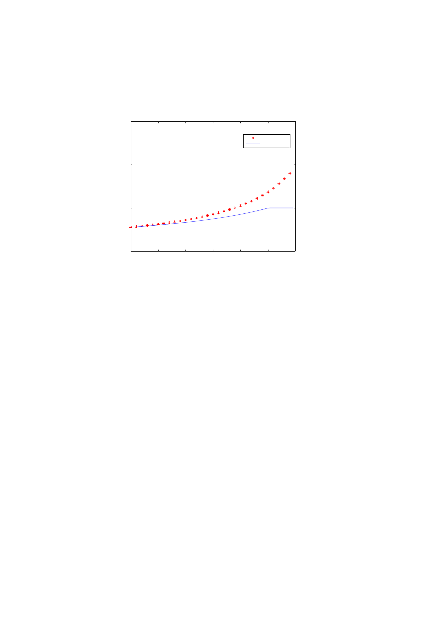
Fig. 1. Asset allocations with and without VaR constraints, for the utility maximizition of
intemporal consumption. The graphs corresponds to different values of CRRA p; p = −1.5,
p = −1, p = −0.5, p = 0, p = 0.5. The x axis represents the time and the y axis the proportion
of wealth invested in stocks. Let us notice the Merton line and, as time goes by the portfolio
value increases hence the VaR constraint becomes binding and reduces the investment in the
risky asset. At the final time the agent is investing the least in stocks (in terms of propor-
tions). When CRRA p increases, i.e., when the agent becomes less risk averse the effect of
VaR constraint becomes more significant.

0.5

1.5

2.5

0.1

0.2

0.3

0.4

0.5

0.6

0.7

0.8

0.9

unconstrained
constrained

0.5

1.5

2.5

0.2

0.4

0.6

0.8

unconstrained
constrained

0.5

1.5

2.5

0.2

0.4

0.6

0.8

1.2

unconstrained
constrained

0.5

1.5

2.5

0.2

0.4

0.6

0.8

1.2

1.4

1.6

1.8

unconstrained
constrained

0.5

1.5

2.5

0.5

1.5

2.5

3.5

unconstrained
constrained

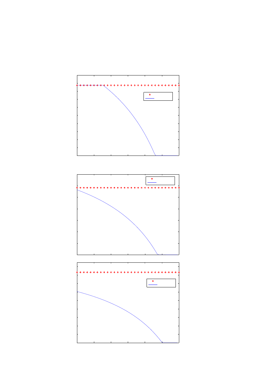
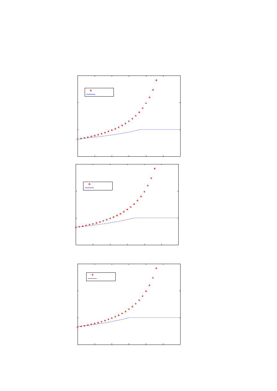
Fig. 2. Asset allocations with and without VaR constraints, for the utility maximizition of
intemporal consumption and terminal wealth. The graphs corresponds to different values of
CRRA p; p = −1.5, p = −1, p = −0.5, p = 0, p = 0.5. The x axis represents the time and the
y axis the proportion of wealth invested in stocks.

0.5

1.5

2.5

0.1

0.2

0.3

0.4

0.5

0.6

0.7

0.8

0.9

unconstrained
constrained

0.5

1.5

2.5

0.1

0.2

0.3

0.4

0.5

0.6

0.7

0.8

0.9

unconstrained
constrained

0.5

1.5

2.5

0.2

0.4

0.6

0.8

1.2

unconstrained
constrained

0.5

1.5

2.5

0.2

0.4

0.6

0.8

1.2

1.4

1.6

1.8

unconstrained
constrained

0.5

1.5

2.5

0.5

1.5

2.5

3.5

unconstrained
constrained

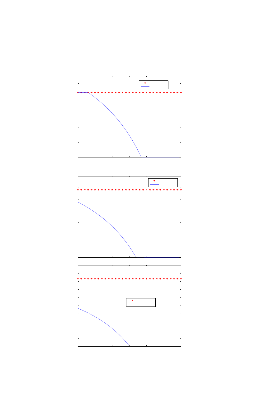
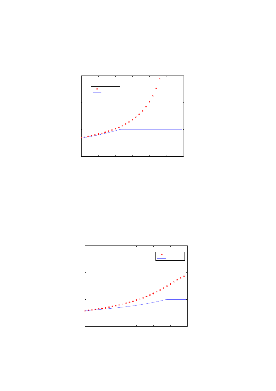
Fig. 3. Optimal consumption with and without VaR constraints, for the utility maximizition
of intemporal consumption. The graphs coresponds to different values of CRRA p; p = −1.5,
p = −1, p = −0.5, p = 0, p = 0.5. The x axis represents the time and the y axis the proportion
of wealth consumed (the expenditure rate). As time goes by, the VaR constraint becomes
active and reduces the consumption (in terms of proportions).

0.5

1.5

2.5

0.5

1.5

unconstrained
constrained

0.5

1.5

2.5

0.5

1.5

unconstrained
constrained

0.5

1.5

2.5

0.5

1.5

unconstrained
constrained

0.5

1.5

2.5

0.5

1.5

unconstrained
constrained

0.5

1.5

2.5

0.5

1.5

unconstrained
constrained

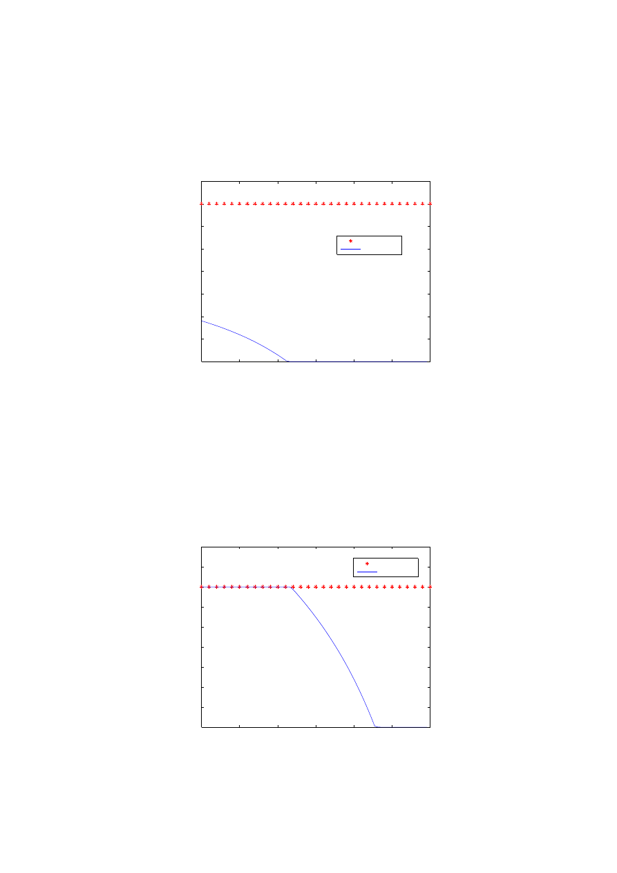
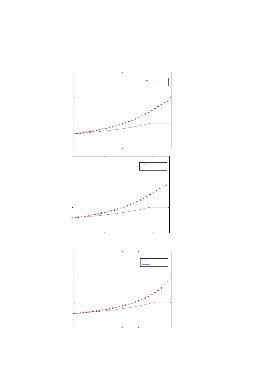
Fig. 4. Optimal consumption with and without VaR constraints, for the utility maxi-

mizition of intemporal consumption and final wealth. The graphs coresponds to different
values of CRRA p; p = −1.5, p = −1, p = −0.5, p = 0, p = 0.5. The x axis represents the time
and the y axis the proportion of wealth consumed (the expenditure rate).

0.5

1.5

2.5

0.5

1.5

unconstrained
constrained

0.5

1.5

2.5

0.5

1.5

unconstrained
constrained

0.5

1.5

2.5

0.5

1.5

unconstrained
constrained

0.5

1.5

2.5

0.5

1.5

unconstrained
constrained

0.5

1.5

2.5

0.5

1.5

unconstrained
constrained

References

[1] Albanese, C. (1997) Credit exposure, Diversification Risk and Coherent VaR, Working

Paper, Department of Mathematics, University of Toronto.

[2] Atkinson, C. and Papakokinou, M. (2005) Theory of optimal consumptionand port-

folio selection under a Capital-at-Risk (CaR) and a Value-at-Risk (VaR) constraint, IMA
Journal of Management Mathematics 16, 37–70.

[3] Basak, S. and Shapiro, A. (2001) Value-at-risk-based risk management: optimal poli-

cies and asset prices, Rev. Financial Studies 14, 371–405.

[4] Berkelaar, A.,Cumperayot P.,Kouwenberg R. (2002) The effect of VaR-based risk

management on asset prices and volatility smile Europen Financial Management 8, 139-
164. 1, 65–78.

[5] Cesari, L. Optimization-theory and applications problems with ordinary differential

equations, Springer-Verlag, New York, 1983.

[6] Cuoco, D., Hua, H. and Issaenko, S. (2001) Optimal dynamic trading strategies with

risk limits, preprint, Yale International Center for Finance.

[7] Cuoco, D. and Liu, H. (2003) An Analysis of VaR-based Capital Requirements,

Preprint, Finance Department, The Wharton School, University of Pennsylvania.

[8] Delbaen F., Schachermayer W. (1994), A general version of the fundamental theorem

of asset pricing , Mathematische Annalen 300, 463-520.

[9] Emmer S., Kl¨

uppelberg and Korn R. (2001), Optimal portfolios with bounded cap-

ital at risk, Mathematical Finance 11, 365-384.

[10] Jorion, P. (1997) Value at Risk, Irwin, Chicago.

[11] Leippold, M., Trojani F. and Vanini P. (2002) Equilibrium impact of value-at-risk,

Preprint, Swiss Banking Institute, University of Zurich, Switzerland.

[12] Karatzas, I. and Shreve, S. E., Brownian Motion and Stochastic Calculus, 2nd Ed.,

Springer-Verlag, New York, 1991.

[13] Merton, R. C. (1969) Lifetime portfolio selection under uncertainty: the continuous-

time case. Rev. Econom. Statist. 51, 247–257.

[14] Merton, R. C. ( 1971) Optimum consumption and portfolio rules in a conitinuous-time

model. J. Economic Theory, 3, 373–413.

[15] Stryk, O (1993) Numerical solution of optimal control problems by direct collocation,

Optimal Control-Calculus of Variations, Optimal Control Theory and Numerical Methods,
International Series of Numerical Mathematics 111, 129–143.

[16] Pirvu, T. A. (2005) Maximizing Portfolio Growth Rate under Risk Constraints, Doctoral

Dissertation, Department of Mathematics, Carnegie Mellon University.

[17] Rivera, J. C. (2004) Portfolio choice under risk limits: a coherent approach, Doctoral

Dissertation, Department of Mathematics, Carnegie Mellon University.

[18] Yiu, K. F. C. (2004) Optimal portfolios under a value-at-risk constraint Journal of

Economic Dynamics& Control 28, 1317-1334.

Wyszukiwarka

Podobne podstrony:
Value at risk
Value at Risk portfel
Value at Risk portfel
Head at risk in LCP
Whos at Risk
Helen Shelton Heart at Risk [MMED 924] (v0 9) (docx) 2
Developing a screening instrument and at risk profile of NSSI behaviour in college women and men
Jaekle Urban, Tomasini Emlio Trading Systems A New Approach To System Development And Portfolio Opt
3 T Proton MRS Investigation of Glutamate and Glutamine in Adolescents at High Genetic Risk for Schi
Prospect theory an analysis of decision under risk
Portfolio Risk Reduction
A Cebenoyan Risk Management, capital structure and lending at banks Journal of banking & finance v
Sexual harassment over the telephone occupational risk at call centres
At the Risk of Forgetting A M Wilson
PORTFOLIO DESIGN AND OPTIMIZATION USING NEURAL NETWORK BASED MULTIAGENT SYSTEM OF INVESTING AGENTS
PIENINY kRoscienko under constr

więcej podobnych podstron