FIRST PAGES
(b) f
/(Nx) = f/(69 · 10) = f/690
Eq. (20-9)
¯x =
8480
69
= 122.9 kcycles
Eq. (20-10)
s
x
=
1 104 600
− 8480
2
/69
69
− 1
1
/
2
= 30.3 kcycles Ans.
x
f
f x
f x
2
f
/(Nx)
60
2
120
7200
0.0029
70
1
70
4900
0.0015
80
3
240
19 200
0.0043
90
5
450
40 500
0.0072
100
8
800
80 000
0.0116
110
12
1320
145 200
0.0174
120
6
720
86 400
0.0087
130
10
1300
169 000
0.0145
140
8
1120
156 800
0.0116
150
5
750
112 500
0.0174
160
2
320
51 200
0.0029
170
3
510
86 700
0.0043
180
2
360
64 800
0.0029
190
1
190
36 100
0.0015
200
0
0
0
0
210
1
210
44 100
0.0015
69
8480
1 104 600
Chapter 20
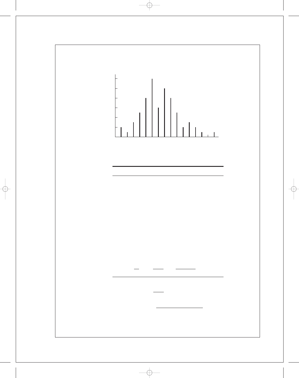
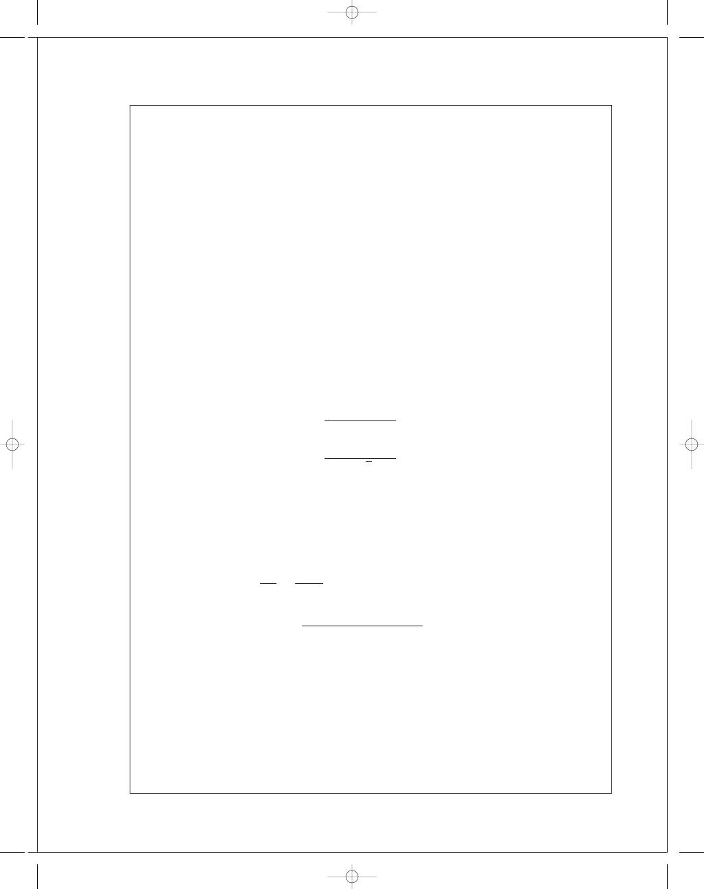
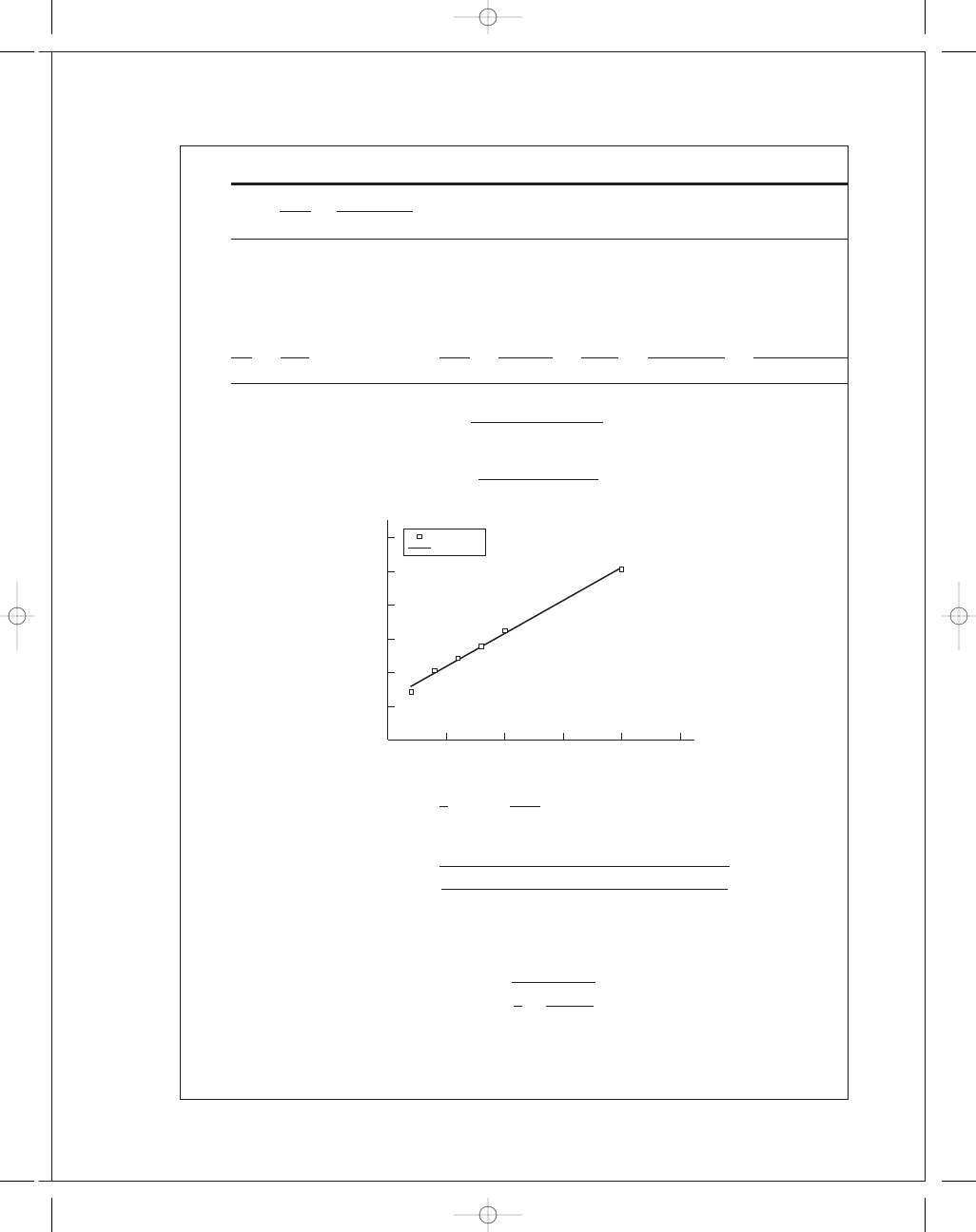
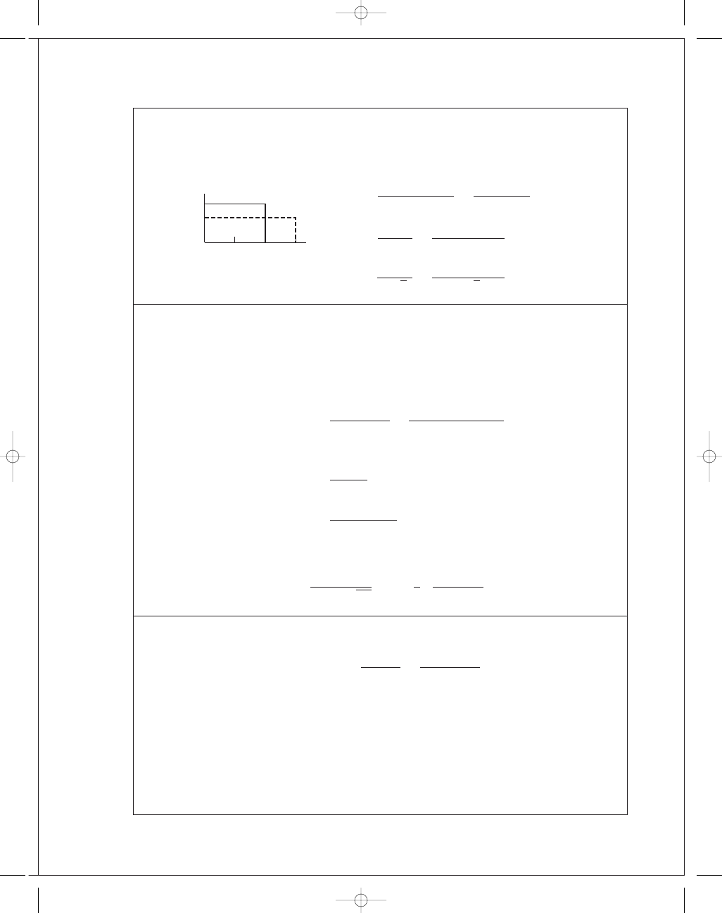
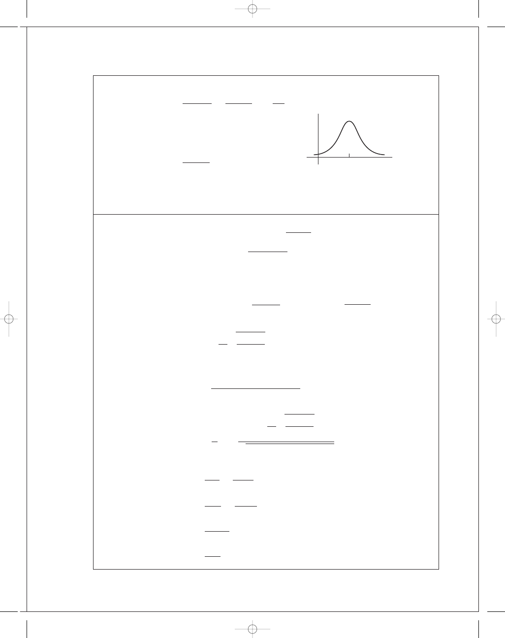
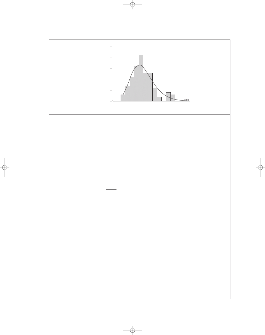
20-1
(a)
0
60
210
190 200
180
170
160
150
140
130
120
110
100
90
80
70
2
4
6
8
10
12
budynas_SM_ch20.qxd 12/06/2006 18:53 Page 1
FIRST PAGES
2
Solutions Manual • Instructor’s Solution Manual to Accompany Mechanical Engineering Design
20-2
Data represents a 7-class histogram with N
= 197.
20-3
Form a table:
¯x =
4548
58
= 78.4 kpsi
s
x
=
359 088
− 4548
2
/58
58
− 1
1
/
2
= 6.57 kpsi
From Eq. (20-14)
f (x)
=
1
6
.57
√
2
π
exp
−
1
2
x
− 78.4
6
.57
2
x
f
f x
f x
2
64
2
128
8192
68
6
408
27 744
72
6
432
31 104
76
9
684
51 984
80
19
1520
121 600
84
10
840
70 560
88
4
352
30 976
92
2
184
16 928
58
4548
359 088
x
f
f x
f x
2
174
6
1044
181 656
182
9
1638
298 116
190
44
8360
1 588 400
198
67
13 266
2 626 688
206
53
10 918
2 249 108
214
12
2568
549 552
220
6
1320
290 400
197
39 114
7 789 900
¯x =
39 114
197
= 198.55 kpsi Ans.
s
x
=
7 783 900
− 39 114
2
/197
197
− 1
1
/
2
= 9.55 kpsi Ans.
budynas_SM_ch20.qxd 12/06/2006 18:53 Page 2
FIRST PAGES
Chapter 20
3
20-4 (a)
y
f
f y
f y
2
y
f
/(Nw)
f (y)
g(y)
5.625
1
5.625
31.640 63
5.625
0.072 727
0.001 262
0.000 295
5.875
0
0
0
5.875
0
0.008 586
0.004 088
6.125
0
0
0
6.125
0
0.042 038
0.031 194
6.375
3
19.125
121.9219
6.375
0.218 182
0.148 106
0.140 262
6.625
3
19.875
131.6719
6.625
0.218 182
0.375 493
0.393 667
6.875
6
41.25
283.5938
6.875
0.436 364
0.685 057
0.725 002
7.125
14
99.75
710.7188
7.125
1.018 182
0.899 389
0.915 128
7.375
15
110.625
815.8594
7.375
1.090 909
0.849 697
0.822 462
7.625
10
76.25
581.4063
7.625
0.727 273
0.577 665
0.544 251
7.875
2
15.75
124.0313
7.875
0.145 455
0.282 608
0.273 138
8.125
1
8.125
66.015 63
8.125
0.072 727
0.099 492
0.106 72
55
396.375
2866.859
For a normal distribution,
¯y = 396.375/55 = 7.207,
s
y
=
2866
.859 − (396.375
2
/55)
55
− 1
1
/
2
= 0.4358
f ( y)
=
1
0
.4358
√
2
π
exp
−
1
2
x
− 7.207
0
.4358
2
For a lognormal distribution,
¯x = ln 7.206 818 − ln
√
1
+ 0.060 474
2
= 1.9732,
s
x
= ln
√
1
+ 0.060 474
2
= 0.0604
g( y)
=
1
x(0
.0604)(
√
2
π)
exp
−
1
2
ln x
− 1.9732
0
.0604
2
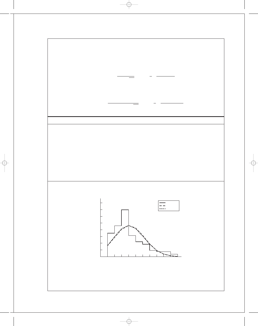
(b) Histogram
0
0.2
0.4
0.6
0.8
1
1.2
5.63
5.88
6.13
6.38
6.63
6.88
log N
7.13
7.38
7.63
7.88
8.13
Data
N
LN
f
budynas_SM_ch20.qxd 12/06/2006 18:53 Page 3
FIRST PAGES
4
Solutions Manual • Instructor’s Solution Manual to Accompany Mechanical Engineering Design
20-5
Distribution is uniform in interval 0.5000 to 0.5008 in, range numbers are a
= 0.5000,
b
= 0.5008 in.
(a) Eq. (20-22)
µ
x
=
a
+ b
2
=
0
.5000 + 0.5008
2
= 0.5004
Eq. (20-23)
σ
x
=
b
− a
2
√
3
=
0
.5008 − 0.5000
2
√
3
= 0.000 231
(b) PDF from Eq. (20-20)
f (x)
=
1250
0
.5000 ≤ x ≤ 0.5008 in
0
otherwise
(c) CDF from Eq. (20-21)
F(x)
=
0
x
< 0.5000
(x
− 0.5)/0.0008 0.5000 ≤ x ≤ 0.5008
1
x
> 0.5008
If all smaller diameters are removed by inspection, a
= 0.5002, b = 0.5008
µ
x
=
0
.5002 + 0.5008
2
= 0.5005 in
ˆσ
x
=
0
.5008 − 0.5002
2
√
3
= 0.000 173 in
f (x)
=
1666
.7 0.5002 ≤ x ≤ 0.5008
0
otherwise
F
(x) =
0
x
< 0.5002
1666
.7(x − 0.5002) 0.5002 ≤ x ≤ 0.5008
1
x
> 0.5008
20-6
Dimensions produced are due to tool dulling and wear. When parts are mixed, the distrib-
ution is uniform. From Eqs. (20-22) and (20-23),
a
= µ
x
−
√
3s
= 0.6241 −
√
3(0
.000 581) = 0.6231 in
b
= µ
x
+
√
3s
= 0.6241 +
√
3(0
.000 581) = 0.6251 in
We suspect the dimension was
0
.623
0
.625
in
Ans.
budynas_SM_ch20.qxd 12/06/2006 18:53 Page 4
FIRST PAGES
Chapter 20
5
20-7
F(x)
= 0.555x − 33 mm
(a) Since F(x) is linear, the distribution is uniform at x
= a
F(a)
= 0 = 0.555(a) − 33
∴ a = 59.46 mm. Therefore, at x = b
F(b)
= 1 = 0.555b − 33
∴ b = 61.26 mm. Therefore,
F(x)
=
0
x
< 59.46 mm
0
.555x − 33 59.46 ≤ x ≤ 61.26 mm
1
x
> 61.26 mm
The PDF is d F
/dx, thus the range numbers are:
f (x)
=
0
.555 59.46 ≤ x ≤ 61.26 mm
0
otherwise
Ans.
From the range numbers,
µ
x
=
59
.46 + 61.26
2
= 60.36 mm Ans.
ˆσ
x
=
61
.26 − 59.46
2
√
3
= 0.520 mm Ans.
1
(b)
σ is an uncorrelated quotient ¯F = 3600 lbf, ¯A = 0.112 in
2
C
F
= 300/3600 = 0.083 33,
C
A
= 0.001/0.112 = 0.008 929
From Table 20-6, for
σ
¯σ =
µ
F
µ
A
=
3600
0
.112
= 32 143 psi Ans.
ˆσ
σ
= 32 143
(0
.08333
2
+ 0.008929
2
)
(1
+ 0.008929
2
)
1
/
2
= 2694 psi Ans.
C
σ
= 2694/32 143 = 0.0838 Ans.
Since F and A are lognormal, division is closed and
σ is lognormal too.
σ = LN(32 143, 2694) psi Ans.
budynas_SM_ch20.qxd 12/06/2006 18:53 Page 5
FIRST PAGES
6
Solutions Manual • Instructor’s Solution Manual to Accompany Mechanical Engineering Design
20-8
Cramer’s rule
a
1
=
y
x
2
xy x
3
x
x
2
x
2
x
3
=
yx
3
− xyx
2
xx
3
− (x
2
)
2
Ans.
a
2
=
x
y
x
2
xy
x
x
2
x
2
x
3
=
xxy − yx
2
xx
3
− (x
2
)
2
Ans.
0.05
0
0.05
0.1
0.15
0.2
0.25
0.3
0
0.2
0.4
0.6
0.8
1
Data
Regression
x
y
x
y
x
2
x
3
xy
0
0.01
0
0
0
0.2
0.15
0.04
0.008
0.030
0.4
0.25
0.16
0.064
0.100
0.6
0.25
0.36
0.216
0.150
0.8
0.17
0.64
0.512
0.136
1.0
−0.01
1.00
1.000
−0.010
3.0
0.82
2.20
1.800
0.406
a
1
= 1.040 714
a
2
= −1.046 43 Ans.
Data
Regression
x
y
y
0
0.01
0
0.2
0.15
0.166 286
0.4
0.25
0.248 857
0.6
0.25
0.247 714
0.8
0.17
0.162 857
1.0
−0.01
−0.005 71
budynas_SM_ch20.qxd 12/06/2006 18:53 Page 6
FIRST PAGES
Chapter 20
7
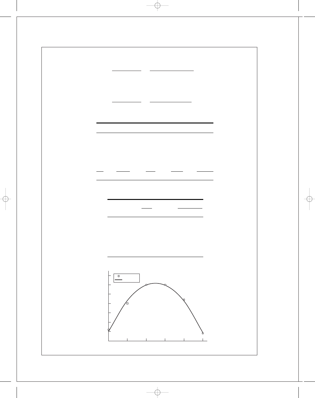
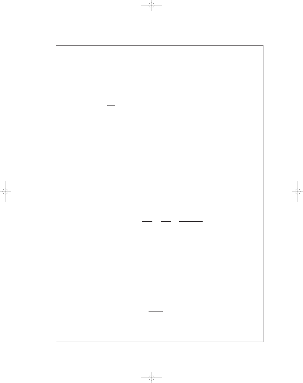
20-9
0
20
40
60
80
100
120
140
0
100
200
S
u
S
e
300
400
Data
Regression
Data
Regression
S
u
S
e
S
e
S
2
u
S
u
S
e
0
20.356 75
60
30
39.080 78
3 600
1 800
64
48
40.329 05
4 096
3 072
65
29.5
40.641 12
4 225
1 917.5
82
45
45.946 26
6 724
3 690
101
51
51.875 54
10 201
5 151
119
50
57.492 75
14 161
5 950
120
48
57.804 81
14 400
5 760
130
67
60.925 48
16 900
8 710
134
60
62.173 75
17 956
8 040
145
64
65.606 49
21 025
9 280
180
84
76.528 84
32 400
15 120
195
78
81.209 85
38 025
15 210
205
96
84.330 52
42 025
19 680
207
87
84.954 66
42 849
18 009
210
87
85.890 86
44 100
18 270
213
75
86.827 06
45 369
15 975
225
99
90.571 87
50 625
22 275
225
87
90.571 87
50 625
19 575
227
116
91.196
51 529
26 332
230
105
92.132 2
52 900
24 150
238
109
94.628 74
56 644
25 942
242
106
95.877 01
58 564
25 652
265
105
103.054 6
70 225
27 825
280
96
107.735 6
78 400
26 880
295
99
112.416 6
87 025
29 205
325
114
121.778 6
105 625
37 050
325
117
121.778 6
105 625
38 025
355
122
131.140 6
126 025
43 310
5462
2274.5
1 251 868
501 855.5
m
= 0.312067
b
= 20.35675 Ans.
budynas_SM_ch20.qxd 12/06/2006 18:53 Page 7
FIRST PAGES
8
Solutions Manual • Instructor’s Solution Manual to Accompany Mechanical Engineering Design
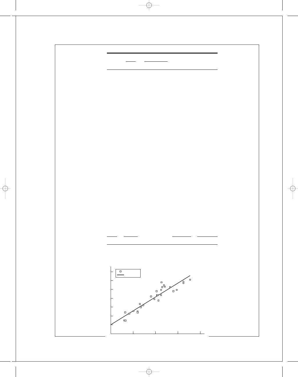
20-10
E
=
y
− a
0
− a
2
x
2
2
∂
E
∂a
0
= −2
y
− a
0
− a
2
x
2
= 0
y
− na
0
− a
2
x
2
= 0 ⇒
y
= na
0
+ a
2
x
2
∂
E
∂a
2
= 2
y
− a
0
− a
2
x
2
(2x)
= 0 ⇒
x y
= a
0
x
+ a
2
x
3
Ans.
Cramer’s rule
a
0
=
y
x
2
xy x
3
n
x
2
x x
3
=
x
3
y − x
2
xy
n
x
3
− xx
2
a
2
=
n
y
x xy
n
x
2
x x
3
=
n
xy − xy
n
x
3
− xx
2
a
0
=
800 000(56)
− 12 000(2400)
4(800 000)
− 200(12 000)
= 20
a
2
=
4(2400)
− 200(56)
4(800 000)
− 200(12 000)
= −0.002
Data
Regression
0
5
10
15
y
x
20
25
0
20
40
60
80
100
Data
Regression
x
y
y
x
2
x
3
xy
20
19
19.2
400
8 000
380
40
17
16.8
1600
64 000
680
60
13
12.8
3600
216 000
780
80
7
7.2
6400
512 000
560
200
56
12 000
800 000
2400
budynas_SM_ch20.qxd 12/06/2006 18:53 Page 8
FIRST PAGES
Chapter 20
9
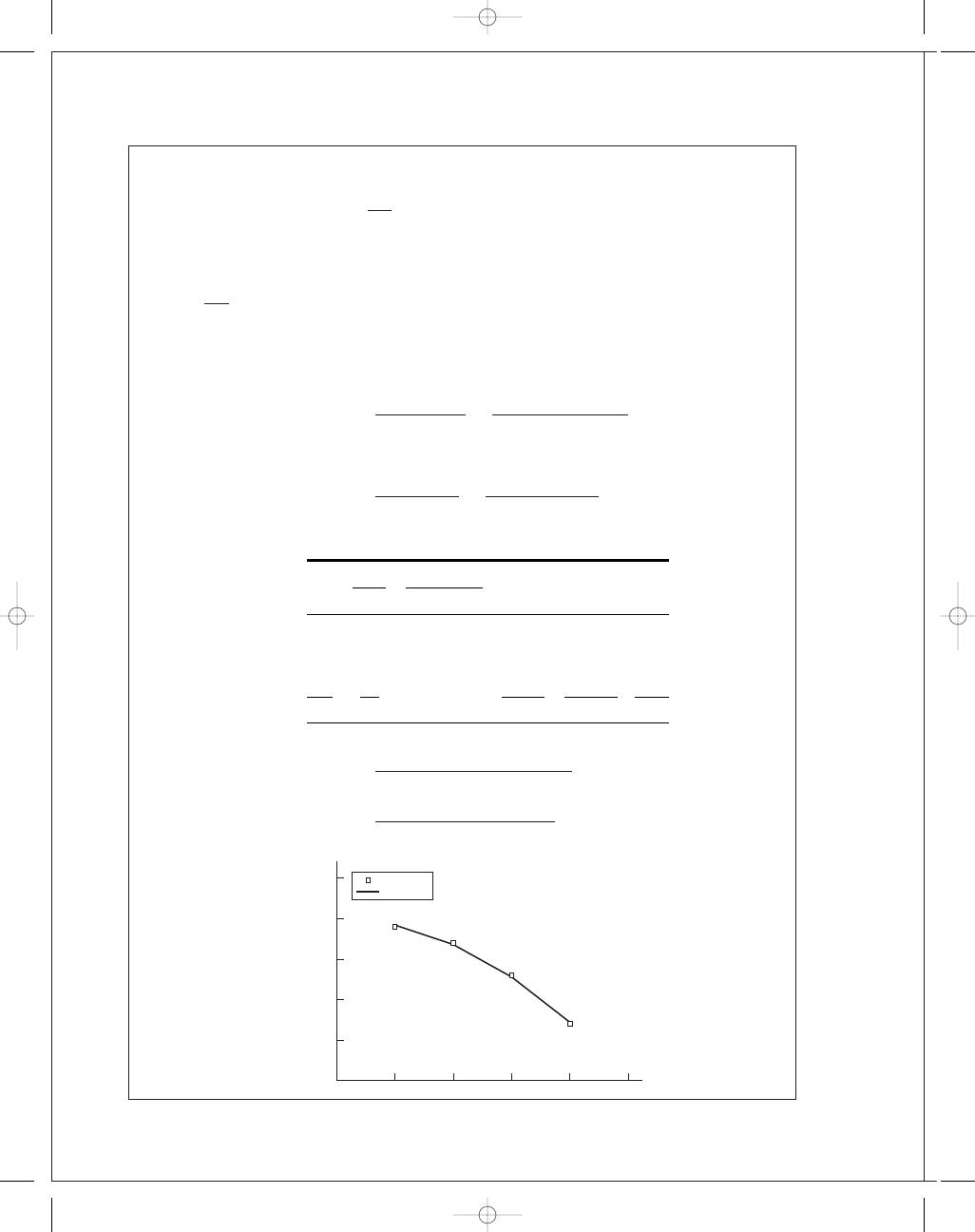
20-11
Data
Regression
x
y
y
x
2
y
2
x y
x
− ¯x
(x
− ¯x)
2
0.2
7.1
7.931 803
0.04
50.41
1.42
−0.633333
0.401 111 111
0.4
10.3
9.884 918
0.16
106.09
4.12
−0.433333
0.187 777 778
0.6
12.1
11.838 032
0.36
146.41
7.26
−0.233333
0.054 444 444
0.8
13.8
13.791 147
0.64
190.44
11.04
−0.033333
0.001 111 111
1
16.2
15.744 262
1.00
262.44
16.20
0.166 666
0.027 777 778
2
25.2
25.509 836
4.00
635.04
50.40
1.166 666
1.361 111 111
5
84.7
6.2
1390.83
90.44
0
2.033 333 333
ˆm = ¯k =
6(90
.44) − 5(84.7)
6(6
.2) − (5)
2
= 9.7656
ˆb = ¯F
i
=
84
.7 − 9.7656(5)
6
= 5.9787
(a)
¯x =
5
6
;
¯y =
84
.7
6
= 14.117
Eq. (20-37)
s
yx
=
1390
.83 − 5.9787(84.7) − 9.7656(90.44)
6
− 2
= 0.556
Eq. (20-36)
s
ˆb
= 0.556
1
6
+
(5
/6)
2
2
.0333
= 0.3964 lbf
F
i
= (5.9787, 0.3964) lbf Ans.
F
x
0
5
10
15
20
25
30
0
1
0.5
1.5
2
2.5
Data
Regression
budynas_SM_ch20.qxd 12/06/2006 18:53 Page 9
FIRST PAGES
(b) Eq. (20-35)
s
ˆm
=
0
.556
√
2
.0333
= 0.3899 lbf/in
k
= (9.7656, 0.3899) lbf/in Ans.
20-12 The expression
= δ/l is of the form x/y. Now δ = (0.0015, 0.000 092) in, unspecified
distribution; l
= (2.000, 0.0081) in, unspecified distribution;
C
x
= 0.000 092/0.0015 = 0.0613
C
y
= 0.0081/2.000 = 0.000 75
From Table 20-6,
¯ = 0.0015/2.000 = 0.000 75
ˆσ
= 0.000 75
0
.0613
2
+ 0.004 05
2
1
+ 0.004 05
2
1
/
2
= 4.607(10
−5
) = 0.000 046
We can predict
¯ and ˆσ
but not the distribution of
.
20-13
σ = E
= (0.0005, 0.000 034) distribution unspecified; E = (29.5, 0.885) Mpsi, distribution
unspecified;
C
x
= 0.000 034/0.0005 = 0.068,
C
y
= 0.0885/29.5 = 0.030
σ is of the form x, y
Table 20-6
¯σ = ¯ ¯E = 0.0005(29.5)10
6
= 14 750 psi
ˆσ
σ
= 14 750(0.068
2
+ 0.030
2
+ 0.068
2
+ 0.030
2
)
1
/
2
= 1096.7 psi
C
σ
= 1096.7/14 750 = 0.074 35
20-14
δ =
Fl
AE
F
= (14.7, 1.3) kip, A = (0.226, 0.003) in
2
, l
= (1.5, 0.004) in, E = (29.5, 0.885) Mpsi dis-
tributions unspecified.
C
F
= 1.3/14.7 = 0.0884; C
A
= 0.003/0.226 = 0.0133; C
l
= 0.004/1.5 = 0.00267;
C
E
= 0.885/29.5 = 0.03
Mean of
δ:
δ =
Fl
AE
= Fl
1
A
1
E
10
Solutions Manual • Instructor’s Solution Manual to Accompany Mechanical Engineering Design
budynas_SM_ch20.qxd 12/06/2006 18:53 Page 10
FIRST PAGES
Chapter 20
11
From Table 20-6,
¯δ = ¯F ¯l(1/ ¯A)(1/ ¯E)
¯δ = 14 700(1.5)
1
0
.226
1
29
.5(10
6
)
= 0.003 31 in Ans.
For the standard deviation, using the first-order terms in Table 20-6,
ˆσ
δ
.= ¯F¯l
¯A ¯E
C
2
F
+ C
2
l
+ C
2
A
+ C
2
E
1
/
2
= ¯δ
C
2
F
+ C
2
l
+ C
2
A
+ C
2
E
1
/
2
ˆσ
δ
= 0.003 31(0.0884
2
+ 0.00267
2
+ 0.0133
2
+ 0.03
2
)
1
/
2
= 0.000 313 in Ans.
COV
C
δ
= 0.000 313/0.003 31 = 0.0945 Ans.
Force COV dominates. There is no distributional information on
δ.
20-15 M
= (15000, 1350) lbf · in, distribution unspecified; d = (2.00, 0.005) in distribution
unspecified.
σ =
32M
πd
3
,
C
M
=
1350
15 000
= 0.09, C
d
=
0
.005
2
.00
= 0.0025
σ is of the form x/y, Table 20-6.
Mean:
¯σ =
32 ¯
M
π
d
3
.= 32 ¯M
π ¯d
3
=
32(15 000)
π(2
3
)
= 19 099 psi Ans.
Standard Deviation:
ˆσ
σ
= ¯σ
C
2
M
+ C
2
d
3
1
+ C
2
d
3
1
/
2
From Table 20-6,
C
d
3
.= 3C
d
= 3(0.0025) = 0.0075
ˆσ
σ
= ¯σ
C
2
M
+ (3C
d
)
2
(1
+ (3C
d
))
2
1
/
2
= 19 099[(0.09
2
+ 0.0075
2
)/(1 + 0.0075
2
)]
1
/2
= 1725 psi Ans.
COV:
C
σ
=
1725
19 099
= 0.0903 Ans.
Stress COV dominates. No information of distribution of
σ.
budynas_SM_ch20.qxd 12/06/2006 18:53 Page 11
FIRST PAGES
12
Solutions Manual • Instructor’s Solution Manual to Accompany Mechanical Engineering Design
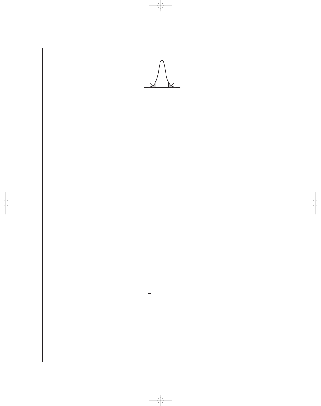
20-16
Fraction discarded is
α + β. The area under the PDF was unity. Having discarded α + β
fraction, the ordinates to the truncated PDF are multiplied by a.
a
=
1
1
− (α + β)
New PDF, g(x) , is given by
g
(x) =
f
(x)/[1 − (α + β)] x
1
≤ x ≤ x
2
0
otherwise
More formal proof: g
(x) has the property
1
=
x
2
x
1
g
(x) dx = a
x
2
x
1
f
(x) dx
1
= a
∞
−∞
f
(x) dx −
x
1
0
f
(x) dx −
∞
x
2
f
(x) dx
1
= a {1 − F(x
1
) − [1 − F(x
2
)]}
a
=
1
F(x
2
)
− F(x
1
)
=
1
(1
− β) − α
=
1
1
− (α + β)
20-17
(a) d
= U[0.748, 0.751]
µ
d
=
0
.751 + 0.748
2
= 0.7495 in
ˆσ
d
=
0
.751 − 0.748
2
√
3
= 0.000 866 in
f (x)
=
1
b
− a
=
1
0
.751 − 0.748
= 333.3 in
−
1
F(x)
=
x
− 0.748
0
.751 − 0.748
= 333.3(x − 0.748)
x
1
f (x)
x
x
2
␣

budynas_SM_ch20.qxd 12/06/2006 18:53 Page 12
FIRST PAGES
Chapter 20
13
(b)
F(x
1
)
= F(0.748) = 0
F(x
2
)
= (0.750 − 0.748)333.3 = 0.6667
If g
(x) is truncated, PDF becomes
g(x)
=
f (x)
F(x
2
)
− F(x
1
)
=
333
.3
0
.6667 − 0
= 500 in
−
1
µ
x
=
a
+ b
2
=
0
.748 + 0.750
2
= 0.749 in
ˆσ
x
=
b
− a
2
√
3
=
0
.750 − 0.748
2
√
3
= 0.000 577 in
20-18
From Table A-10, 8.1% corresponds to z
1
= −1.4 and 5.5% corresponds to z
2
= +1.6.
k
1
= µ + z
1
ˆσ
k
2
= µ + z
2
ˆσ
From which
µ =
z
2
k
1
− z
1
k
2
z
2
− z
1
=
1
.6(9) − (−1.4)11
1
.6 − (−1.4)
= 9.933
ˆσ =
k
2
− k
1
z
2
− z
1
=
11
− 9
1
.6 − (−1.4)
= 0.6667
The original density function is
f (k)
=
1
0
.6667
√
2
π
exp
−
1
2
k
− 9.933
0
.6667
2
Ans.
20-19
From Prob. 20-1,
µ = 122.9 kcycles and ˆσ = 30.3 kcycles.
z
10
=
x
10
− µ
ˆσ
=
x
10
− 122.9
30
.3
x
10
= 122.9 + 30.3z
10
From Table A-10, for 10 percent failure, z
10
= −1.282
x
10
= 122.9 + 30.3(−1.282)
= 84.1 kcycles Ans.
0.748
g(x)
500
x
f (x)
333.3
0.749
0.750
0.751
budynas_SM_ch20.qxd 12/06/2006 18:53 Page 13
FIRST PAGES
14
Solutions Manual • Instructor’s Solution Manual to Accompany Mechanical Engineering Design
20-20
x
f
f x
f x
2
x
f
/(Nw)
f (x)
60
2
120
7200
60
0.002 899
0.000 399
70
1
70
4900
70
0.001 449
0.001 206
80
3
240
19 200
80
0.004 348
0.003 009
90
5
450
40 500
90
0.007 246
0.006 204
100
8
800
80 000
100
0.011 594
0.010 567
110
12
1320
145 200
110
0.017 391
0.014 871
120
6
720
86 400
120
0.008 696
0.017 292
130
10
1300
169 000
130
0.014 493
0.016 612
140
8
1120
156 800
140
0.011 594
0.013 185
150
5
750
112 500
150
0.007 246
0.008 647
160
2
320
51 200
160
0.002 899
0.004 685
170
3
510
86 700
170
0.004 348
0.002 097
180
2
360
64 800
180
0.002 899
0.000 776
190
1
190
36 100
190
0.001 449
0.000 237
200
0
0
0
200
0
5.98E-05
210
1
210
44 100
210
0.001 449
1.25E-05
69
8480
¯x = 122.8986
s
x
= 22.88719
x
f
/(Nw)
f (x)
x
f
/(Nw)
f (x)
55
0
0.000 214
145
0.011 594
0.010 935
55
0.002 899
0.000 214
145
0.007 246
0.010 935
65
0.002 899
0.000 711
155
0.007 246
0.006 518
65
0.001 449
0.000 711
155
0.002 899
0.006 518
75
0.001 449
0.001 951
165
0.002 899
0.003 21
75
0.004 348
0.001 951
165
0.004 348
0.003 21
85
0.004 348
0.004 425
175
0.004 348
0.001 306
85
0.007 246
0.004 425
175
0.002 899
0.001 306
95
0.007 246
0.008 292
185
0.002 899
0.000 439
95
0.011 594
0.008 292
185
0.001 449
0.000 439
105
0.011 594
0.012 839
195
0.001 449
0.000 122
105
0.017 391
0.012 839
195
0
0.000 122
115
0.017 391
0.016 423
205
0
2.8E-05
115
0.008 696
0.016 423
205
0.001 499
2.8E-05
125
0.008 696
0.017 357
215
0.001 499
5.31E-06
125
0.014 493
0.017 357
215
0
5.31E-06
135
0.014 493
0.015 157
135
0.011 594
0.015 157
budynas_SM_ch20.qxd 12/06/2006 18:53 Page 14
FIRST PAGES
Chapter 20
15
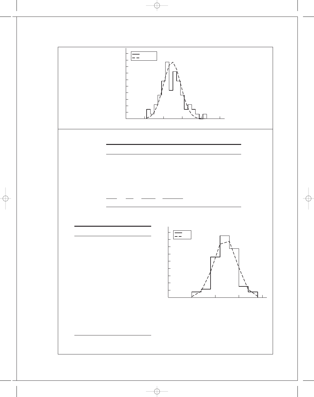
20-21
x
f
f x
f x
2
f
/(Nw)
f (x)
174
6
1044
181 656
0.003 807
0.001 642
182
9
1638
298 116
0.005 711
0.009 485
190
44
8360
1 588 400
0.027 919
0.027 742
198
67
13 266
2 626 668
0.042 513
0.041 068
206
53
10 918
2 249 108
0.033 629
0.030 773
214
12
2568
549 552
0.007 614
0.011 671
222
6
1332
295 704
0.003 807
0.002 241
1386
197
39 126
7 789 204
¯x = 198.6091
s
x
= 9.695071
x
f
/(Nw)
f (x)
170
0
0.000 529
170
0.003 807
0.000 529
178
0.003 807
0.004 297
178
0.005 711
0.004 297
186
0.005 711
0.017 663
186
0.027 919
0.017 663
194
0.027 919
0.036 752
194
0.042 513
0.036 752
202
0.042 513
0.038 708
202
0.033 629
0.038 708
210
0.033 629
0.020 635
210
0.007 614
0.020 635
218
0.007 614
0.005 568
218
0.003 807
0.005 568
226
0.003 807
0.000 76
226
0
0.000 76
Data
PDF
0
0.005
0.01
0.015
0.02
0.025
0.03
0.035
0.04
0.045
150
170
190
210
x
230
f
Histogram
PDF
0
0.002
0.004
0.006
0.008
0.01
0.012
0.014
0.016
0.018
f
x
0.02
0
50
100
150
200
250
budynas_SM_ch20.qxd 12/06/2006 18:53 Page 15
FIRST PAGES
16
Solutions Manual • Instructor’s Solution Manual to Accompany Mechanical Engineering Design
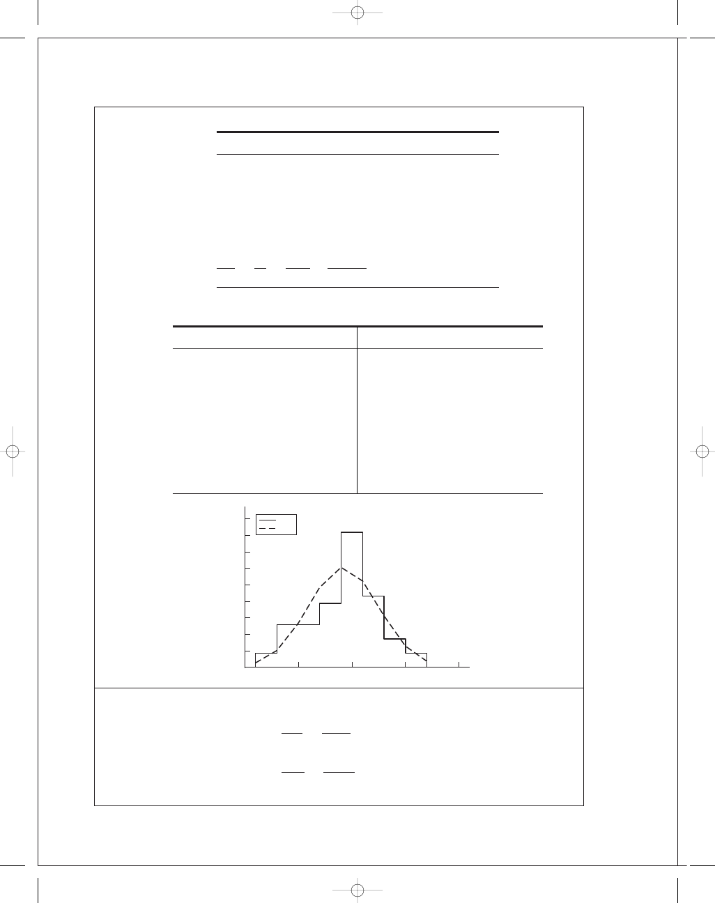
20-22
x
f
f x
f x
2
f
/(Nw)
f (x)
64
2
128
8192
0.008 621
0.005 48
68
6
408
27 744
0.025 862
0.017 299
72
6
432
31 104
0.025 862
0.037 705
76
9
684
51 984
0.038 793
0.056 742
80
19
1520
121 600
0.081 897
0.058 959
84
10
840
70 560
0.043 103
0.042 298
88
4
352
30 976
0.017 241
0.020 952
92
2
184
16 928
0.008 621
0.007 165
624
58
4548
359 088
¯x = 78.41379
s
x
= 6.572229
x
f
/(Nw)
f (x)
x
f
/(Nw)
f (x)
62
0
0.002 684
82
0.081 897
0.052 305
62
0.008 621
0.002 684
82
0.043 103
0.052 305
66
0.008 621
0.010 197
86
0.043 103
0.031 18
66
0.025 862
0.010 197
86
0.017 241
0.031 18
70
0.025 862
0.026 749
90
0.017 241
0.012 833
70
0.025 862
0.026 749
90
0.008 621
0.012 833
74
0.025 862
0.048 446
94
0.008 621
0.003 647
74
0.038 793
0.048 446
94
0
0.003 647
78
0.038 793
0.060 581
78
0.081 897
0.060 581
20-23
¯σ =
4 ¯
P
πd
2
=
4(40)
π(1
2
)
= 50.93 kpsi
ˆσ
σ
=
4
ˆσ
P
πd
2
=
4(8
.5)
π(1
2
)
= 10.82 kpsi
ˆσ
s
y
= 5.9 kpsi
Data
PDF
x
0
0.01
0.02
0.03
0.04
0.05
0.06
0.07
0.08
0.09
60
70
80
90
100
f
budynas_SM_ch20.qxd 12/06/2006 18:53 Page 16
FIRST PAGES
Chapter 20
17
For no yield, m
= S
y
− σ ≥ 0
z
=
m
− µ
m
ˆσ
m
=
0
− µ
m
ˆσ
m
= −
µ
m
ˆσ
m
µ
m
= ¯S
y
− ¯σ = 27.47 kpsi,
ˆσ
m
=
ˆσ
2
σ
+ ˆσ
2
S
y
1
/
2
= 12.32 kpsi
z
=
−27.47
12
.32
= −2.230
From Table A-10, p
f
= 0.0129
R
= 1 − p
f
= 1 − 0.0129 = 0.987 Ans.
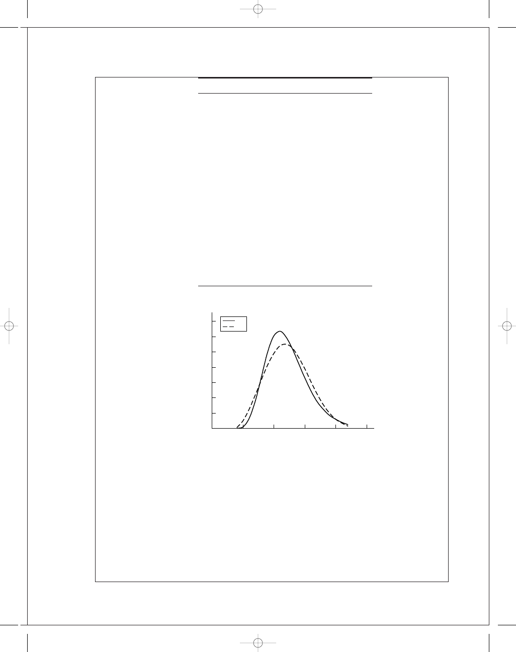
20-24 For a lognormal distribution,
Eq. (20-18)
µ
y
= ln µ
x
− ln
1
+ C
2
x
Eq. (20-19)
ˆσ
y
=
ln
1
+ C
2
x
From Prob. (20-23)
µ
m
= ¯S
y
− ¯σ = µ
x
µ
y
=
ln ¯
S
y
− ln
1
+ C
2
S
y
−
ln
¯σ − ln
1
+ C
2
σ
= ln
¯S
y
¯σ
1
+ C
2
σ
1
+ C
2
S
y
ˆσ
y
=
ln
1
+ C
2
S
y
+ ln
1
+ C
2
σ
1
/
2
=
ln
1
+ C
2
S
y
1
+ C
2
σ
z
= −
µ
ˆσ
= −
ln
¯S
y
¯σ
1
+ C
2
σ
1
+ C
2
S
y
ln
1
+ C
2
S
y
1
+ C
2
σ
¯σ =
4 ¯
P
πd
2
=
4(30)
π(1
2
)
= 38.197 kpsi
ˆσ
σ
=
4
ˆσ
P
πd
2
=
4(5
.1)
π(1
2
)
= 6.494 kpsi
C
σ
=
6
.494
38
.197
= 0.1700
C
S
y
=
3
.81
49
.6
= 0.076 81
0
m
budynas_SM_ch20.qxd 12/06/2006 18:53 Page 17
FIRST PAGES
18
Solutions Manual • Instructor’s Solution Manual to Accompany Mechanical Engineering Design
z
= −
ln
49.6
38
.197
1
+ 0.170
2
1
+ 0.076 81
2
ln
(1
+ 0.076 81
2
)(1
+ 0.170
2
)
= −1.470
From Table A-10
p
f
= 0.0708
R
= 1 − p
f
= 0.929 Ans.
20-25
x
n
n x
nx
2
93
19
1767
164 311
95
25
2375
225 625
97
38
3685
357 542
99
17
1683
166 617
101
12
1212
122 412
103
10
1030
106 090
105
5
525
55 125
107
4
428
45 796
109
4
436
47 524
111
2
222
24 624
136
13 364
1315 704
¯x = 13 364/136 = 98.26 kpsi
s
x
=
1 315 704
− 13 364
2
/136
135
1
/
2
= 4.30 kpsi
Under normal hypothesis,
z
0
.
01
= (x
0
.
01
− 98.26)/4.30
x
0
.
01
= 98.26 + 4.30z
0
.
01
= 98.26 + 4.30(−2.3267)
= 88.26 .= 88.3 kpsi Ans.
20-26 From Prob. 20-25,
µ
x
= 98.26 kpsi, and ˆσ
x
= 4.30 kpsi.
C
x
= ˆσ
x
/µ
x
= 4.30/98.26 = 0.043 76
From Eqs. (20-18) and (20-19),
µ
y
= ln(98.26) − 0.043 76
2
/2 = 4.587
ˆσ
y
=
!
ln(1
+ 0.043 76
2
)
= 0.043 74
For a yield strength exceeded by 99% of the population,
z
0
.
01
= (ln x
0
.
01
− µ
y
)
/ ˆσ
y
⇒ ln x
0
.
01
= µ
y
+ ˆσ
y
z
0
.
01
budynas_SM_ch20.qxd 12/06/2006 18:53 Page 18
FIRST PAGES
Chapter 20
19
From Table A-10, for 1% failure, z
0
.
01
= −2.326. Thus,
ln x
0
.
01
= 4.587 + 0.043 74(−2.326) = 4.485
x
0
.
01
= 88.7 kpsi Ans.
The normal PDF is given by Eq. (20-14) as
f (x)
=
1
4
.30
√
2
π
exp
−
1
2
x
− 98.26
4
.30
2
For the lognormal distribution, from Eq. (20-17), defining g(x),
g(x)
=
1
x(0
.043 74)
√
2
π
exp
−
1
2
ln x
− 4.587
0
.043 74
2
x (kpsi)
f
/(Nw)
f (x)
g (x)
x (kpsi)
f
/(Nw)
f (x)
g (x)
92
0.000 00
0.032 15
0.032 63
102
0.036 76
0.063 56
0.061 34
92
0.069 85
0.032 15
0.032 63
104
0.036 76
0.038 06
0.037 08
94
0.069 85
0.056 80
0.058 90
104
0.018 38
0.038 06
0.037 08
94
0.091 91
0.056 80
0.058 90
106
0.018 38
0.018 36
0.018 69
96
0.091 91
0.080 81
0.083 08
106
0.014 71
0.018 36
0.018 69
96
0.139 71
0.080 81
0.083 08
108
0.014 71
0.007 13
0.007 93
98
0.139 71
0.092 61
0.092 97
108
0.014 71
0.007 13
0.007 93
98
0.062 50
0.092 61
0.092 97
110
0.014 71
0.002 23
0.002 86
100
0.062 50
0.085 48
0.083 67
110
0.007 35
0.002 23
0.002 86
100
0.044 12
0.085 48
0.083 67
112
0.007 35
0.000 56
0.000 89
102
0.044 12
0.063 56
0.061 34
112
0.000 00
0.000 56
0.000 89
Note: rows are repeated to draw histogram
The normal and lognormal are almost the same. However the data is quite skewed and
perhaps a Weibull distribution should be explored. For a method of establishing the
f (x)
g(x)
Histogram
0
0.02
0.04
0.06
0.08
0.1
0.12
0.14
0.16
90
92
94
96
98
100
102
104
106
108
x (kpsi)
Probability density
110
112
budynas_SM_ch20.qxd 12/06/2006 18:53 Page 19
FIRST PAGES
20
Solutions Manual • Instructor’s Solution Manual to Accompany Mechanical Engineering Design
Weibull parameters see Shigley, J. E., and C. R. Mischke, Mechanical Engineering Design,
McGraw-Hill, 5th ed., 1989, Sec. 4-12.
20-27 Let x
= (S
f e
)
10
4
x
0
= 79 kpsi, θ = 86.2 kpsi, b = 2.6
Eq. (20-28)
¯x = x
0
+ (θ − x
0
)
(1 + 1/b)
¯x = 79 + (86.2 − 79)(1 + 1/2.6)
= 79 + 7.2 (1.38)
From Table A-34,
(1.38) = 0.88854
¯x = 79 + 7.2(0.888 54) = 85.4 kpsi Ans.
Eq. (20-29)
ˆσ
x
= (θ − x
0
)[
(1 + 2/b) −
2
(1
+ 1/b)]
1
/
2
= (86.2 − 79)[(1 + 2/2.6) −
2
(1
+ 1/2.6)]
1
/
2
= 7.2[0.923 76 − 0.888 54
2
]
1
/
2
= 2.64 kpsi Ans.
C
x
=
ˆσ
x
¯x
=
2
.64
85
.4
= 0.031 Ans.
20-28
x
= S
ut
x
0
= 27.7, θ = 46.2, b = 4.38
µ
x
= 27.7 + (46.2 − 27.7)(1 + 1/4.38)
= 27.7 + 18.5 (1.23)
= 27.7 + 18.5(0.910 75)
= 44.55 kpsi Ans.
ˆσ
x
= (46.2 − 27.7)[(1 + 2/4.38) −
2
(1
+ 1/4.38)]
1
/
2
= 18.5[(1.46) −
2
(1
.23)]
1
/
2
= 18.5[0.8856 − 0.910 75
2
]
1
/
2
= 4.38 kpsi Ans.
C
x
=
4
.38
44
.55
= 0.098 Ans.
From the Weibull survival equation
R
= exp
−
x
− x
0
θ − x
0
b
= 1 − p
budynas_SM_ch20.qxd 12/06/2006 19:32 Page 20
FIRST PAGES
Chapter 20
21
R
40
= exp
−
x
40
− x
0
θ − x
0
b
= 1 − p
40
= exp
−
40
− 27.7
46
.2 − 27.7
4
.
38
= 0.846
p
40
= 1 − R
40
= 1 − 0.846 = 0.154 = 15.4% Ans.
20-29
x
= S
ut
x
0
= 151.9, θ = 193.6, b = 8
µ
x
= 151.9 + (193.6 − 151.9)(1 + 1/8)
= 151.9 + 41.7 (1.125)
= 151.9 + 41.7(0.941 76)
= 191.2 kpsi Ans.
ˆσ
x
= (193.6 − 151.9)[(1 + 2/8) −
2
(1
+ 1/8)]
1
/
2
= 41.7[(1.25) −
2
(1
.125)]
1
/
2
= 41.7[0.906 40 − 0.941 76
2
]
1
/
2
= 5.82 kpsi Ans.
C
x
=
5
.82
191
.2
= 0.030
20-30
x
= S
ut
x
0
= 47.6, θ = 125.6, b = 11.84
¯x = 47.6 + (125.6 − 47.6)(1 + 1/11.84)
¯x = 47.6 + 78 (1.08)
= 47.6 + 78(0.959 73) = 122.5 kpsi
ˆσ
x
= (125.6 − 47.6)[(1 + 2/11.84) −
2
(1
+ 1/11.84)]
1
/
2
= 78[(1.08) −
2
(1
.17)]
1
/
2
= 78(0.959 73 − 0.936 70
2
)
1
/
2
= 22.4 kpsi
From Prob. 20-28
p
= 1 − exp
−
x
− x
0
θ − θ
0
b
= 1 − exp
−
100
− 47.6
125
.6 − 47.6
11
.84
= 0.0090 Ans.
budynas_SM_ch20.qxd 12/06/2006 19:48 Page 21
FIRST PAGES
22
Solutions Manual • Instructor’s Solution Manual to Accompany Mechanical Engineering Design
y
= S
y
y
0
= 64.1, θ = 81.0, b = 3.77
¯y = 64.1 + (81.0 − 64.1)(1 + 1/3.77)
= 64.1 + 16.9 (1.27)
= 64.1 + 16.9(0.902 50)
= 79.35 kpsi
σ
y
= (81 − 64.1)[(1 + 2/3.77) − (1 + 1/3.77)]
1
/
2
σ
y
= 16.9[(0.887 57) − 0.902 50
2
]
1
/
2
= 4.57 kpsi
p
= 1 − exp
−
y
− y
0
θ − y
0
3
.
77
p
= 1 − exp
−
70
− 64.1
81
− 64.1
3
.
77
= 0.019 Ans.
20-31
x
= S
ut
= W[122.3, 134.6, 3.64] kpsi, p(x > 120) = 1 = 100% since x
0
> 120 kpsi
p(x
> 133) = exp
−
133
− 122.3
134
.6 − 122.3
3
.
64
= 0.548 = 54.8% Ans.
20-32 Using Eqs. (20-28) and (20-29) and Table A-34,
µ
n
= n
0
+ (θ − n
0
)
(1 + 1/b) = 36.9 + (133.6 − 36.9)(1 + 1/2.66) = 122.85 kcycles
ˆσ
n
= (θ − n
0
)[
(1 + 2/b) −
2
(1
+ 1/b)] = 34.79 kcycles
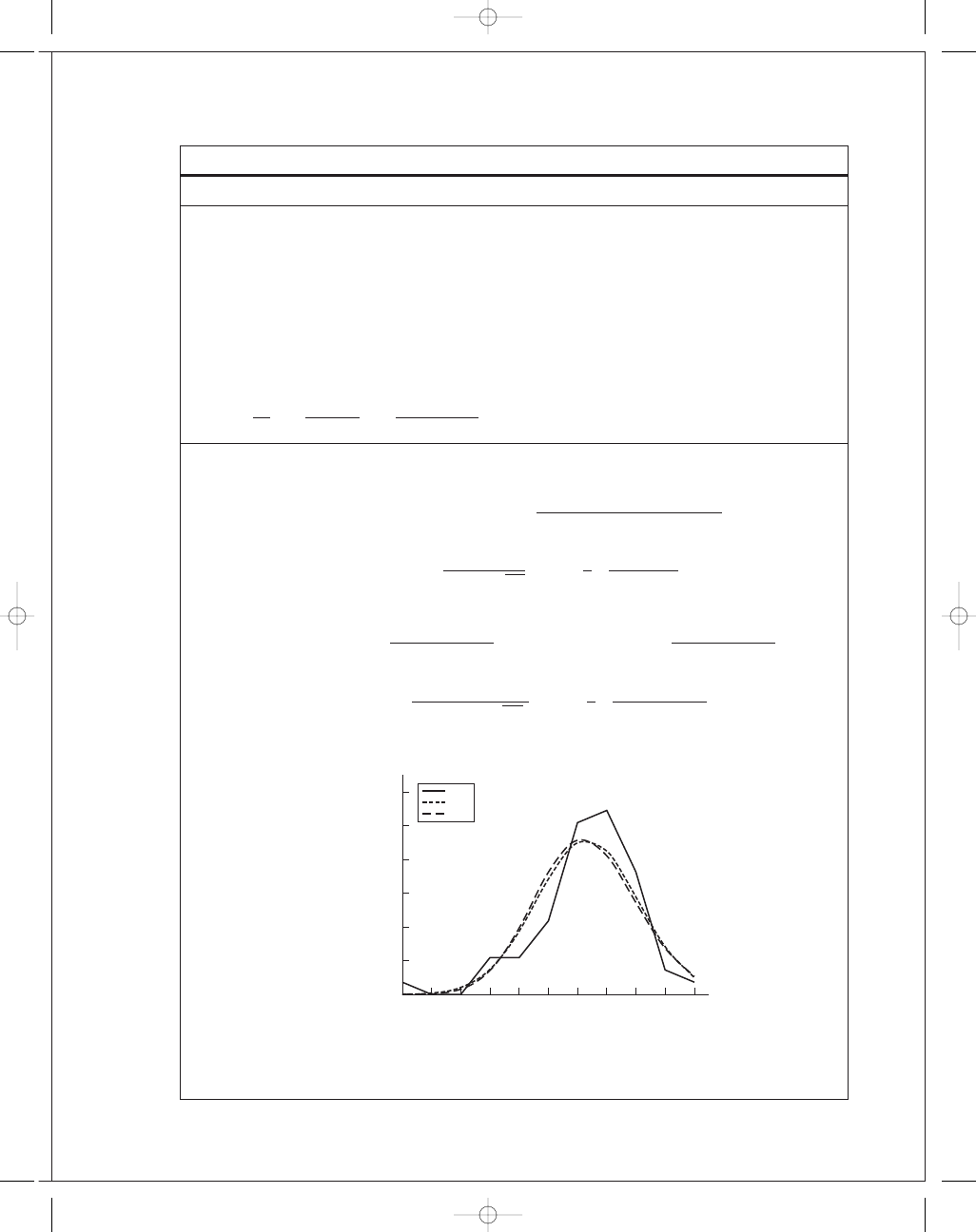
For the Weibull density function, Eq. (2-27),
f
W
(n)
=
2
.66
133
.6 − 36.9
n
− 36.9
133
.6 − 36.9
2
.
66
−
1
exp
−
n
− 36.9
133
.6 − 36.9
2
.
66
For the lognormal distribution, Eqs. (20-18) and (20-19) give,
µ
y
= ln(122.85) − (34.79/122.85)
2
/2 = 4.771
ˆσ
y
=
[1
+ (34.79/122.85)
2
]
= 0.2778
From Eq. (20-17), the lognormal PDF is
f
L N
(n)
=
1
0
.2778 n
√
2
π
exp
−
1
2
ln n
− 4.771
0
.2778
2
We form a table of densities f
W
(n) and f
L N
(n) and plot.
budynas_SM_ch20.qxd 12/06/2006 19:48 Page 22
FIRST PAGES
Chapter 20
23
n (kcycles)
f
W
(n)
f
L N
(n)
40
9.1E-05
1.82E-05
50
0.000 991
0.000 241
60
0.002 498
0.001 233
70
0.004 380
0.003 501
80
0.006 401
0.006 739
90
0.008 301
0.009 913
100
0.009 822
0.012 022
110
0.010 750
0.012 644
120
0.010 965
0.011 947
130
0.010 459
0.010 399
140
0.009 346
0.008 492
150
0.007 827
0.006 597
160
0.006 139
0.004 926
170
0.004 507
0.003 564
180
0.003 092
0.002 515
190
0.001 979
0.001 739
200
0.001 180
0.001 184
210
0.000 654
0.000 795
220
0.000 336
0.000 529
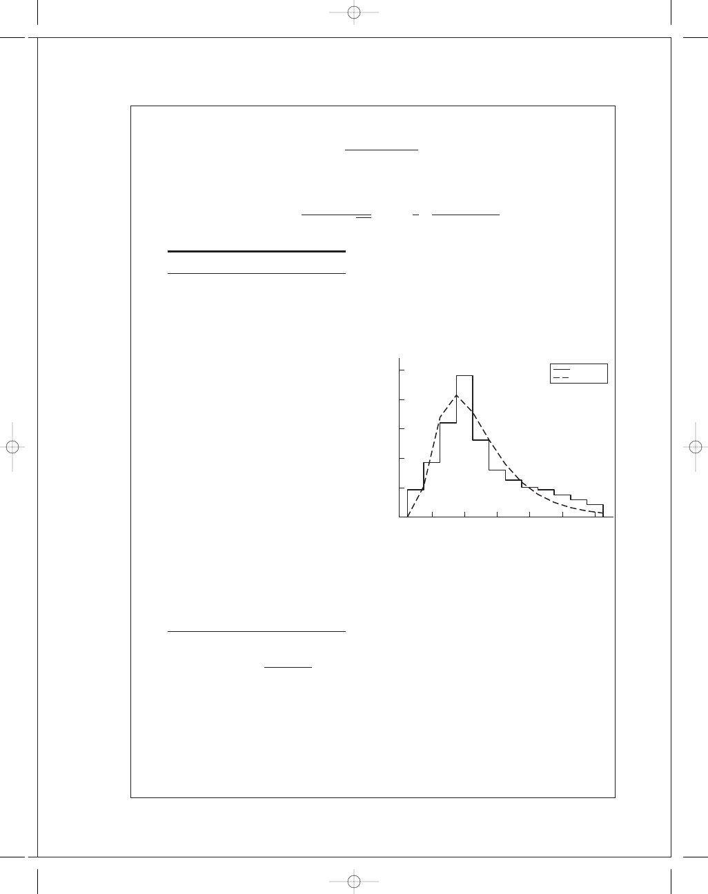
The Weibull L10 life comes from Eq. (20-26) with a reliability of R
= 0.90. Thus,
n
0
.
10
= 36.9 + (133 − 36.9)[ln(1/0.90)]
1
/
2
.
66
= 78.1 kcycles Ans.
The lognormal L10 life comes from the definition of the z variable. That is,
ln n
0
= µ
y
+ ˆσ
y
z
or
n
0
= exp(µ
y
+ ˆσ
y
z)
From Table A-10, for R
= 0.90, z = −1.282. Thus,
n
0
= exp[4.771 + 0.2778(−1.282)] = 82.7 kcycles Ans.
f (n)
n, kcycles
0
0.004
0.002
0.006
0.008
0.010
0.012
0.014
0
100
50
150
200
LN
W
250
budynas_SM_ch20.qxd 12/06/2006 19:48 Page 23
FIRST PAGES
24
Solutions Manual • Instructor’s Solution Manual to Accompany Mechanical Engineering Design
20-33 Form a table
x
g(x)
i
L(10
−
5
)
f
i
f
i
x(10
−
5
)
f
i
x
2
(10
−
10
)
(10
5
)
1
3.05
3
9.15
27.9075
0.0557
2
3.55
7
24.85
88.2175
0.1474
3
4.05
11
44.55
180.4275
0.2514
4
4.55
16
72.80
331.24
0.3168
5
5.05
21
106.05
535.5525
0.3216
6
5.55
13
72.15
400.4325
0.2789
7
6.05
13
78.65
475.8325
0.2151
8
6.55
6
39.30
257.415
0.1517
9
7.05
2
14.10
99.405
0.1000
10
7.55
0
0
0
0.0625
11
8.05
4
32.20
259.21
0.0375
12
8.55
3
25.65
219.3075
0.0218
13
9.05
0
0
0
0.0124
14
9.55
0
0
0
0.0069
15
10.05
1
10.05
101.0025
0.0038
100
529.50
2975.95
¯x = 529.5(10
5
)
/100 = 5.295(10
5
) cycles
Ans.
s
x
=
2975
.95(10
10
)
− [529.5(10
5
)]
2
/100
100
− 1
1
/
2
= 1.319(10
5
) cycles
Ans.
C
x
= s/ ¯x = 1.319/5.295 = 0.249
µ
y
= ln 5.295(10
5
)
− 0.249
2
/2 = 13.149
ˆσ
y
=
!
ln(1
+ 0.249
2
)
= 0.245
g(x)
=
1
x
ˆσ
y
√
2
π
exp
−
1
2
ln x
− µ
y
ˆσ
y
2
g(x)
=
1
.628
x
exp
−
1
2
ln x
− 13.149
0
.245
2
budynas_SM_ch20.qxd 12/06/2006 18:53 Page 24
FIRST PAGES
Chapter 20
25
20-34
x
= S
u
= W[70.3, 84.4, 2.01]
Eq. (20-28)
µ
x
= 70.3 + (84.4 − 70.3)(1 + 1/2.01)
= 70.3 + (84.4 − 70.3)(1.498)
= 70.3 + (84.4 − 70.3)0.886 17
= 82.8 kpsi Ans.
Eq. (20-29)
ˆσ
x
= (84.4 − 70.3)[(1 + 2/2.01) −
2
(1
+ 1/2.01)]
1
/
2
ˆσ
x
= 14.1[0.997 91 − 0.886 17
2
]
1
/
2
= 6.502 kpsi
C
x
=
6
.502
82
.8
= 0.079 Ans.
20-35 Take the Weibull equation for the standard deviation
ˆσ
x
= (θ − x
0
)[
(1 + 2/b) −
2
(1
+ 1/b)]
1
/
2
and the mean equation solved for
¯x − x
0
¯x − x
0
= (θ − x
0
)
(1 + 1/b)
Dividing the first by the second,
ˆσ
x
¯x − x
0
=
[
(1 + 2/b) −
2
(1
+ 1/b)]
1
/
2
(1 + 1/b)
4
.2
49
− 33.8
=
(1 + 2/b)
2
(1
+ 1/b)
− 1 =
√
R
= 0.2763
0
0.1
0.2
0.3
0.4
0.5
10
5
g(x)
x, cycles
Superposed
histogram
and PDF
3.05(10
5
)
10.05(10
5
)
budynas_SM_ch20.qxd 12/06/2006 18:53 Page 25
FIRST PAGES
26
Solutions Manual • Instructor’s Solution Manual to Accompany Mechanical Engineering Design
Make a table and solve for b iteratively
b .
= 4.068 Using MathCad Ans.
θ = x
0
+
¯x − x
0
(1 + 1/b)
= 33.8 +
49
− 33.8
(1 + 1/4.068)
= 49.8 kpsi Ans.
20-36
x
= S
y
= W[34.7, 39, 2.93] kpsi
¯x = 34.7 + (39 − 34.7)(1 + 1/2.93)
= 34.7 + 4.3(1.34)
= 34.7 + 4.3(0.892 22) = 38.5 kpsi
ˆσ
x
= (39 − 34.7)[(1 + 2/2.93) −
2
(1
+ 1/2.93)]
1
/
2
= 4.3[(1.68) −
2
(1
.34)]
1
/
2
= 4.3[0.905 00 − 0.892 22
2
]
1
/
2
= 1.42 kpsi Ans.
C
x
= 1.42/38.5 = 0.037 Ans.
20-37
x (Mrev)
f
f x
f x
2
1
11
11
11
2
22
44
88
3
38
114
342
4
57
228
912
5
31
155
775
6
19
114
684
7
15
105
735
8
12
96
768
9
11
99
891
10
9
90
900
11
7
77
847
12
5
60
720
Sum
78
237
1193
7673
µ
x
= 1193(10
6
)
/237 = 5.034(10
6
) cycles
ˆσ
x
=
7673(10
12
)
− [1193(10
6
)]
2
/237
237
− 1
= 2.658(10
6
) cycles
C
x
= 2.658/5.034 = 0.528
b
1
+ 2/b 1 + 1/b (1 + 2/b) (1 + 1/b)
3
1.67
1.33
0.903 30
0.893 38
0.363
4
1.5
1.25
0.886 23
0.906 40
0.280
4.1
1.49
1.24
0.885 95
0.908 52
0.271
budynas_SM_ch20.qxd 12/06/2006 18:53 Page 26
FIRST PAGES
Chapter 20
27
From Eqs. (20-18) and (20-19),
µ
y
= ln[5.034(10
6
)]
− 0.528
2
/2 = 15.292
ˆσ
y
=
!
ln(1
+ 0.528
2
)
= 0.496
From Eq. (20-17), defining g(x),
g (x)
=
1
x(0
.496)
√
2
π
exp
−
1
2
ln x
− 15.292
0
.496
2
x (Mrev)
f
/(Nw)
g (x)
· (10
6
)
0.5
0.000 00
0.000 11
0.5
0.046 41
0.000 11
1.5
0.046 41
0.052 04
1.5
0.092 83
0.052 04
2.5
0.092 83
0.169 92
2.5
0.160 34
0.169 92
3.5
0.160 34
0.207 54
3.5
0.240 51
0.207 54
4.5
0.240 51
0.178 48
4.5
0.130 80
0.178 48
5.5
0.130 80
0.131 58
5.5
0.080 17
0.131 58
6.5
0.080 17
0.090 11
6.5
0.063 29
0.090 11
7.5
0.063 29
0.059 53
7.5
0.050 63
0.059 53
8.5
0.050 63
0.038 69
8.5
0.046 41
0.038 69
9.5
0.046 41
0.025 01
9.5
0.037 97
0.025 01
10.5
0.037 97
0.016 18
10.5
0.029 54
0.016 18
11.5
0.029 54
0.010 51
11.5
0.021 10
0.010 51
12.5
0.021 10
0.006 87
12.5
0.000 00
0.006 87
z
=
ln x
− µ
y
ˆσ
y
⇒ ln x = µ
y
+ ˆσ
y
z
= 15.292 + 0.496z
L
10
life, where 10% of bearings fail, from Table A-10, z
= −1.282. Thus,
ln x
= 15.292 + 0.496(−1.282) = 14.66
∴ x = 2.32 × 10
6
rev
Ans.
Histogram
PDF
x, Mrev
g
(x
)(10
6
)
0
0.05
0.1
0.15
0.2
0.25
0
2
4
6
8
10
12
budynas_SM_ch20.qxd 12/06/2006 18:53 Page 27
Wyszukiwarka
Podobne podstrony:
budynas SM ch01
budynas SM ch15
budynas SM ch16
budynas SM ch14
budynas SM ch05
budynas SM ch12
budynas SM ch09
budynas SM ch03
budynas SM ch10
budynas SM ch08
budynas SM ch11
budynas SM ch07
budynas SM ch04
budynas SM ch13
budynas SM ch02
budynas SM ch17
budynas SM ch06
więcej podobnych podstron