[20:08 3/11/2009 Bioinformatics-btp563.tex]

Page: 3108

3108–3113

BIOINFORMATICS

ORIGINAL PAPER

Vol. 25 no. 23 2009, pages 3108–3113

doi:10.1093/bioinformatics/btp563

Structural bioinformatics

The interwinding nature of protein–protein interfaces and its
implication for protein complex formation

Kei Yura

1

,2,∗

and Steven Hayward

3

,4,∗

1

Computational Biology, Graduate School of Humanities and Sciences,

2

Center for Informational Biology,

Ochanomizu University, 2-1-1 Otsuka, Bunkyo, Tokyo 112-8610, Japan and

3

School of Computing Sciences and

4

School of Biological Sciences, University of East Anglia, Norwich, NR4 7TJ, UK

Received on April 14, 2009; revised on August 19, 2009; accepted on September 25, 2009

Advance Access publication September 29, 2009

Associate Editor: Thomas Lengauer

ABSTRACT

Motivation: Structural features at protein–protein interfaces can be

studied to understand protein–protein interactions. It was noticed

that in a dataset of 45 multimeric proteins the interface could either

be described as flat against flat or protruding/interwound. In the latter,

residues within one chain were surrounded by those in other chains,

whereas in the former they were not.

Results: A simple method was developed that could distinguish

between these two types with results that matched those made

by a human annotator. Applying this automatic method to a large

dataset of 888 structures, chains at interfaces were categorized as

non-surrounded or surrounded. It was found that the surrounded set

had a significantly lower folding tendency using a sequence based

measure, than the non-surrounded set. This suggests that before

complexation, surrounded chains are relatively unstable and may be

involved in ‘fly-casting’. This is supported by the finding that terminal

regions are overrepresented in the surrounded set.

Availability: http://cib.cf.ocha.ac.jp/DACSIS/

Contact: [e-mail]; [e-mail]

Supplementary information: Supplementary data are available at

Bioinformatics online.

1

INTRODUCTION

Protein–protein interactions, both transient and permanent including
the interactions forming supramolecules, play an essential role in
biological function (Alberts, 1998; Gavin et al., 2006). Prominent
examples are RNA polymerase for transcription, spliceosome for
mRNA maturation and the ribosome for translation. Knowledge
of the components of these complexes and determination of their
atomic structures is essential for understanding mechanism to
function. The components of the complexes can be identified by
mass spectroscopy, yeast two-hybrid systems and other related
methods (Gavin et al., 2006; Krogan et al., 2006) and their structures
can be solved by X-ray crystallography (Dutta and Berman, 2005).

Accumulation of structural data enables the study of protein–protein

interfaces, leading to the prospect of being able to predict complexed
structures given only the structures of the individual components.
Recent studies have demonstrated that the chemical characteristics

∗

To whom correspondence should be addressed.

of interfaces, namely hydrophobicity and complementarity, are
important for prediction (Janin et al., 2008).

Visual inspection of some of protein complex structures reveals

that there is a feature of protein–protein interfaces that has received
little attention, namely that the backbone of one chain protrudes into
other subunits or interwinds with the backbone of other subunits.
The small heat shock protein (sHSP) from wheat, involved in
disaggregation of thermally denatured proteins (van Montfort et al.,
2001), forms a dodecamer. For some monomer crystallographic
structures, 42 residues at the N-terminal are disordered, whereas
the corresponding residues form a coil and a helix in the complexed
structure. In addition the C-terminal end of each subunit protrudes
into the neighbouring subunit (van Montfort et al., 2001). Both
N- and C-termini seem to tether the subunits together, strengthening
subunit interactions. This is supported by a C-terminal truncation
mutant of homologous Hsp104 from Saccharomyces cerevisiae
which has a defect in oligomerization indicating a crucial role of
the C-terminal region in the oligomerization process (Mackay et al.,
2008).

These protruding/interwound regions at interfaces may be a

remnant of docking that involves a process called fly-casting (Levy
et al., 2005; Shoemaker et al., 2000). Fly-casting was proposed
to speed up the recognition of interaction partners while forming
an oligomer or protein–DNA complex. The Go-model simulation
of protein/protein and protein/DNA recognition showed that an
unfolded region in a monomer helps speed up the docking process by
reeling in the partner once the initial contact between the monomers
has been made (Shoemaker et al., 2000). It is plausible that unfolded
N- or C-terminal regions in uncomplexed monomers could fulfill this
role. If so, the N- or C-terminal regions are likely to remain attached
to the other subunit in the complexed structure.

Analysis of the structures of subunit interfaces mentioned above

may pave the way for understanding both static and dynamic
features of protein–protein interactions. There is, however, no
automatic method to identify protruding/interwound regions at
interfaces, and hence no way to assess the significance of these
features in protein–protein interactions. Here, we devised a method
to automatically detect protruding/interwound regions at protein–
protein interfaces and applied it to a set of complexed structures
from the protein structural database. We found that a high proportion
of protein interfaces have regions that are protruding/interwound.
These regions are often located at the termini of individual

© The Author(s) 2009. Published by Oxford University Press.
This is an Open Access article distributed under the terms of the Creative Commons Attribution Non-Commercial License (http://creativecommons.org/licenses/
by-nc/2.5/uk/) which permits unrestricted non-commercial use, distribution, and reproduction in any medium, provided the original work is properly cited.

at Uniwertytet Gdanski on June 11, 2014

http://bioinformatics.oxfordjournals.org/

Downloaded from

[20:08 3/11/2009 Bioinformatics-btp563.tex]

Page: 3109

3108–3113

The interwinding nature of protein–protein interfaces

subunits, although sometimes they are located at non-terminal
loops. Analysing their sequences showed that these regions have a
greater propensity to be unfolded than non-interwound/protruding
regions. We further speculate on the role of these regions in protein
complexation.

2

DATA AND METHODS

2.1

Collection of protein oligomer 3D structures and
subunit interfaces

Protein oligomer 3D structures from the March 2007 release of the Protein
Databank (PDB) (Berman et al., 2007) were selected by the following
procedure. First, an entry from the PDB with two or more polypeptides
was selected. An entry with DNA/RNA molecules was discarded. To make
sure that the polypeptides form a complexed structure, all the distances of
atoms from each polypeptide were calculated and when 40 or more pairs of
atoms were located within 4.5 Å, then the two polypeptides were considered
to be in complexed state. An oligomer is defined as a set of polypeptides with
each polypeptide having, at least, another polypeptide that forms a complex
with it. Second, the most similar amino acid sequence from UniProt (The
UniProt Consortium, 2008) against one of the sequences in the oligomer was
selected using BLAST (Altschul et al., 1997) with default parameters. Each
UniProt entry contains a description of the number of biologically relevant
subunits in the comment line. The number of chains in the oligomer and
the number of subunits described in UniProt were compared, and when the
number was different, the oligomer entry was discarded. Taking advantage
of the systematic nomenclature of UniProt entry ID, the oligomers with
homologous amino acid sequences were grouped. The nomenclature of
UniProt entry ID is a shortened form of the protein family name followed by
an underscore and a shortened species name. Therefore, oligomers with the
same protein family name could be grouped using the UniProt entry ID. Each
group was then represented by a single oligomer: the one with the highest
resolution and fewest disordered atoms. Entries with missing atoms in the
subunit interfaces were discarded.

2.2

Measuring the degree of surroundedness of
residues at the interfaces; surroundedness factor

The extent to which residues within one chain were protruding/interwound
with other chains was quantified in the following manner. We extended
and modified the method named CX (Pintar et al., 2002), which was
developed to identify atoms protruding into the solvent, in order to identify
protruding/interwound segments at subunit interfaces. The i-th residue along
the sequence at the interface was represented by its C

α atom, and the number

of non-hydrogen atoms belonging to the same polypeptide (N

s

) and the

number of non-hydrogen atoms belonging to a different polypeptide (N

d

),

both located within a fixed distance R from the C

α atom, were counted. We

defined the surroundedness factor (SF) of residue i at the interface as

SF

R

,i

=

1

2L

+1

L

k

=−L

N

d

i

+k

N

s

i

+k

,

where L governs the amount of smoothing along the amino acid sequence
around the i-th residue. L relates to a window length as W

= 2L + 1. If the

interfaces of both subunits are flat, then SF would be close to 1.0, and if
the interface is protruding into, or interwound with, chains of other subunits,
then SF would be much greater than 1.0. A value of 12 Å was used for R
close to the 10 Å default value used for CX (Pintar et al., 2002) and a value of
five residues was used for W . The best threshold value of SF to distinguish
between flat and protruding/interwound segments was a parameter to be
determined.

2.3

Measuring the folding tendency of a fragment

The folding of the polypeptide at the subunit interface may have been induced
by subunit interactions. We predicted whether part of the sequence at the

interface was intrinsically unfolded using FoldIndex (Prilusky et al., 2005;
Uversky et al., 2000). FoldIndex I

KD

F

is a simple measure to predict whether

the amino acid sequence is likely to be folded or intrinsically unfolded based
on the mean net charge and the mean hydrophobicity of the sequence:

I

KD

F

=2.785H−|R|−1.151,

where

H is the sum of all residue hydrophobicities divided by the total

number of residues, and

|R| is the absolute value of the difference between

the number of positively charged residues and the number of negatively
charged residues at pH 7 divided by the total number of residues. The
hydrophobicity was measured using the Kyte and Doolittle (1982) scale,
with parameters between 0.0 and 1.0. When I

KD

F

is positive, the sequence is

likely to fold, and when it is negative, the sequence is likely to be intrinsically
unfolded (Prilusky et al., 2005).

3

RESULTS

3.1

The number of oligomer 3D structures

We gathered 888 PDB entries with multi-subunit structures. In
these entries, there were 976 unique subunits based on our standard
described in Section 2. Of the 888 entries, 580 entries were dimers
(2), 72 were trimers (3), 162 were tetramers (4), nine were pentamers
(5), 43 were hexamers (6), two were heptamers (7), eight were
octamers (8), two were decamers (10), one was undecamer (11),
six were dodecamers (12), one tetradecamer (14), one hexadecamer
(16) and one tetracosamer (24). Of the 888 entries, 815 entries were
homo-oligomers and 73 entries were hetero-oligomers. We used
one chain from each homo-oligomers and 161 non-homologous
chains from hetero-oligomers, hence 976 chains were analysed.
Further details on the 888 structures and 976 chains can be found at
http://cib.cf.ocha.ac.jp/DACSIS/.

3.2

Determination of threshold value for SF

SF was newly introduced to automatically measure the degree
of protruding/interwound segments in protein–protein interfaces.
In order to determine a good threshold for SF to distinguish
between a segment with a flat-against-flat interface (not surrounded)
and one with a protruding/interwound interface (surrounded), 45
examples were selected at random from the 888 structures. Of
these 45 complexes, segments of the polypeptide at the subunit
interfaces were categorized by visual inspection using molecular
graphics, as being surrounded by the other subunit. Excluding
equivalent residues in symmetry related subunits, 17 segments
comprising 254 residues from 13 complexes were put in the
‘surrounded’ set. In the remaining 32 complexes, interface residues
were identified as those that had SF

> 0, with R = 6 Å and W = 1.

Removing symmetrically equivalent residues gave 1395 residues in
189 segments in the ‘non-surrounded’ set. SF, now with R

= 12 Å

and W

= 5 residues, was calculated for each of these residues in

each of these sets. For the non-surrounded set the mean SF value
was 0.421 [standard deviation (SD) 0.238] and for the surrounded
set the mean SF value was 1.085 (SD 0.68). A two-sample t-test
gave a t-value of 15.4 [probability(t

>15.4) 10

−6

] which shows

a highly significant difference between the two sets. The difference
between the two sets is also supported by a Mann–Whitney U-test
[U = 62 812, z = 16.38, probability(z)

10

−6

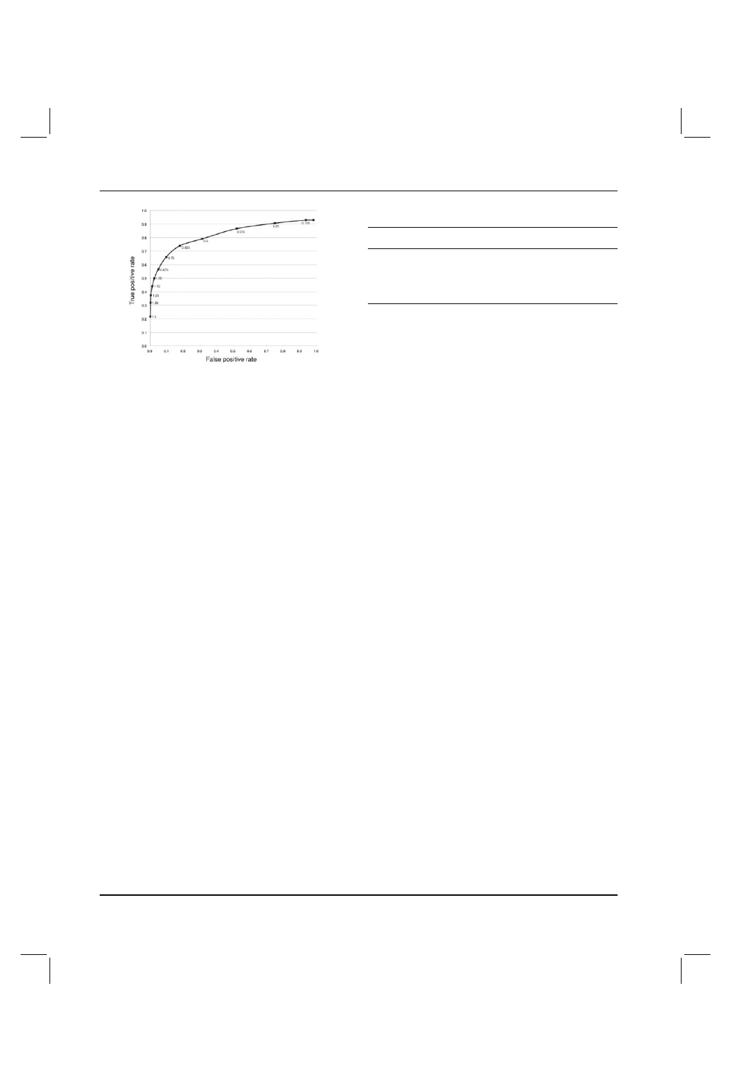
]. Figure 1 shows the

receiver operating characteristic (ROC) curve where the true positive
rate (proportion of surrounded set greater than threshold SF value) is
plotted against the false positive rate (proportion of non-surrounded

3109

at Uniwertytet Gdanski on June 11, 2014

http://bioinformatics.oxfordjournals.org/

Downloaded from

[20:08 3/11/2009 Bioinformatics-btp563.tex]

Page: 3110

3108–3113

K.Yura and S.Hayward

Fig. 1. ROC curve for the determination of the SF threshold. Below 1.25,
the false positive rate is practically zero. The horizontal axis is the proportion
of the non-surrounded set greater than the threshold SF value (false positive
rate) and the vertical axis is proportion of surrounded set greater than the
threshold SF value (true positive rate). Each threshold value is shown on
the plot.

set greater than threshold SF value) and each point represents a
threshold value for SF. Based on this curve and with a view that the
number of false positives should be as practically low as possible,
a threshold value of 1.25 for SF was selected. Even though only
about one-third of the residues in the surrounded set were correctly
identified, when considering whole segments, this threshold value
gave a good result: for the 17 segments in the surrounded set, 14
had at least one residue with a SF value

≥1.25, whereas for the

non-surrounded set, only two segments out of 189 had at least one
residue with a SF value

≥1.25. Thus a threshold value of 1.25 for

SF is able to automatically distinguish between surrounded and non-
surrounded segments in a way that conforms to a human annotator
using molecular graphics. This allows us to use SF to distinguish
surrounded and non-surrounded regions in the much larger set of
protein complexes.

3.3

Application of SF to the whole data

The SF calculation was applied to 976 chains in 888 oligomer
entries. The 976 chains comprise 257 831 residues of which 137 865
residues (53.4%) have non-zero SF values. These residues are
defined as interface residues. All the data is available at http://cib
.cf.ocha.ac.jp/DACSIS/. The SF data is presented in raw format as
well as graphically. In addition, the 3D structures of proteins with
the high SF segments can be viewed using the molecular graphics
software Jmol (http://www.jmol.org/).

3.4

High SF segments occur with high significance in
terminal regions

Out of the whole data, segments were selected that contained the
longest run of consecutive residues with SF

≥1.25. The two residues

on the N-terminal flank and the two residues on the C-terminal
flank were also included. We added two residues on both termini
of the segment, because SF of the segment is calculated with
W

= 5. We identified 562 segments of high SF (≥1.25) in 362 chains

out of the whole set comprising 976 chains (Table 1). These are

Table 1. Distribution of high SF in the terminal regions

Location

High SF segment

a

High SF residue

Count of residue

N-terminal

113 (20.1%)

374 (13.9%)

7808 (3.1%)

Middle

337 (60.0%)

1906 (71.0%)

238 311 (93.8%)

C-terminal

112 (19.9%)

406 (15.1%)

7808 (3.1%)

Total

562 (100%)

2686 (100%)

253 927 (100%)

a

Terminal region is defined as 10-residue range from the terminal residue. When one

of the residues in high SF segment is located within the region, it is counted.

the surrounded set for the whole dataset. Of the 562 segments,
113 segments are located within a 10-residue range of the N-terminal
and 112 segments within 10-residue range of the C-terminal. The
remaining 337 segments are located in the internal region of the
chain. To check whether this distribution is not random, our null
hypothesis would be that the non-zero SF residues are randomly
located on the protein chains. We performed the following test in
the count of residues, not in the count of segments for simplicity.
Since a non-zero SF residue is only found at an interface, high SF
segments should be evenly distributed in the interfaces according to
the null hypothesis. The 976 chains contain 137 865 residues with
non-zero SF value. The number of residues in terminal regions
is 15 616 ( = 8

×976 ×2) (Table 1). Note that since W = 5, two

residues on both termini cannot be assigned a SF value. Thus
the expected number of residues with high SF values in terminal
regions is

∼165.2 [=(2686/253 927)×15 616]. A χ

2

-test of the

observed distribution of the residues in terminal regions with high
SF values [780 (=374 (N-terminus) + 406 (C-terminus)] showed that
the distribution is extremely skewed and not random [

χ

2

= 2288

probability(

χ

2

>2288) 10

−6

]. It should be noted, however, that

337 segments, a non-negligible number (Table 1), with high SF
values are located in the internal regions, mostly as loops.

3.5

Example of high SF segment at the terminal region
and in the loop

SF was calculated on protein kinase domain of a trp Ca-channel,
ChaK (PDB ID: 1IA9) as one of the examples (not used for
the adjustment of the threshold). Applying the threshold value
for SF (

≥1.25) to automatically detect the protruding/interwound

segments in the interface worked well as shown in Figures 2a
and b. Visual inspection shows that only the N-terminal residues
of subunit A are surrounded by subunit B (Fig. 2a), corresponding
to the automatic method where only the N-terminal residues 3 and
12–24 have SF values

≥1.25 (Fig. 2b). At a glance, exclusion of

the N-terminal half of the helix seems unreasonable. However, the
whole helix is not inserted into chain B and the N-terminal part of
the helix is located far from chain B. The N-terminal residues before
the helix are very close to chain B. Hence the SF calculation with
the threshold value of 1.25 gives a reasonable result in this case.

SF was also calculated on C-type lectin CRD domain bound to

coagulation factor IX-binding protein (PDB ID: 1BJ3) as an example
with the high SF region in a loop (Fig. 2c and d). Residues 82–86
of C-type lectin CRD domain are located on the tip of a long loop
and extensively interact with the other subunit. Other regions of the
loop are relatively exposed to the solvent.

3110

at Uniwertytet Gdanski on June 11, 2014

http://bioinformatics.oxfordjournals.org/

Downloaded from

[20:08 3/11/2009 Bioinformatics-btp563.tex]

Page: 3111

3108–3113

The interwinding nature of protein–protein interfaces

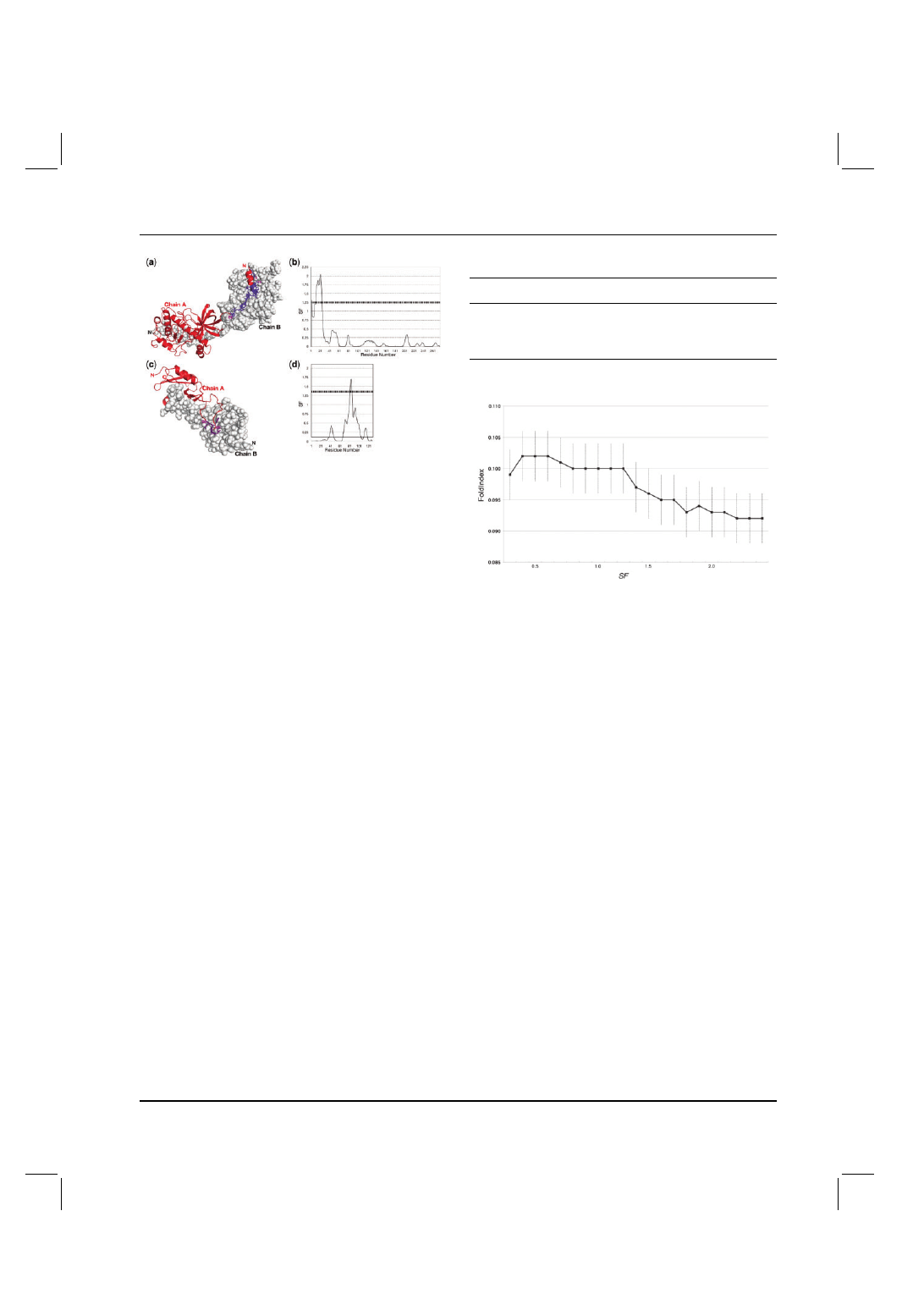
Fig. 2. Result of SF calculation on the kinase domain of Trp Ca-channel,
ChaK (PDB ID: 1IA9) homodimer (a and b) and C-type lectin CRD domain
bound to coagulation factor IX-binding protein (PDB ID: 1BJ3) (c and d).
SF was calculated on one of the subunits only (chain A). (a) Residues
with SF

≥ 1.25 on ChaK protein are with side chains and coloured in deep

purple. Other residues are coloured in red. (b) SF values of ChaK chain A.
(c) Residue with SF

≥1.25 on C-type lectin CRD domain. (d) SF values on

C-type lectin CRD domain.

3.6

FoldIndex indicates that surrounded segments are
more likely to be disordered than non-surrounded

A surrounded set segment was defined at the beginning of

Section 3.4. A non-surrounded set segment was defined as one that
contained the longest run of consecutive residues with 0

< SF < 1.25

plus the two residues on the N-terminal flank and the two residues
on the C-terminal flank (thus the minimum fragment length is five
residues as W = 5). There are 562 segments in the surrounded set and
5557 segments in the non-surrounded set. Protruding/interwound
segments in the surrounded group have substantial interactions
with other subunits, hence before complexation, the segment does
not have these interactions and evidently does not assume the
same structure as the one observed in the complexed structure.
Therefore, a likely scenario is that the segments are unfolded
before complexation. If so, a measure of intrinsic liability to fold
should indicate a difference between these two groups. FoldIndex
is a simple sequence-based measure that is supposed to measure a
segment’s intrinsic liability to fold or remain unfolded (Prilusky
et al., 2005; Uversky et al., 2000). If its value is positive it
indicates a polypeptide that has a propensity to fold, whereas if
its value is negative it indicates a polypeptide with a propensity
to remain unfolded. We applied FoldIndex to the two groups and
found that its average value for the non-surrounded group was
0.1193 (SD = 0 .23 from 5557 segments), whereas for the surrounded
group it had an average value of 0.0286 (SD = 0.33 from 562
segments) (Table 2). This result was tested using a two-sample
t-test and found to be highly significant [t = 6.4, probability(t

>6.4)

10

−6

]. The significant difference between the two groups is also

supported by a Mann–Whitney U-test [U = 1.69

×10

6

, z = 10.37,

probability(z)

10

−6

]. The average length of the segments in the

surrounded group is 8.7 residues, whereas the average length of the
segments in the non-surrounded group is 28.0 residues (The length
distribution is shown in Supplementary Materials). This calculation
weights equally, short and long segments which could introduce

Table 2. Correlation of SF and FoldIndex

SF

Count

FoldIndex (SD)

a

<1.25

5557

0.119 (

±0.23)

≥ 1.25

562

0.0286 (

±0.33)

Total

6119

a

A two-sample t-test result in t = 6.4 (P

10

−6

)

.

Fig. 3. Cumulative distribution of average FoldIndex values against SF.
Each point indicates an average value (with standard error) of FoldIndex of
the segments with SF values less than the specified value.

a bias. In order to overcome this, a sliding window with five-
residue length was applied to each segment thus creating a set
of sequences each of equal length. FoldIndex was then applied to
each of the pentapeptide sequences in the two groups. The average
value for the surrounded group was 0.0122 (SD = 0.432 from 2657
pentapeptides), whereas for the non-surrounded group it had an
average value of 0.0399 (SD = 0.4694 from 133 416 pentapeptides).

Again this result was tested using a two-sample t-test and also

found to be highly significant [t = 3.3, probability(t

>3.3) ≈0.05%].

The difference between the two groups is also supported again by
a Mann–Whitney U-test [U = 1.84

×10

8

, z

>10

2

, probability(z)

10

−6

]. The statistical tests above suggest that there is a negative

correlation between SF and FoldIndex. This is verified in the
cumulative graph of Figure 3. In this cumulative graph, the point at
SF = 1.0, for instance, means the average value of all the FoldIndex
values of segments with SF

≤1.0. As the upper limit on SF gets

higher, so the average of the FoldIndex value gets lower. The
cumulative graph shows a sharp drop between SF = 1.2 and 1.3
which corresponds to the threshold value for automatically detecting
surrounded regions. As a lower FoldIndex value indicates a greater
tendency to be disordered, this negative correlation supports our
hypothesis that the surrounded set is less ordered in the uncomplexed
state than the non-surrounded set.

3.7

Application of SF to a different data set

The data set we built may contain non-biological interfaces, even
though we cross-validated with UniProt (Section 2). We cannot
rule out the possibility that the biological interface is located
between unit cells. Another possibility is that our dataset does
not represent the true distribution of the interfaces, because we

3111

at Uniwertytet Gdanski on June 11, 2014

http://bioinformatics.oxfordjournals.org/

Downloaded from

[20:08 3/11/2009 Bioinformatics-btp563.tex]

Page: 3112

3108–3113

K.Yura and S.Hayward

did not take symmetric units into account. We, therefore, applied
our SF and FoldIndex analysis to the set of protein interfaces
presented by Keskin et al. (2004) which took crystal symmetry into
account (3799 entries). We found the same significant difference
in the FoldIndex of the surrounded and non-surrounded sets for
this dataset [probability(t

> 9.2) 10

−6

, U = 2.73

×10

7

, z

>10

2

,

probability(z)

10

−6

] and negative correlation between SF and

FoldIndex almost exactly reproduces what is seen in Figure 3.
Hence, the results presented here are likely to be free from
dataset bias.

4

DISCUSSION

We have used simple and easily reproducible methods to
analyse properties at subunit–subunit interfaces with the aim of
understanding processes involved in the formation of protein
complexes. We showed that segments with high SF values have
a significantly lower FoldIndex than those with low SF values.
This suggests that segments that protrude into, or interwind with,
a neighbouring subunit may have a lower propensity to fold. A
possible explanation is that segments with high SF values are
disordered in non-complexed state, but adopt a definite 3D structure
in the complexed state. Truly disordered proteins or disordered
protein segments should have negative FoldIndex values. However,
the high SF regions have an average positive FoldIndex values
close to zero suggesting that these regions may have intermediate
propensities for being ordered and disordered. This may relate to
so-called ‘dual personality’ fragments in proteins (Zhang et al.,
2007). Dual personality fragments are those that have been found
to have a well-defined structure in one X-ray experiment, but
found to be unresolvable in another. An example given in the
paper (Zhang et al., 2007) concerns cyclin dependent kinase, which
has unresolved fragments in one structure, but these fragments
have definite structure in another when it is phosphorylated and
bound to another protein (cyclin). The maximum SF values of the
two fragments, namely Ile35-Val44 and Leu148-Glu162 (PDB ID:
1QMZ chain A), are 1.14 and 0.97, respectively, which are high,
although below the cutoff of 1.25 used here. Their FoldIndex values
are

−0.09 and −1.15, respectively, indicating a small tendency to be

disordered in the former and a strong tendency to be disordered in
the latter. Although phosphorylation may play a role in this example,
it is clear that the cyclin protein also plays a role, as the fragments’
SF values are relatively high. Thus, this example of dual personality
fragments is surely related to the hypothesis that partially unfolded
regions are involved in protein–protein interactions and adopt a
protruding structure upon complexation with a partner protein.

These protruding/interwound segments at interfaces may be a

remnant of the fly-casting process (Levy, et al., 2005; Shoemaker
et al., 2000), whereby an unfolded region in a monomer makes
the initial contact with the partner biomolecule and reels itself in
as the unfolded region folds. A possible scenario would involve
an unfolded region, which is part of a largely folded monomer.
This would increase probability of capture by increasing the search
radius. The folding of the unstructured region would then occur as a
final stage in the docking process, leaving the initially unstructured
region as a remnant, now structured and having substantial contacts
with the partner. It is easier to imagine that this occurs in a partially
folded protein by fly casting an unfolded terminal region rather than

Fig. 4. Example of SF in domain swapping found in the homo-dimer of
bovine seminal ribonuclease (PDB ID: 11BA). One of the monomers is in
green and the other in yellow. The high SF region is in red. N-terminal

α

helices are swapped.

an unfolded loop and this would explain the high proportion of
N- and C-termini in the surrounded dataset.

Segments in the surrounded set were found in 362 (see

Section 3.4) out of 976 chains (see Section 3.3) suggesting that
in more than one third (= 362/976) of known protein complexes,
disordered segments of a protein play a substantial role in complex
structure formation. Of those 362 chains, we found 562 (see Section
3.4) segments in the surrounded set indicating that in some cases
multiple segments are involved in the fly-casting process.

A similar process would also be expected to occur in domain

swapping where part of a monomer structure becomes unfolded
and interwinds with another identical monomer to form a dimer
in an oligomerization process (Rousseau et al., 2003). The
interfaces, especially the subunit-crossing linkers, are unlikely to
be complementary and so in order to make a stable multimer, there
needs to be some interwinding as can be seen in the examples given
in Figure 2 of the paper by Rousseau et al. We have taken as an
example the case of bovine seminal ribonuclease from Figure 2 of
the paper. The protein is the first RNase found to swap domains
and we found high SF regions in a C-terminal part of the swapped
N-terminal

α helix (Fig. 4). The N-terminal region of the α helix

protrudes into solvent and the high SF region which precedes it is
surrounded by the other subunit (average SF = 1.42). Based on our
findings we would expect the high SF region (with the sequence:
FERQHMDSGN) to have a low FoldIndex which indeed it has
(

−0.42). We speculate therefore that the pre-folded α helix on

the N-terminus is fly-casted by this unfolded segment to the other
subunit, which it reels in until the unfolded segment is attached
appropriately to the main part of the other subunit resulting in an
exchange of

α helices.

ACKNOWLEDGEMENTS

The authors thank Dr Nobuhiro Go for his encouragement to
carry out this study, Dr Gavin Cawley for helpful discussions and
Ms Tomo Yuasa for assisting in building the database and website.

Funding: ‘Computational Study on Conformational Changes in
Proteins of Supra-Molecules’ in Strategic International Cooperative
Program of Japan Science and Technology Agency (JST). Targeted
Proteins Research Program (TPRP) from Ministry of Education,
Culture, Sports, Science and Technology (MEXT), Japan.

Conflict of Interest: none declared.

3112

at Uniwertytet Gdanski on June 11, 2014

http://bioinformatics.oxfordjournals.org/

Downloaded from

[20:08 3/11/2009 Bioinformatics-btp563.tex]

Page: 3113

3108–3113

The interwinding nature of protein–protein interfaces

REFERENCES

Alberts,B. (1998) The cell as a collection of protein machines: preparing the next

generation of molecular biologists. Cell, 92, 291–294.

Altschul,S.F. et al. (1997). Gapped BLAST and PSI-BLAST: a new generation of protein

database search programs. Nucleic Acids Res., 25, 3389–3402.

Berman,H. et al. (2007). The worldwide Protein Data Bank (wwPDB): ensuring a single,

uniform archive of PDB data. Nucleic Acids Res., 35, D301–D303.

Dutta,S. and Berman,H.M. (2005) Large macromolecule complexes in the Protein Data

Bank: a status report. Structure, 13, 381–388.

Gavin,A.C. et al. (2006) Proteome survey reveals modularity of the yeast cell machinery.

Nature, 440, 631–636.

Janin,J. et al. (2008) Protein-protein interaction and quaternary structure. Quart. Rev.

Biophys., 41, 133–180.

Keskin,O. et al. (2004) A new, structurally nonredundant, diverse data set of protein-

protein interfaces and its implications. Protein Sci., 13, 1043–1055.

Krogan,N.J. et al. (2006) Global landscape of protein complexes in the yeast

Saccharomyces cerevisiae. Nature, 440, 637–643.

Kyte,J. and Doolittle,R.F. (1982). A simple method for displaying the hydropathic

character of a protein. J. Mol. Biol., 157, 105–132.

Levy,Y. et al. (2005) A survey of flexible protein binding mechanisms and their transition

states using native topology based energy landscpaes. J. Mol. Biol., 346, 1121–1145.

Mackay,R.G. et al. (2008) The C-terminal extension of Saccharomyces cerevisiae

Hsp104 plays a role in oligomer assembly. Biochemistry, 47, 1918–1927.

van Montfort,R.L.M. et al. (2001). Crystal structure and assembly of eukaryotic small

heat shock protein. Nature Struct. Biol., 8, 1025–1030.

Pintar,A. et al. (2002). CX, an algorithm that identifies protruding atoms in proteins.

Bioinformatics, 18, 980–984.

Prilusky,J. et al. (2005). FoldIndex: a simple tool to predict whether a given protein

sequence is intrinsically unfolded. Bioinformatics, 21, 3435–3438.

Rousseau,F. et al. (2003) The unfolding story of three-dimensional domain swapping.

Structure, 11, 243–251.

Shoemaker,B.A. et al. (2000) Speeding molecular recognition by using the folding

funnel: The fly-casting mechanism. Proc. Natl Acad. Sci. USA, 97, 8868–8873.

The UniProt Consortium (2008). The Universal Protein Resource (UniProt). Nucl. Acids

Res., 36, D190–D195.

Uversky,V.N. et al. (2000). Why are "natively unfolded" proteins unstructured under

physiologic conditions? PROTEINS: Struct. Funct. Genet., 41, 415–427.

Zhang,Y. et al. (2007) Between order and disorder in protein structures: analysis of

‘dual personality’ fragments in proteins. Structure, 15, 1141–1147.

3113

at Uniwertytet Gdanski on June 11, 2014

http://bioinformatics.oxfordjournals.org/

Downloaded from