September 7, 2000

Fourier Transforms

1

Finite Fourier Transform

Any discussion of finite Fourier transforms and MATLAB immediately encoun-
ters a notational issue – we have to be careful about whether the subscripts start
at zero or one. The usual notation for finite Fourier transforms uses subscripts
j and k that run from 0 to n − 1. MATLAB uses notation derived from matrix
theory where the subscripts run from 1 to n, so we will use y

j+1

for mathemat-

ical quantities that will also occur in MATLAB code. We will reserve i for the
complex unit,

√

−1.

The finite, or discrete, Fourier transform of a complex vector y with n ele-

ments y

j+1

, j = 0, . . . n − 1 is another complex vector Y with n elements

Y

k+1

=

n−1

X

j=0

y

j+1

e

−2ijkπ/n

, k = 0, . . . , n − 1

The exponentials are all complex n-th roots of unity, i.e. they are all powers of

ω = e

−2πi/n

= cos δ

− i sin δ

where δ = 2π/n. The transform can also be expressed with matrix-vector
notation

Y = F y

where the finite Fourier transform matrix F has elements

f

k+1,j+1

= ω

jk

It turns out that F is nearly its own inverse. More precisely, the complex

conjugate transpose of F satisfies

F

H

F = nI

so

F

−1

=

1

n

F

H

This allows us to invert the Fourier transform.

y =

1

n

F

H

Y

Hence

y

j+1

=

1

n

n−1

X

k=0

Y

k+1

e

2ijkπ/n

, j = 0, . . . , n − 1

1

We should point out that this is not the only notation for finite Fourier

transform in common use. The minus sign in the complex exponentials in the
first equation, and in the definiton of ω, sometimes occurs in the inverse trans-
pose instead. And the 1/n scaling factor in the inverse transform is sometimes
replaced by 1/

√

n scaling factors in both transforms.

In MATLAB, the Fourier matrix F could be generated for any given n by

omega = exp(-2*pi*i/n);
j = 0:n-1;
k = j’
F = omega.^(k*j)

The quantity k*j is an outer product, an n-by-n matrix whose elements are the
products of the elements of two vectors. However, the built-in function fft
takes the finite Fourier transform of each column of a matrix argument, so an
easier, and quicker, way to generate F is

F = fft(eye(n))

The function fft uses a fast algorithm to compute the finite Fourier trans-

form. The first ”f” stands for both ”fast” and ”finite”. A more accurate name
might be ffft, but nobody wants to use that. We will discuss the fast aspect
of the algorithm in a later section.

2

fftshow

The GUI fftshow allows you to investigate properties of the finite Fourier trans-
form. If y is a vector containing a few dozen elements.

fftshow(y)

produces four plots

real(y)

imag(y)

real(fft(y))

imag(fft(y))

You can use the mouse to move any of the points in any of the plots and the
points in the other plots will respond.

Please run fftshow and try the following examples. Each illustrates some

property of the Fourier transform. When you start with no arguments

fftshow

all four plots are initialized to zeros(1,32). Click your mouse in the upper left
hand corner of the upper left hand plot. You will be taking the fft of the first
unit vector, with one in the first component and zeros elsewhere. This should
produce

2

real(y)

imag(y)

real(fft(y))

imag(fft(y))

The real part of the result is constant and the imaginary part is zero. You

can also see this from the definition

Y

k+1

=

n−1

X

j=0

y

j+1

e

−2ijkπ/n

, k = 0, . . . , n − 1

when y

1

= 1 and y

2

= · · · = y

n

= 0. The result is

Y

k+1

= 1 · e

0

+ 0 +

· · · + 0 = 1, for all k

Click on y

1

again, hold the mouse down, and move the mouse vertically. The

amplitude of the constant result varies accordingly.

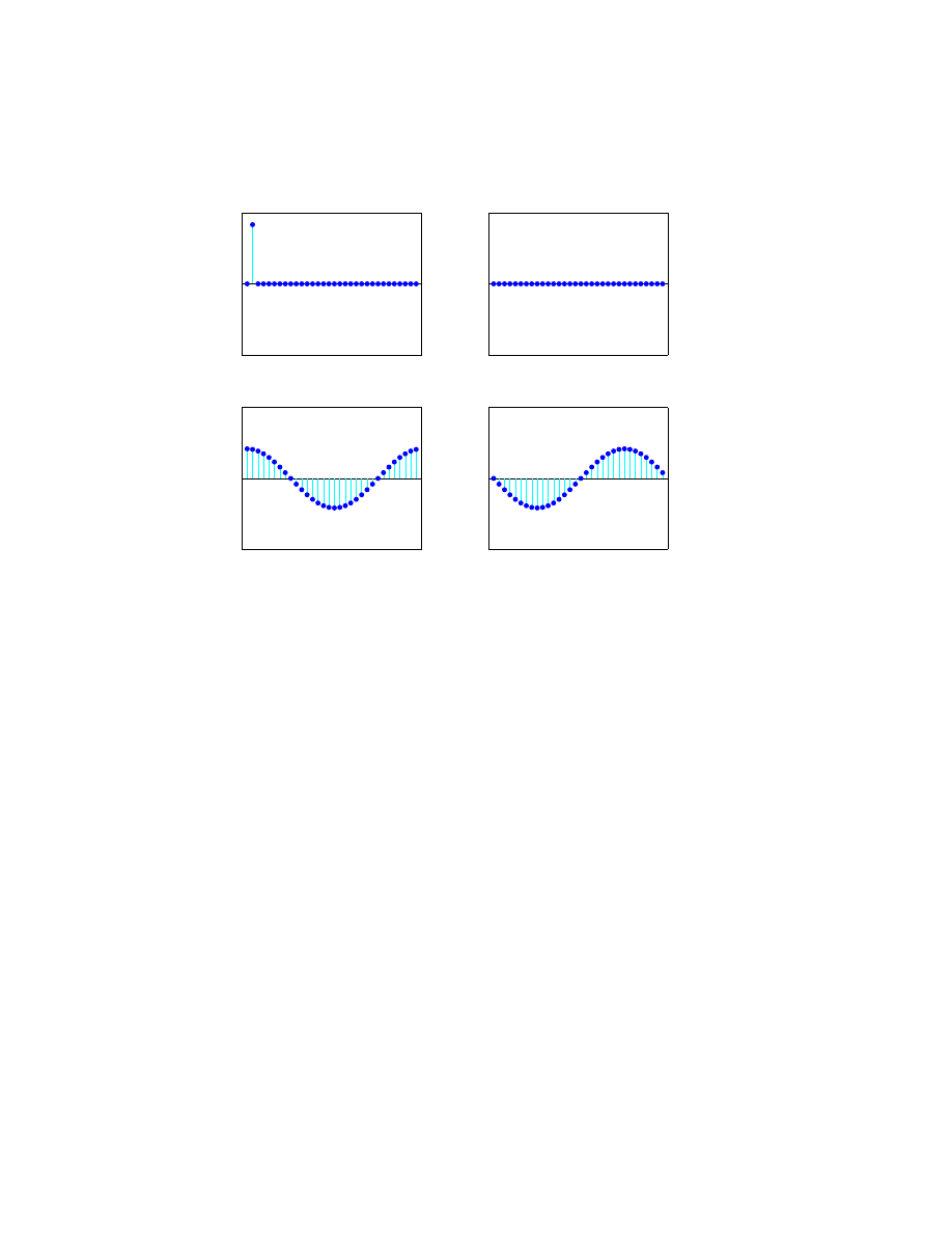
Next, try the second unit vector. Use the mouse to set y

1

= 0 and y

2

= 1.

This should produce

3

real(y)

imag(y)

real(fft(y))

imag(fft(y))

You are seeing the graph of

Y

k+1

= 0 + 1 · e

−2ikπ/n

+ 0 + · · · + 0

Using δ = 2π/n,

real(Y

k+1

) = cos kδ, imag(Y

k+1

) = − sin kδ

for k = 0,

· · · , n − 1. We have sampled two trig functions at n equally spaced

points in the interval 0

≤ x < 2π. The first sample point is x = 0 and the last

sample point is x = 2π − δ.

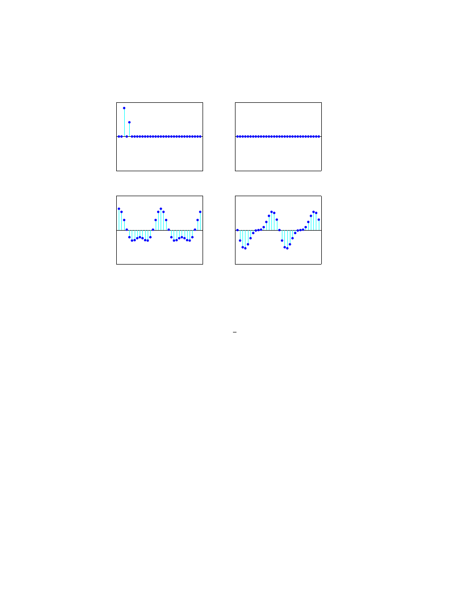
Now set y

3

= 1 and vary y

5

with the mouse. One snapshot is

4

real(y)

imag(y)

real(fft(y))

imag(fft(y))

We have graphs of

cos 2kδ + η cos 4kδ, and − sin 2kδ − η sin 4kδ

for various values of η = y

5

The point just to the right of the center of these graphs is particularly

important. We will call it the Nyquist point. With the points numbered from 1
to n for even n, it’s the point with index

n

2

+ 1. When n = 32, it’s point number

17, just under the left parenthesis in the title.

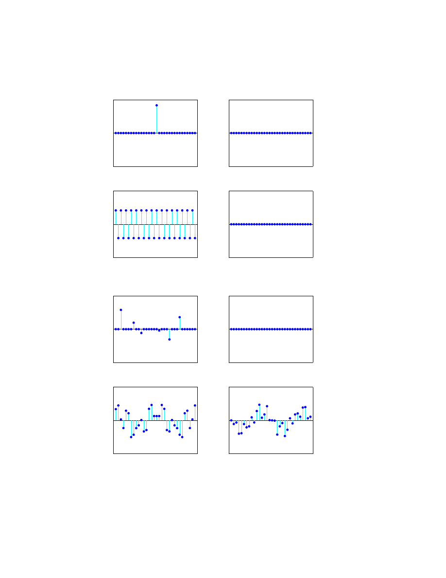
Here is fftshow with a unit vector at the Nyquist point.

5

real(y)

imag(y)

real(fft(y))

imag(fft(y))

The fft is a sequence of alternating +1’s and -1’s.
Now let’s look at some symmetries in the FFT. Make several random clicks

on the real(y) plot. Leave the imag(y) plot flat zero. Here is an example.

real(y)

imag(y)

real(fft(y))

imag(fft(y))

Look carefully at the two fft plots. Ignoring the first point in each plot,

the real part is symmetric about the Nyquist point and the imaginary part is
antisymmetric about the Nyquist point. More precisely, if y is any real vector

6

of length n and Y = fft(y), then

real(Y

1

)

=

X

y

j

imag(Y

1

)

= 0

real(Y

2+j

) =

real(Y

n

−j

), j = 0, · · · , n/2 − 1

imag(Y

2+j

)

=

−imag(Y

n−j

), j = 0, · · · , n/2 − 1

3

Sunspots

This section is an expansion of MATLAB’s sunspots demo.

For centuries people have noted that the face of the sun is not constant

or uniform in appearance, but that darker regions appear at random locations
on a cyclical basis. This activity is correlated with weather and other eco-
nomically significant terrestrial phenomena. In 1848, Rudolf Wolfer proposed a
rule that combined the number and size of these sunspots into a single index.
Using archival records, astronomers have applied Wolfer’s rule to determine
sunspot activity back to the year 1700. Today the sunspot index is measured
by many astronomers and the worldwide distribution of the data is coordinated
by the Sunspot Index Data Center at the Royal Observatory of Belgium. (See
http://www.astro.oma.be/SIDC/index.html

)

The text file sunspot.dat in MATLAB’s demos directory has two columns

of numbers. The first column is the years from 1700 to 1987 and the second
column is the average Wolfer sunspot number for each year.

load sunspot.dat
t = sunspot(:,1)’;
wolfer = sunspot(:,2)’;
n = length(wolfer)

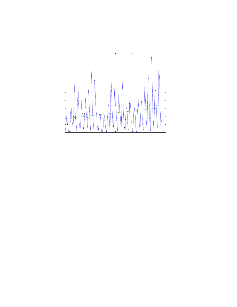
There is a slight upward trend to the data. A least squares fit gives the

trend line.

c = polyfit(t,wolfer,1);
trend = polyval(c,t);
plot(t,[wolfer; trend],’-’,t,wolfer,’k.’)
xlabel(’year’)
ylabel(’Wolfer index’)
title(’Sunspot index with linear trend’)

7

1700

1750

1800

1850

1900

1950

2000

0

20

40

60

80

100

120

140

160

180

200

year

Wolfer index

Sunspot activity

You can definitely see the cyclic nature of the phenomenon. The peaks and

valleys are a little more than 10 years apart.

Now, subtract off the linear trend and take the finite Fourier transform.

y = wolfer - trend;
Y = fft(y);

The first Fourier coefficient, Y(1), can be deleted because subtracting the linear
trend insures that Y(1) = sum(y) is zero.

Y(1) = [];

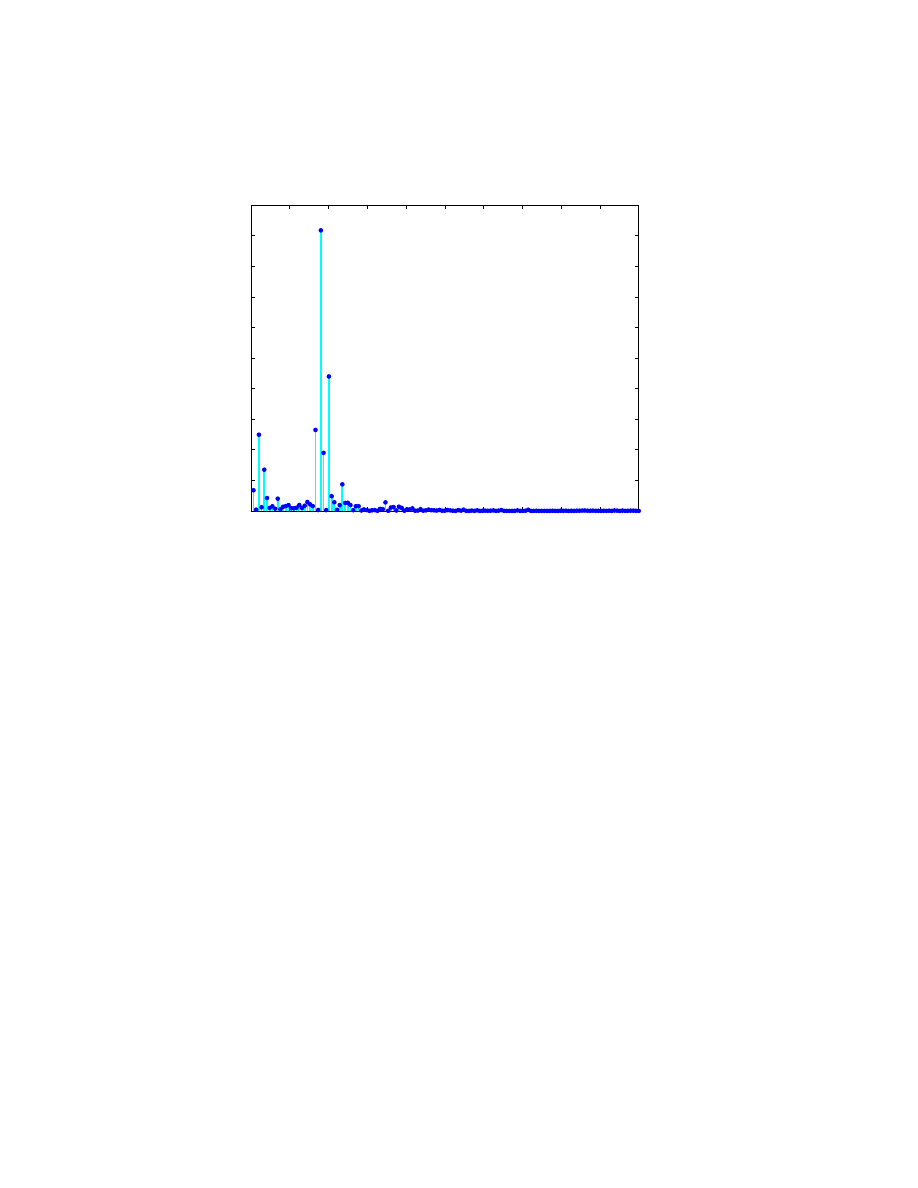
The complex magnitude squared of Y is called the power and a plot of power

versus frequency is a ”periodogram”. The frequency is the array index scaled
by n, the number of data points. Since the time increment is one year, the
frequency units are cycles per year.

pow = abs(Y(1:n/2)).^2;
pmax = 20e6;
f = (1:n/2)/n;
plot([f; f],[0*pow; pow],’c-’, f,pow,’b.’, ...

’linewidth’,2,’markersize’,16)

axis([0 .5 0 pmax])
xlabel(’cycles/year’)
ylabel(’power’)
title(’Periodogram’)

8

0

0.05

0.1

0.15

0.2

0.25

0.3

0.35

0.4

0.45

0.5

0

0.2

0.4

0.6

0.8

1

1.2

1.4

1.6

1.8

2

x 10

7

cycles/year

power

Periodogram

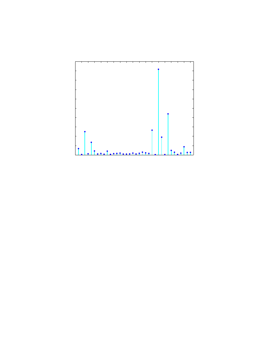
The maximum power occurs near frequency = 0.09 cycles/year. We would

like to know the corresponding period in years/cycle. Let’s zoom in on the plot
and use the reciprocal of frequency to label the x-axis.

k = 1:36;
pow = pow(k);
ypk = n./k(2:2:end);

% Years per cycle

plot([k; k],[0*pow; pow],’c-’,k,pow,’b.’, ...

’linewidth’,2,’markersize’,16)

axis([0 max(k)+1 0 pmax])
set(gca,’xtick’,k(2:2:end))
xticklabels = sprintf(’%5.1f|’,ypk);
set(gca,’xticklabel’,xticklabels)
xlabel(’years/cycle’)
ylabel(’power’)
title(’Periodogram’)

9

144.0 72.0 48.0 36.0 28.8 24.0 20.6 18.0 16.0 14.4 13.1 12.0 11.1 10.3 9.6 9.0 8.5 8.0

0

0.2

0.4

0.6

0.8

1

1.2

1.4

1.6

1.8

2

x 10

7

years/cycle

power

Periodogram

As expected, there is a very prominent cycle with a length of about 11 years.

This shows that over the last 300 years, the period of the sunspot cycle has been
slightly over 11 years.

4

Fast Finite Fourier Transform

We all use FFTs everyday without even knowing it. Cell phones, disc drives,
DVD’s and JPEG’s all involve finite Fourier transforms. One-dimensional tran-
forms with a million points and two-dimensional 1000-by-1000 transforms are
common. The key to modern signal and image processing is the ability to do
these computations rapidly.

Direct application of the definition

Y

k+1

=

n

−1

X

j=0

ω

jk

y

j+1

, k = 0, . . . , n − 1

requires n multiplications and n additions for each of the n components of Y for
a total of 2n

2

floating point operations. And that does not count the generation

of the powers of ω. A computer capable of doing one multiplication and addition
every microsecond would require a million seconds, or about 11.5 days, to do a
million point FFT.

Several people discovered fast FFT algorithms independently and many peo-

ple have since contributed to their development, but it was a 1965 paper by John
Tukey of Princeton University and John Cooley of IBM Research that is gener-
ally credited as the starting point for the modern usage of the FFT.

10

Modern fast FFT algorithms have computational complexity O(n log

2

n) in-

stead of O(n

2

). When n is a power of 2, a one-dimensional FFT of length n

requires less than 3n log

2

n floating point operations. For n = 2

20

, that’s a fac-

tor of almost 35,000 faster than 2n

2

. Even when n = 1024 = 2

10

, the factor is

about 70.

With MATLAB 5.3 and a 266 MHz Pentium laptop, the time required for

fft(x)

when length(x) is 2

20

= 1048576 is about 5 seconds. MATLAB 6.0

is still in development in February, 2000, but its new FFT code is available for
testing. With the new code, a length 2

20

fft

takes less than half a second. The

new code is based on FFTW, ”The Fastest Fourier Transform in the West”,
developed at MIT and available from http://www.fftw.org.

The key to the fast FFT algorithms is the double angle formula for trig

functions. Using complex notation and

ω = ω

n

= e

−2πi/n

= cos δ

− i sin δ

we have

ω

2

2n

= ω

n

Written out in terms of separate real and imaginary parts, this is

cos 2δ

=

cos

2

δ − sin

2

δ

sin 2δ

= 2 cos δ sin δ

Start with the basic definition.

Y

k+1

=

n−1

X

j=0

ω

jk

y

j+1

, k = 0, . . . , n − 1

Assume that n is even and that k ≤ n/2 − 1 Divide the sum into terms with
even subscripts and terms with odd subscripts.

Y

k+1

=

X

even

j

ω

jk

y

j+1

+

X

odd

j

ω

jk

y

j+1

=

n/2−1

X

j=0

ω

2jk

y

2j+1

+ ω

k

n/2−1

X

j=0

ω

2jk

y

2j+2

The two sums on the right are components of the FFTs of length n/2 of the
portions of y with even and odd subscripts. In order to get the entire FFT of
length n, we have to do two FFTs of length n/2, multiply one of these by powers
of ω, and concatenate the results.

The relationship between an FFT of length n and two FFTs of length n/2

can be expressed compactly in MATLAB. If n = length(y) is even,

omega = exp(-2*pi*i/n);
k = (0:n/2-1)’;

11

w = omega .^ k;
u = fft(y(1:2:n-1));
v = w.*fft(y(2:2:n));

then

fft(y) = [u+v; u-v];

Now, if n is not only even, but actually a power of 2, the process can be

repeated. The FFT of length n is expressed in terms of two FFTs of length n/2,
then four FFTs of length n/4, then eight FFTs of length n/8 and so on until
we reach n FFTs of length one. An FFT of length one is just the number itself.
If n = 2

p

, the number of steps in the recursion is p. There is O(n) work at each

step, so the total amount of work is

O(np) = O(n log

2

n)

If n is not a power of two, it is still possible to express the FFT of length n

in terms of several shorter FFTs. An FFT of length 100 is two FFTs of length
50, or four FFTs of length 25. An FFT of length 25 can be expressed in terms
five FFTs of length five. If n is not a prime number, an FFT of length n can
be expressed in terms of FFTs whose lengths divide n. Even if n is prime, it is
possible to embed the FFT in another whose length can be factored. We will
not go into the details of these algorithms here.

The fft function in MATLAB 5 uses fast algorithms whenever the length

is a product of small primes. The fft function in MATLAB 6 will use fast
algorithms even when the length is prime.

5

ffttx

Our textbook function ffttx combines the two basic ideas of this chapter. If n
is a power of 2, it uses the O(n log

2

n) fast algorithm. If n has an odd factor, it

uses the fast recursion until it reaches an odd length, then sets up the discrete
Fourier matrix and uses matrix-vector multiplication.

function y = ffttx(x)
%FFTTX Textbook Fast Finite Fourier Transform.
% FFTTX(X) computes the same finite Fourier transform
% as FFT(X).

The code uses a recursive divide and conquer

% algorithm for even order and matrix-vector multiplication
% for odd order.

If length(X) is m*p where m is odd and

% p is a power of 2, the computational complexity of this
% approach is O(m^2)*O(p*log2(p)).

x = x(:);
n = length(x);
omega = exp(-2*pi*i/n);

12

if rem(n,2) == 0

% Recursive divide and conquer
k = (0:n/2-1)’;
w = omega .^ k;
u = ffttx(x(1:2:n-1));
v = w.*ffttx(x(2:2:n));
y = [u+v; u-v];

else

% The Fourier matrix.
j = 0:n-1;
k = j’;
F = omega .^ (k*j);
y = F*x;

end

6

Fourier Integral Transform

The Fourier integral transform converts one complex function into another.

The transform is

F (µ) =

Z

+∞

−∞

f (t)e

−2πiµt

dt

The inverse transform is

f (t) =

Z

+

∞

−∞

F (µ)e

+2πiµt

dµ

The variables t and µ run over the entire real line. If t has units of seconds, then
µ has units of radians per second. Both functions f (t) and F (µ) are complex
valued, but in most applications the imaginary part of f (t) is zero.

Alternative units use ν = 2πµ, which has units of cycles or revolutions per

second. With this change of variable, there are no factors of 2π in the exponen-
tials, but there are factors of 1/

√

2π in front of the integrals, or a single factor

of 1/(2π) in the inverse transform. Maple and MATLAB’s Symbolic Toolbox
use this alternative notation with the single factor in the inverse transform.

7

Fourier Series

A Fourier series converts a periodic function into an infinite sequence of Fourier
coefficients. Let f (t) be the periodic function and let L be its period, so

f (t + L) = f (t) for all t

The Fourier coefficients are given by integrals over the period

c

j

=

1

L

Z

L/2

−L/2

f (t)e

−2πijt

dt, j = . . . , −1, 0, 1, . . .

13

With these coefficients, the complex form of the Fourier series is

f (t) =

∞

X

j=−∞

c

j

e

2πijt/L

8

Discrete time Fourier tranform

A discrete time Fourier transform converts an infinite sequence of data values
into a periodic function. Let x

k

be the sequence, with the index k taking on all

integer values, positive and negative.

The discrete time Fourier transform is the complex valued periodic function

X(e

iω

) =

∞

X

k=−∞

x

k

e

ikω

The sequence can then be represented

x

k

=

1

2π

Z

π

−π

X(e

iω

)e

−ikω

dω, k = . . . , −1, 0, 1, . . .

9

Finite Fourier Transform

The finite Fourier transform converts one finite sequence of coefficients into
another sequence of the same length, n.

The transform is

Y

k+1

=

n−1

X

j=0

y

j+1

e

−2ijkπ/n

, k = 0, . . . , n − 1

The inverse transform is

y

j+1

=

1

n

n

−1

X

k=0

Y

k+1

e

2ijkπ/n

, j = 0, . . . , n − 1

10

Connections

The Fourier integral transform involves only integrals. The finite Fourier trans-
form involves only finite sums of coefficients. Fourier series and the discrete
time Fourier transform involve both integrals and sequences. It is possible to
”morph” any of the systems into any of the others by taking limits or restricting
domains.

Start with Fourier series. Let L, the length of the period, become infinite and

let j/L, the coefficient index scaled by the period length, become a continuous
variable, µ. Then the Fourier coefficients, c

j

, become the Fourier transform,

F (µ).

14

Again, start with Fourier series. Interchanging the roles of the periodic func-

tion and the infinite sequence of coefficients leads to the discrete time Fourier
transform.

Start with Fourier series a third time. Now restrict t to a finite number of

integral values, k and restrict j to the same finite number of values. Then the
Fourier coefficients become the finite Fourier transform.

In the Fourier Integral context, Parseval’s theorem says

Z

+∞

−∞

|f(t)|

2

dt =

Z

+∞

−∞

|F (µ)|

2

dµ

This quantity is known as the total power in a signal.

Exercises

1. (el Ni˜

no) The climatological phenomenon el Ni˜

no results from changes in

atmospheric pressure in the southern Pacific ocean. The ”Southern Oscilla-
tion Index” is the difference in atmospheric pressure between Easter Island and
Darwin Australia, measured at sea level at the same moment. The text file
elnino.dat

contains values of this index measured on a monthly basis over the

14 year period 1962 through 1975.

Your assignment is to carry out an analysis similar to the sunspot example

on the el Ni˜

no data. The unit of time is one month instead of one year. You

should find there is a prominent cycle with a period of 12 months and a second,
less prominent, cycle with a longer period. This second cycle shows up in about
three of the Fourier coefficients, so it is hard to measure its length, but see if
you can make an estimate.

2. (Train signal) The MATLAB demos directory contains several sound samples.
One of them is a train whistle. The statement

load train

will give you a long vector y and a scalar Fs whose value is the number of
samples per second. The time increment is 1/Fs seconds.

If your computer has sound capabilities, the statement

sound(y,Fs)

will play the signal, but you don’t need that for this problem.

The data does not have a significant linear trend. There are two pulses of

the whistle, but the harmonic content of both pulses is the same.

(a) Plot the data with time in seconds as the independent variable.
(b) Produce a periodogram with frequency in cycles/second as the indepen-

dent variable.

(c) Identify the frequencies of the six peaks in the periodogram. You should

find that ratios between these six frequences are close to ratios between small

15

integers. For example, one of the frequencies of 5/3 times another. The fre-
quences that are integer multiples of other frequencies are ”overtones”. How
many of the peaks are fundamental frequencies and how many are overtones?

16