• SO&P, D15: Report on the interpretation of palaeodata using climate simulations

Representing Simulations by Reconstructions

Gerd Bürger, FU Berlin

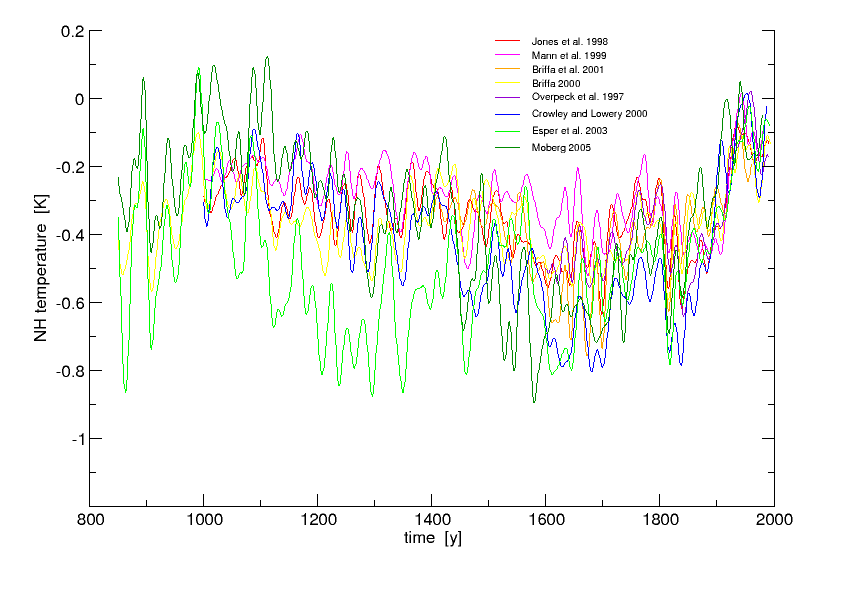
During the SO&P project phase one was faced with a growing number of attempts to reconstruct millennial NH temperatures from various sources of proxy information (Jones et al., 1998; Mann et al., 1999; Briffa et al., 2001; Briffa, 2000; Overpeck et al., 1997; Crowley & Lowery, 2000; Esper et al., 2002; Moberg, 2005). These attempts did not show, however, converge towards a unique millennial history, as shown in Fig. 1. Note that the proxy series have already undergone a linear transformation towards a best estimate to the CRU data (which makes them look more similar, cf. Briffa and Osborn, 2002).

Figure 1. Eight recent proxy based NH (> 20N) temperature reconstructions. A 10y Butterworth filter was used for smoothing.

At the same time, a series of millennial climate simulations was conducted using estimates of solar irradiance (S), greenhouse gases (G), and volcanic aerosols (V) as external historical forcing. Ideally, the internal (=natural) fluctuations (the “noise”) as well as the forcing response (the “signal”) is of the same scale (and shape) in all models and equals reality. And with a sufficiently large signal-to-noise ratio (SNR) for a given forcing it should be possible to distinguish the signal from the noise and determine the sensitivity of the climate system to that forcing; moreover, proxies and models would show the same signal. In the real world, however, both noise and signal tend to depend on the specific model, and since proxy reconstructions are imperfect as well the real signal is deeply obscured.

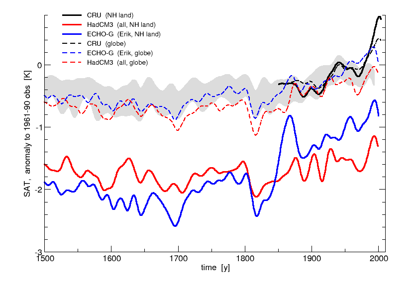
Fig. 2 shows two millennial simulations using all three forcings (S, G, and V), one from the Hadley centre model HadCM3 (“all” simulation) and the other from the DKRZ model ECHO-G (“Erik” simulation). Obviously both models deviate considerably from each other and from the instrumental record (Jones et al., 1999), with a cold bias of as much as 1K (ECHO-G) and 1.5K (HadCM3). This is compensated for by a tropical and SH warm bias (not shown) which gives a much better fit for the global average. At least some of the Northern Hemisphere difference between the two simulations may be because the HadCM3 all simulation has aerosol forcing, whereas the Erik simulation does not (Note that GCM parameters are tuned using that average, among others, as a target.) It is unlikely that from those raw time series a forcing signal can be detected.

Figure 2. Observed and simulated annual mean temperature anomalies over land (smoothed) using the available points from the observational grid, relative to the 1961-90 observed mean. Black: CRUTEM2v; blue: ECHO-G; red: HadCM3. Dashed: Global land/ocean. Grey: range of reconstructions (cf. Fig.1).

However, under rather mild assumptions it can be assumed that the response of the system will not change drastically if transfered from the too cold to the normal state. Therefore, it is justified to replace both simulations with a corresponding best estimate to the CRU data, just like the proxies in Fig. 1.

The best-estimate transformation moreover provides a compact way to interpret the paleo series in the light of the climate simulations. Regressing, in a multivariate way, the latter on the former yields for each simulation and reconstruction a corresponding regression coefficient, as shown in Table 1 (along with corresponding correlations). From this it appears that the ECHO-G simulation better fits the proxies, with a multiple correlation of 0.78 compared to 0.48 for the HadCM3. The regression of the latter is equally dominated by the Crowley/Lowery and Briffa 2000 reconstruction, while the ECHO-G regression is almost completely determined by Crowley/Lowery. This is probably due to their common long term millennial cooling and then sharp warming trend, with a correlation of 0.72.

	HadCM3		ECHO-G
	regr. coef.	corr.	regr. coef.	corr.
Jones et al. 1998	0.05	0.35	-0.06	0.40
Mann et al. 1999	0.12	0.29	0.04	0.39
Briffa et al. 2001	-0.01	0.30	0.24	0.47
Briffa 2000	0.19	0.37	0.16	0.42
Overpeck et al. 1997	0.01	0.45	-0.27	0.62
Crowley and Lowery 2000	0.21	0.44	0.80	0.72
Esper et al. 2003	-0.04	0.40	0.03	0.39
Moberg 2005	0.03	0.32	0.15	0.65
multiple correlation	0.48		0.78

Table 1.: Regression and correlation coefficients for the Northern Hemisphere land temperature anomalies for the two simulations regressed onto proxy based Northern Hemisphere temperature reconstructions..

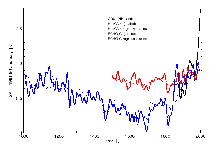
The regression creates a best fit of the reconstructions to each simulation, as shown in Fig. 3. Note that also on the smaller (decadal) time scales ECHO-G shows greater covariability with the reconstructions. As a result, the Spörer, the Maunder and the Dalton minima are clearly visible. Larger deviations are seen in the early 12th and late 19th century where the ECHO-G simulates much warmer conditions than the reconstructions.

Figure 3. Observed (CRU, black) and simulated NH temperatures (best estimate to CRU; red: HadCM3, blue: ECHO-G), along with its regression on proxies (thin lines). 10y smoothing.

• References

Briffa, K. R., and Osborne, T., 2002: Blowing hot and cold. Science, 295, 2227-2228.

Jones, P. D., New, M., Parker, D. E., Martin, S. and Rigor, I. G., 1999: Surface air temperature and its variations over the last 150 years. Reviews of Geophysics 37, 173-199.

Jones, P. D., Briffa, K. R., Barnett, T. P. and Tett, S. F. B., 1998. High-resolution palaeoclimatic records for the last millennium: interpretation, integration and comparison with General Circulation Model control-run temperatures. The Holocene 8(4), 455-471.

Mann, M. E., Bradley, R. S., and Hughes, M. K., 1999. Northern Hemisphere Temperatures During the Past Millennium: Inferences, Uncertainties, and Limitations. GRL, Vol. 26, No. 6, p.759.

Briffa, K. R., Osborn, T. J., Schweingruber, F. H., Harris, I. C., Jones, P. D., Shiyatov, S. G. and Vaganov, E. A., 2001. Low frequency temperature variations from a northern tree-ring density network. J. Geoph. Res., 106, 2929-2941.

Briffa, K. R., 2000. Annual climate variability in the Holocene: intepreting the message of ancient trees. Quat. Science Rev., 19, 87-105.

Overpeck, J., K. Hughen, D. Hardy, R. Bradley, R. Case, M. Douglas, B. Finney, K. Gajewski, G. Jacoby, A. Jennings, S. Lamoureux, A. Lasca, G. MacDonald, J. Moore, M. Retelle, S. Smith, A. Wolfe, and G. Zielinski, 1997. Science, 278, 1251-1256.

Crowley, T. J., and T. Lowery, 2000. How Warm Was the Medieval Warm Period? Ambio, 29, 51-54.

Esper, J., E. R. Cook, and F. H. Schweingruber, 2002. Low-frequency signals in long tree-line chronologies for reconstructing past temperature variability. Science, 295, 2250-2253.

Moberg, A., Sonechkin, D. M., Holmgren, K., Datsenko, N. M. and Karlen, W., 2005. Highly variable Northern Hemisphere temperatures reconstructed from low- and high-resolution proxy data. Nature 433, 613-617.

---