Wytrzymałość Materiałów 3

Zadanie 4

Dla belki dwupodporowej z wysięgnikami podanej na

rys.14, obliczyć wartości reakcji R_Ax, R_Ay oraz R_B, a także podaj

przebieg sił wewnętrznych. Obciążenie belki jest podane

w tabeli:

Tabela

i	xi m	Pi kN	αi rad	Mi kNm
1	0	1	π/3	1
2	3	2	7π/6	-2
3	9	5	π/4	1
4	12	√2	π/4	1

Obliczenie wartości sił reakcji: dla α_B = π /3

z równania (d) otrzymujemy

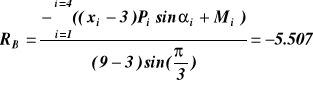
kN

równania (e) i (f) dają: R_Ax = −0.550 kN, R_Ay = 0.368 kN

R_Ay R_B

P₁ M₂ α_B P₄

M₁ α₁ α₂ R_Ax M₃ P₃

α₃ 4 α₄

1 x

P₂ 2 3 M₄

x₂=a

x₃=b

x₄ = l

Rys. 14 Belka na dwóch podporach

Analiza sił wewnętrznych 15WM

- w przedziale 0≤ x≤ 3

P₁

M_x

M₁ α₁ N

1 x

x T Rys.14a

∑P_x = P₁cosα₁ + N = 0 N = - P₁cosα₁

∑P_y = P₁sinα₁ - T = 0 T = P₁sinα₁

∑M_i = M₁ - P₁sinα₁x + M_x = 0

- w przedziale 3≤ x≤ 9

R_Ay

P₁ M₁ M₂

M₁ α₁ α₂ R_Ax

N x

P₂ A M_x

a T

x Rys.14b

∑P_x = P₁cosα₁ + P₂cosα₂ + R_Ax + N = 0

∑P_y = P₁sinα₁ + P₂sinα₂ + R_Ay - T = 0

∑M_i = M₁ - M₂ - P₁sinα₁x - P₂sinα₂ (x-a) + M_x = 0

- w przedziale x≥ 9

P₄

M_x T 4 α₄

N x

l - x M₄ Rys.14c

∑P_x = P₄cosα₄ - N = 0 ∑P_y = P₄sinα₄ + T = 0

∑M_i = M₄ + P₄sinα₄ (l-x) -M_x = 0

Wykresy sił wewnętrznych 16WM

T kN

0.866

0.230

0 x

1.78 -1.0

N kN

1.0

x

-0.50 5.0

M_x kNm 4.0

3.6

1.6

1.0

x

-1.0 Rys.14d

Naprężenia przy czystym zginaniu

P a A B a P

R_A R_B

M_g=Pa

T=P T = 0

T = P

Rys. 15 Realizacja czystego zginania

O 17WM

ρ - ro d* z

ρ ρ -z s

A B A B

s₁ z z₂

s x x

D C z₁

D C

Rys. 13 Określenie odkształceń względnych

s = ρd*, s₁ = (ρ - z)d*

(7)

Z prawa Hooke^'a mamy: * = Eε = -Ez ρ (8)

x

z

M = M_y

M_z = 0

T = 0

z₂ N = 0

z x

y

- z₁

M_y y

Rys.17 y oś obojętna, * = 0

Rys.17a, obraz rzeczywistego stanu naprężeń Rys.17a

Określenie położenia osi obojętnej 18WM

1) z warunku N = 0

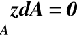
wniosek oś y (oś obojętna) jest osią przechodzącą przez środek ciężkości taka oś nazywa się

osią centralną takich osi jest nieskończona ilość

2) M_Z = 0

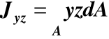
odśrodkowy moment bezwładności

Jeśli J_yz = 0 to osie y,z nazywamy osiami głównymi,

jeśli te osie przechodzą przez środek ciężkości przekroju to nazywamy je osiami głównymi centralnymi.

3)
M_y = M_g

(8a)

mnożymy i dzielimy (8a) przez z oraz przez (-1)

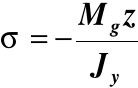
(9)

Przykład 5

Wyznaczyć średnicę d środkowej części osi wagonu (rys.18) aby ekstremalne naprężenia spełniały warunek *_e ≤ 75 MPa.

1845 Z symetrii układu R₁ = R₂

P a P oznaczmy R₁ = R₂ = R

a-a

a z z_max

R₁ 1435 R₂ M_g=Pb

P = 60kN b = (1845-1435) 2 = 205mm y

Rys.15 Do zadania 5

Rozwiązanie d

Aby określić z wzoru (9) wartość średnicy wału

należy znać wzór na J_y pola przekroju kołowego.

Wyprowadzenie wzoru.

z dF = dsdr = rd*dr

*

z=r sin*

x

dr Rys.16

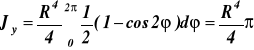
(10)

z wzoru (9) mamy :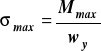
(10a)

gdzie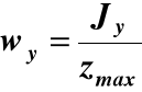
wskaźnik wytrzymałości

dla przekroju kołowego pełnego

Z wzoru (10a) i warunku że *_max = *_e = 75MPa mamy:

Linia ugięcia belki 20WM

Z wzoru (8a) mamy 1 ρ = M_g(x) EJ_y

w(x) ρ P

ϑ

A x

x w_x

l

Rys.16 Określenie ugięć belki (w przekroju A belka

zamurowana)

Z geometrii różniczkowej wiemy, że krzywizna 1 ρ linii

w(x) wyraża się wzorem

1 ρ = w^'' (1 + w^'2)^3/2 dla małych w^' 1 ρ = w^'' i wtedy:

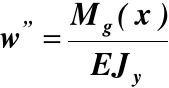
(11)

Przykład 6

Wyznaczyć linię ugięcia pryzmatycznej belki (rys.16) o przekroju kołowym. Określić ekstremalny kąt ugięcia ϑ_e i ekstremalne ugięcie

w_e = f, tzw. strzałkę ugięcia.

Przyjąć, że P = 10kN, l =1m, E = 2*10⁵ MPa, a dopuszczalne naprężenie k_r = k_c = 100MPa

Rozwiązanie

M_g =P(l-x) dla 0* x * l

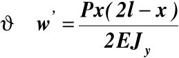
po scałkowaniu równania (11) otrzymujemy:

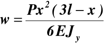
Całkując powyższe wyrażenie mamy:

Stałe całkowania wyznaczamy z warunków brzegowych:

w_x=0 = 0; w^'_x=0 = 0 stąd C = 0; D = 0 w efekcie mamy:

(a)

Dla x = l

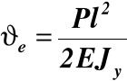
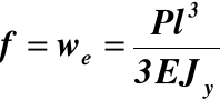
(12)

Po podstawieniu danych liczbowych do wzorów (12)

*_e =0.29⁰ f = 3.4mm

Jak widać (f /l) jest tu rzędu 1/300.

14WM

M z *

y

d*

r

R

19 WM

21WM

---