© 2011 ANSYS, Inc.

January 16, 2012

1

Release 14.0

14. 0 Release

Introduction to ANSYS
CFX

Lecture 06
Day 1 Review and Tips

© 2011 ANSYS, Inc.

January 16, 2012

2

Release 14.0

Introduction

•

Lecture Theme:

–

The focus of Day 1 has been to cover topics (defining material properties, defining 
boundary and cell zone conditions, running the simulation, post‐processing the 
results) which include operations that are common to any CFD analysis in CFX.

–

Many analyses will require additional inputs, such as turbulence models or system 
rotation,  will be the focus of Day 2. 

•

Learning Aims – you have learned:

–

Boundary conditions, cell zone conditions and material properties

–

Post‐processing

–

Solver settings

•

Learning Objectives:

–

After Day 1, you will be able to set up, run and post‐process your own CFD 
simulation

Introduction

Problem Definition

Running Simulation

Post‐processing

Summary

© 2011 ANSYS, Inc.

January 16, 2012

3

Release 14.0

Before you Start CFX

•

Define your modelling goals

•

Identify the computational domain

–

Simplify if possible

–

Think about where boundary conditions can be set

–

Avoid placing boundaries in potential recirculation areas when possible

•

Create / Import the Geometry

–

Consider meshing requirements when creating the geometry

–

Do not include unnecessary detail

•

Create a suitable mesh

–

Resolve expected gradients in the solution variables

–

Check mesh quality metrics

Introduction

Problem Definition

Running Simulation

Post‐processing

Summary

© 2011 ANSYS, Inc.

January 16, 2012

4

Release 14.0

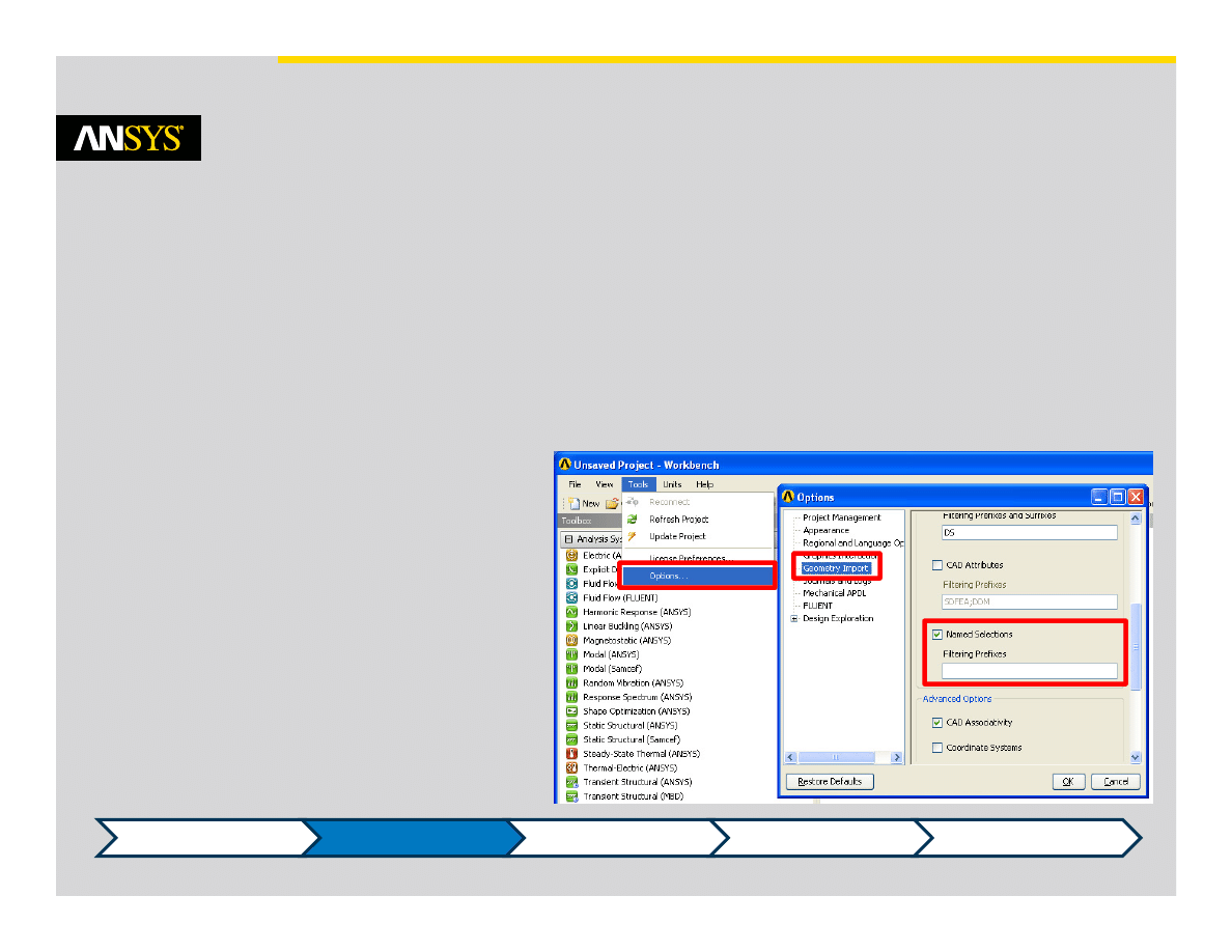
Working with Workbench

•

Save your Project to set the working directory

•

Create the workflow by dragging and dropping Analysis and Component 
Systems onto the Project Schematic

–

Systems can share or transfer data by dropping onto an appropriate cell

•

Configure Tools > Options to suit your needs

–

E.g. Enable Named Selections
and blank the Filter to always
pass Named Selections from
the Geometry to the Mesh

Introduction

Problem Definition

Running Simulation

Post‐processing

Summary

© 2011 ANSYS, Inc.

January 16, 2012

5

Release 14.0

Domains

•

Domains define a region of consistent materials and physical models

•

Use different domains for:

–

Different reference frames, e.g. rotating, stationary

–

Different domain types – fluid, solid, porous

–

Different materials, e.g. oil, copper and water

•

Fluid domains that are connected should use consistent physics

•

All regions that have the same physics can be grouped into a single domain

–

Regions do not have to be connected

–

Mesh does not have to be continuous

•

The Reference Pressure should be set to the operating pressure of the 
device

Introduction

Problem Definition

Running Simulation

Post‐processing

Summary

© 2011 ANSYS, Inc.

January 16, 2012

6

Release 14.0

Boundary Conditions

•

It is important to consider the accuracy of the boundary conditions

–

E.g. a uniform velocity profile is usually not realistic, but can be used if placed a 
suitable distance upstream

•

Avoid setting boundary conditions in recirculation zones if possible

•

Use well posed boundary conditions

–

Mass Flow or Velocity Inlet, Static Pressure Outlet
• Will give a uniform inlet velocity profile

–

Total Pressure Inlet, Mass Flow Outlet
• Will allow an inlet velocity profile to develop

–

Total Pressure Inlet, Static Pressure Outlet
• Will allow an inlet velocity profile to develop

Introduction

Problem Definition

Running Simulation

Post‐processing

Summary

© 2011 ANSYS, Inc.

January 16, 2012

7

Release 14.0

Solver Settings

•

A good initial guess will assist with Solver stability during the first few 
iterations

•

The timestep is an important solver control

–

Smaller Timestep = More Stable, but slower convergence

–

Larger Timestep = Faster convergence, but too large will cause the solver to fail

•

When the solver finishes check:

–

Residuals are converged to at least RMS 1e‐4

–

Imbalance are below 1%

–

Monitor Points for quantities of interest have reached steady values

Introduction

Problem Definition

Running Simulation

Post‐processing

Summary

© 2011 ANSYS, Inc.

January 16, 2012

8

Release 14.0

Post‐Processing

•

Automate post‐processing through Session files, State files and Report 
templates

•

Make use of Expressions and User Variables to extract engineering data

•

Compare solutions using the Multi‐file mode and the Case Comparison 
tools

•

Save images in the 3D CFX Viewer format to provide management or your 
customers with a better understanding of the flow

Introduction

Problem Definition

Running Simulation

Post‐processing

Summary

© 2011 ANSYS, Inc.

January 16, 2012

9

Release 14.0

Summary

•

Remember to first think about what the aims of the simulation are prior to 
creating the geometry and mesh

•

All CFD simulations involve some common operations

–

Problem definition

–

Defining boundary conditions and cell zone conditions

–

Defining material properties

–

Post‐processing the results

•

Use residual monitors, flux balances and solution monitors to judge 
convergence

–

Unconverged results can be misleading

•

What Next:

•

Day 2 will focus on physical models and best practices

Introduction

Problem Definition

Running Simulation

Post‐processing

Summary