A

B

C

D

E

L

1

2

1

2

L

H



H

H

x(t)

~

piston generator

Z

2

1

Z

a

b

b

1

2

a

XV Konferencja Naukowa - Korbielów’ 2003

„Metody Komputerowe w Projektowaniu i Analizie Konstrukcji Hydrotechnicznych”

Standing waves of finite amplitude in water

of non-uniform depth

Kazimierz Szmidt

1

1.

INTRODUCTION

In analysing water structure interaction problems we have to solve boundary conditions

on a wetted surface of a structure which in general is a moving surface. The simplest case in
this field seems to be a rigid breakwater, not moving in space, with a wetted surface
changing in time. An example of the letter case is a breakwater constructed in the form of a
rigid vertical wall immersed in fluid of constant depth loaded with water waves. In many
practical cases we also meet cases with sloping bottom in the vicinity of the breakwater
structure, and thus, in analysis of the latter a change of water depth should be taken into
account. Frequently, in real conditions, one may observe that water waves approaching the
breakwater have a relatively big height, often changing in time. In describing the latter cases
a finite amplitude of the waves must be also taken into account. In describing the
aforementioned problems we usually apply the space variables and time (Eulerian
description). With these variables, the fundamental equation describing the irrotational
motion of an inviscid incompressible fluid assumes the form of the Laplace equation for a
velocity potential. The main difficulty of a solution of the equation is to solve the initial and
boundary conditions of the problem considered.

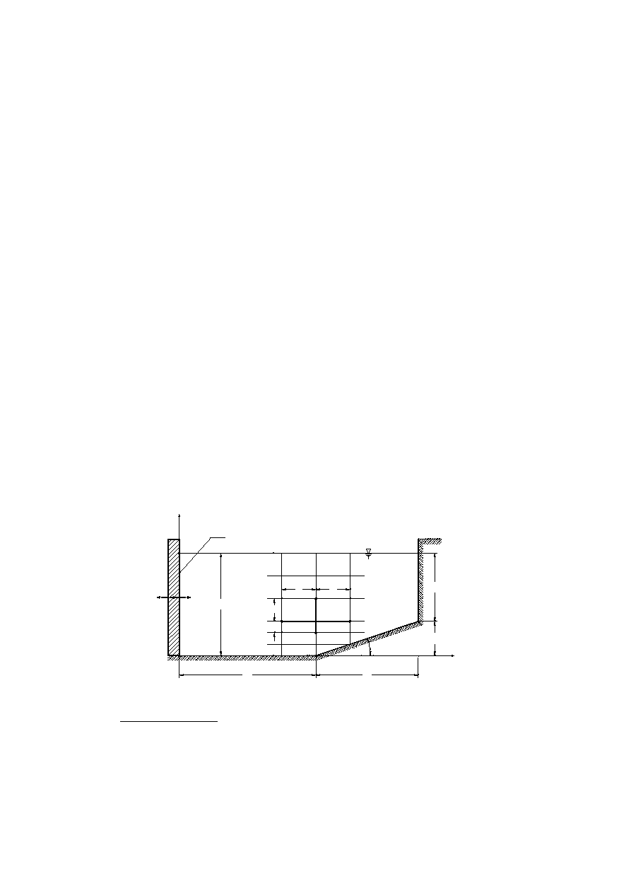
Fig. 1. Definition sketch.

1

Prof. dr hab. inż., Institute of Hydro-Engineering of PAS, ul. Kościerska 7, 80-953 Gdańsk

1

There are also regions of our interest however where a more preferable is to use the material
(Lagrangian) description, which allows us to simplify the solution of the boundary
conditions on a moving boundary of the fluid domain. In particular, the Lagrangian
variables are more convenient in calculating the hydrodynamic interaction of the fluid and
structure. In this paper we confine our attention to the material description of the initial
value problem of fluid being at rest and starting to move at a certain moment of time.
Following the problems mentioned above we will consider an approximate solution to the
problem of water waves of finite amplitude reflected from a rigid vertical boundary.

2.

FORMULATION OF THE PROBLEM

The theoretical model considered is shown schematically in Fig.1. The waves are

generated by a piston type generator forming the left boundary of the domain. Due to
reflection from the right boundary (the vertical wall CD in the figure) we have the case of
standing waves in the fluid domain. The frequency of the generation was chosen to be equal
to the resonance frequency of the fluid domain. In this way a standing wave of finite
amplitude
growing in time on the right boundary is obtained. The case considered corresponds to
smooth waves sufficiently far off breaking. In what follows we confine our attention to the
plane problem of a fluid motion in the Euclidean space. Fundamental relations of the
problem considered may be found in Szmidt (2001). To make the discussion clear some of
the important results obtained in the work are summarized below. In order to describe the
fluid motion we introduce the Cartesian coordinate system

)

2

,

1

,

(



r

z

r

in the actual

configuration. In the reference configuration, the Cartesian coordinates, corresponding to
names of the fluid particles, are denoted by

)

2

,

1

,

(







Z

. Moreover, it is convenient to

introduce a common Cartesian coordinate system. The motion of the fluid is described by
the mapping of the names into the positions occupied by the material points at the time

0



t

)

,

(

)

,

(

t

Z

w

Z

t

Z

z

i

i

i















,

(1)

where

i





is the Kronecker’s delta and

i

w

are components of the displacement vector.

The Jacobian of the transformation is the determinant of the matrix of the transformation
gradient

 

i

z

J





,

det

,

(2)

where the symbol



,

denotes the partial derivative with respect to



Z

. In a similar way

,

the symbol

i

,

denotes the partial derivative with respect to

i

z

, and the subscript

t

,

means

the partial derivative with respect to time. For the discussed, two – dimensional case, the
inverse of the matrix of the transformation gradient reads

 

























1

1

,

2

1

,

1

2

,

2

2

,

,

1

z

z

z

z

J

Z

i

,

(3)

2

where the subscripts mean the partial derivatives with respect to the material variables



Z

for

2

,

1





.

Knowing the above relations we may transform important formulae from the Eulerian
variables into the Lagrangian variables and vice versa. Thus, let us consider the potential
function

)

,

(Z t





expressed in terms of the material variables. In these variables the

Laplace equation assumes the following form





0

,

,

,

,















r

s

rs

Z

Z

.

(4)

With respect to the potential, the velocity components are

,

)

,

(

,











r

r

Z

t

Z

w

(5)

where the dot denotes the material time derivative.
In the discussed case the fluid density is constant and the Jacobian of the mapping

)

,

(

t

Z

z

z

i

i





is equal to one. Accordingly, in what follows it is convenient to introduce

the “pressure” function

)

(

2

1

)

,

(

,

,

,

,

t

C

Z

Z

h

p

t

Z

P

s

r

rs



































.

(6)

where

)

(t

C

is a “constant” of the solution, and

h

is the potential of the mass force due to

the gravitational field. In the spatial description the potential is given by the relation

3

)

(

gz

z

h

r



,

(7)

where the coordinates are chosen in such a way that

3

z

acts vertically upwards and

g

is

the gravitational acceleration

.

For the considered two-dimensional problem one may

introduce the classical notation

y

z

x

z





2

1

,

for the actual configuration and

Y

Z

X

Z





2

1

,

for the reference configuration. With respect to this notation Eq (5)

gives

).

1

(

,

)

1

(

,

,

,

,

2

,

,

,

,

1

X

Y

Y

X

X

Y

Y

X

u

u

v

w

v

v

u

w



































(8)

Having the velocity we may calculate the displacement components

.

)

0

,

(

)

,

(

)

,

(

),

0

,

(

)

,

(

)

,

(

0

0





































t

Z

v

d

Z

v

t

Z

v

t

Z

u

d

Z

u

t

Z

u

t

t





(9)

3

In order to describe the initial and boundary conditions, let us consider the case shown in
Fig. 1. The motion of the fluid is induced by the piston-type wavemaker (the rigid wall AE
in the figure) starting to move at a certain moment of time. For the case shown in Fig 1 the
boundary conditions are:

.,

)

,

(

d)

,

0

)

,

0

(

c)

,

0

)

,

(

b)

),

(

)

,

0

(

a)

2

2

1

0

1

const

t

H

Z

P

t

Z

v

t

L

Z

u

t

x

t

Z

u

















,

(10)

where

)

(

0

t

x

describes the horizontal displacement of the wall AE in the figure, and the

constant in Eq (10d) will be assumed equal to zero. In the further part we will consider the
initial value problem of the fluid motion starting from rest.

3.

GENERATOR MOTION

Let us consider the piston type generator starting to move at a certain moment of time.

It is assumed a smooth beginning of the fluid motion for which not only the velocity, but
also the acceleration field disappear at the initial moment of time. The motion of the
generator is assumed in the following form (Wilde and Wilde, 2001)

t

D

t

A

a

t

x















sin

)

(

cos

)

(

)

(

0

,

(11)

where



is the angular frequency,

3



 s

a

and

,

),

exp(

!

3

1

!

2

1

1

1

)

(

),

exp(

!

3

1

)

(

3

2

3

t

D

t

A

















































(12)

where



is a parameter.

One may check that the displacement together with its first and second derivatives are equal
to zero at the starting point. Moreover, with passing time, the generation goes
asymptotically to harmonic displacement with constant amplitude. In the further discussion
we confine our attention to generation described by the latest formulae. The non-linear
problem at hand has no closed analytical solution and therefore, in order to find a solution
of it, we

have to approximate the fundamental equations by ones which are more tractable.

One of the methods of approximation is the infinitesimal - wave approximation based on a
perturbation procedure (Wehausen and Laitone, 1960) in which functions entering the
problem are expanded into power series in a small parameter.

4. SMALL PARAMETER REPRESENTATION OF THE FUNDAMENTAL

RELATIONS

Let us consider the equation of motion together with appropriate boundary and initial

conditions. The functions entering the equations are expanded in a small parameter



.

4

Thus, we have

.

)

,

(

,

)

,

(

,

)

,

(

3

3

2

2

1

3

3

2

2

1

3

3

2

2

1





































































v

v

v

t

Z

v

u

u

u

t

Z

u

t

Z

(13)

where

i



,

i

u

and

i

v

for







,

3

,

2

,

1

i

are “components” of the solutions.

In what follows we confine our attention to the second order expansion. Substituting these
expressions into Eq (4) and collecting terms with the same powers in



, one finds









0,

2

,

0

1

1

,

1

22

,

1

1

,

1

2

,

1

12

,

1

2

,

1

,11

2
,22

2

11

,

2

1

22

,

1

11

,









































u

v

u

v

(14)

where the terms up to the second order are displayed.
It is seen the linear component of the expansion results in the Laplace equation for the
velocity potential

)

,

(

1

t

Z





identical to that one in the space variables, while for the

higher component we have the Poisson’s equation. Therefore, in constructing the first order
solution for the velocity potential

)

,

(

1

t

Z





we do not need to distinguish the co-ordinate

systems. In a similar way, the expansion of the velocity components reads









.

)

,

(

,

)

,

(

1

2

,

1

1

,

1

1

,

1

2

,

2

2

,

2

1

2

,

1

1

,

1

2

,

1

2

,

1

1

,

2

1

,

2

1

1

,

u

u

t

Z

v

v

v

t

Z

u





























































(15)

Knowing that





)

,

(

)

,

(

)

,

(

3

3

t

Z

v

Z

g

t

Z

gz

t

Z

h













, (16)

we may assume

gH

C



in Eq (6) and write

































s

r

rs

Z

Z

t

Z

t

Z

gv

Z

H

g

t

Z

P

,

,

,

,

3

2

1

)

,

(

)

,

(

)

(

)

,

(



.

(17)

The first term on the right hand side of the equation means the hydrostatic pressure

)

(

3

0

Z

H

g

P





. The pressure function may be thus rewritten as

2

2

1

0

P

P

P

P











,

(18)

5

where





.

)

(

)

(

2

1

,

2

1

2

,

2

1

1

,

2

2

2

1

1

1





























gv

P

gv

P

(19)

With respect to the expansion (18) we can write the sequence of the dynamic boundary
conditions on the upper boundary. From the first of Eq (19) it follows

0

)

,

,

(

)

,

,

(

1

1

1

1







t

H

Z

t

H

Z

gv



.

(20)

Calculating the partial time derivative of the equation one obtains

0

2

1

2

,

1









H

Z

g





.

(21)

A similar procedure for the square term (the second equation in the relations 19) gives









.

0

2

1

2

,

1

2

,

1

1

,

1

1

,

1

2

,

1

1

,

1

1

,

1

2

,

2

2

,

2

2

































H

Z

u

u

g

g









(22)

The boundary condition on the bottom A-B (

0

2



Z

) leads to the result

.

0

,

0

,

0

,

0

0

1

2

,

1

1

,

1

1

,

1

2

,

2

2

,

0

2

0

1

2

,

0

1

2

2

2

2

































Z

Z

Z

Z

u

u

v

v





(23)

On the slope B-C the normal component of the velocity equals zero, and thus

,

0

cos

1

cos

sin

,

0

cos

sin

1

,

1

1

,

2

2

,

2

1

,

1

2

,

1

1

,









































BC

t

BC

dt

(24)

where the co-ordinate axes (



,

) are defined by the line B-C and the normal vector of it.

On the vertical wall

0

1



Z

we have the condition, that the normal component of the

velocity field is equal to the velocity

)

(

0

t

x

of the generator. From the first of Eq. (15) it

follows

.

0

),

(

0

1

1

,

1

2

,

1

2

,

1

1

,

2

1

,

0

0

1

1

,

1

1





















Z

Z

v

v

t

x

(25)

6

In a similar way, on the right boundary

L

Z



1

we have

.

0

,

0

1

1

1

1

,

1

2

,

1

2

,

1

1

,

2

1

,

1

1

,





















L

Z

L

Z

v

v

(26)

5.

FD FORMULATION OF THE PROBLEM

In order to find a solution of the problem discussed we resort to discrete formulation of

it by means of the finite difference method. With this method a finite number of nodal
points of an assumed net is considered. For the domain of fluid shown in Fig.1 a non-
homogeneous spacing of points is assumed in which the spacing of vertical lines is equal to

a

while the spacing of horizontal lines is equal to

1

b

in the lower part, and

2

b

in the upper

part of the fluid domain, respectively. The assumed discrete model is shown in Fig. 1. The
differential equations for the components of the velocity potential are substituted by the
finite difference equations at all nodal points of the assumed net. To save the place we shall
use the notation



for the first order velocity potential

)

,

(

1

t

Z





. For a typical nodal

point

)

,

( j

i

within the lower part the fluid domain, where

i

means the number of a vertical

line and

j

denotes the number of a horizontal line, the finite difference representation of

the Laplace equation reads

0

,

1

1

1

,

,

1

1

,

,

1

1



































j

i

j

i

j

i

j

i

j

i

K

,

(27)

where





)

1

(

2

and

1

1

2

1

1











K

a

b

(28)

For a typical point

)

,

( j

i

within the upper part of the domain the relevant equations are

similar, but now, instead of

1

b

one should introduce

2

b

, and at the same time,

2



and

2

K

, respectively. In order to write the equations for points where the vertical dimension of

the mesh are changed the Taylor expansion has been applied.

The equations (27) are written for all nodal points of an assumed net, including

boundary points. At the same time, it should be noted that the boundary conditions of the
problem at hand involve not only the values of the potential but also the first and second
time derivatives as well as the derivatives with respect to the material co-ordinates of the
function. In order to perform integration of the equations in the time domain we resort to di-
screte description of the time, i.e. instead of the continuous time we introduce a sequence of
time steps with the increment

0



t

. In the discrete time domain in constructing an ap-

proximate solution to the boundary value problem it is convenient to use the Wilson



me-

thod which enables us to establish algebraic equations of the problem mentioned on a com-
mon level of the discrete time. The method is based on a linear approximation of an acce-
leration vector at every point of the discrete time (Bathe, 1982). In the

discussed problem of

7

the potential motion of the fluid, in place of the acceleration we

are dealing with the second

time derivatives of the potential function.

6.

THE FIRST ORDER SOLUTION

The first order solution of the problem mentioned is similar to a linear solution of the

potential flow in the Eulerian variables. In both cases we have to solve the classical Laplace
equation within the fluid domain together with appropriate initial and boundary conditions.
In constructing the solution we do not need to distinguish the co-ordinate system. Thus, we
have the following system of equations:

-

the Laplace equation

0

2

1

2

2

1

2

1

2























y

x

,

(29)

- the boundary conditions

,

0

,

0

),

(

1

1

1

0

0

1







































E

D

D

C

B

A

x

y

g

n

t

x

x







(30)

and initial conditions at



 0

t

that the displacement, velocity and acceleration field in the

fluid domain equal zero. In order to find a set of solutions of the problem at a sequence of
time steps we apply the formulae derived in the previous section.

7.

THE SECOND ORDER SOLUTION

Having the first order solution at a certain moment of time (at time

const

t



and

DT

const

t





, where

t

DT







) we can construct the second order solution of the

problem considered. To do this we have to solve the Poisson’s equation together with
proper boundary and initial conditions. As compared to the first order solution the problem
becomes more complicated. Let us consider now the second order velocity potential which
should satisfy the Poisson’s equation (the second of Eq.14)

0

2

2









RA

,

(31)

where

RA

depends solely on the first order solution































t

t

XY

XY

XX

XX

dt

dt

RA

1
,

1

,

1

,

1
,

4

. (32)

In the finite difference formulation, the last quantity must be calculated at each point of the
assumed net. From the last formula it is seen that in the numerical solution we have to
calculate approximate values of the second order derivatives of the first order potential with
respect to the material co-ordinates. A similar difficulty emerges in describing the
aforementioned free surface boundary condition on the upper boundary of the fluid domain.
The procedure described

above enables us to find the two components of the solution for

the potential function at each level of time

.

8

8.

CONCLUDING REMARKS

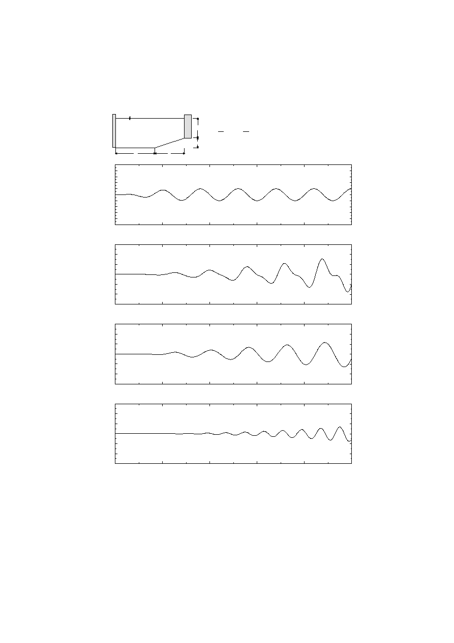
Following the procedure mentioned above some numerical computations have been

performed. The frequency of the generation was chosen to be equal to the resonance
frequency of the fluid domain (the length of the generated wave was equal twice the
distance ED in Fig.1.). Some of the results of computations are illustrated in Fig.2, where
the free surface elevation at the right boundary (the vertical displacement of the point D in
the figure) and the resultant of pressure forces acting on the boundary, and its moment
relative to point C in the figure, are depicted in the subsequent plots. Since we are dealing
with generation of resonance frequency, the calculated quantities grow in time. From the
plots it is seen that the linear component of the solution behaves like a linear oscillator in
the resonance range i.e. it grows in time according to the formula

t

t



sin

. The frequency

of the second component of the solution equals twice of the first component. The main
feature of the second component is that it grows in time in an exponential manner, and thus,
the solution obtained is valid only in a limited range of time. One should remember that in
constructing the approximate solution it has been assumed that the second component of the
solution should be sufficiently small as compared to the first order one. The results obtained
allow us to examine main features of the discrete formulation of the non-linear problem
considered.

9

0

50

100

150

200

250

Time step

-5

-4

-3

-2

-1

0

1

2

3

4

5

D

is

pl

ac

em

en

t

[c

m

]

0

50

100

150

200

250

Time step

-15

-10

-5

0

5

10

15

D

is

pl

ac

em

en

t

[c

m

]

0

50

100

150

200

250

Time step

-15

-10

-5

0

5

10

15

D

is

pl

ac

em

en

t

[c

m

]

0

50

100

150

200

250

Time step

-15

-10

-5

0

5

10

15

D

is

pl

ac

em

en

t

[c

m

]

A

B

C

D

E

a

b

d

c

Surface elevation at "D".

First order term.

Second order term.

Generator motion.

Fig. 2. Generation of standing waves in fluid domain with sloping bottom.

s

t

de

c

d

b

a

0541

.

0

1

5

1











,

,

,

10

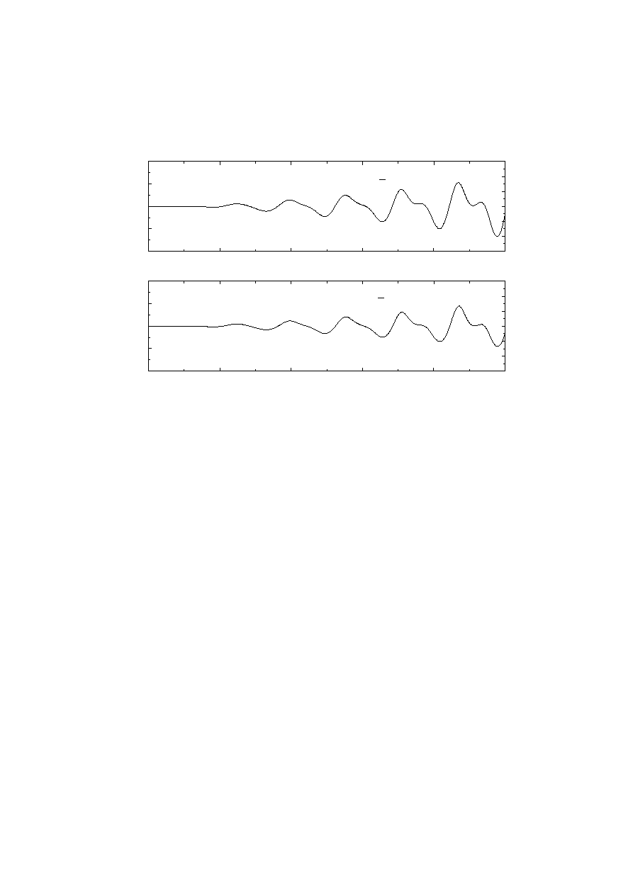
Fig. 2. Continued.

0

50

100

150

200

250

Time step

0.50

0.75

1.00

1.25

1.50

F

or

ce

0

50

100

150

200

250

Time step

0.0

0.5

1.0

1.5

2.0

M

om

en

t

Resultant of pressure on CD =





gd

2

x

f

Moment of pressure on CD =





gd

3

x

f

1

6

1

2

f

f

REFERENCES

1.

Bathe K. J. (1982) Finite Element Procedures in Engineering Analysis, Prentice-Hall,
Inc., Englewood Cliffs, New Jersey.

2.

Szmidt J.K. (2001) Zbadanie dyskretnego rozwiązania potencjalnego ruchu falowego
cieczy w zmiennych Lagrange’a, oprac. wewn. IBW-PAN, str. 1-31.

3.

Wehausen J. V. and Laitone E. V. (1960) Surface Waves in Encyclopaedia of Physics
ed. by Flugge S., vol. IX, Fluid Dynamics III, Springer Verlag, Berlin.

4.

Wilde P. and Wilde M. (2001) On the Generation of Water Waves in a Flume,
Archives of Hydro-Engineering and Environmental Mechanics, vol. 48, No.4, pp.69-
83.

Fale stojące o skończonej amplitudzie w wodzie

o zmiennej głębokości

STRESZCZENIE

W pracy dyskutuje się rozwiązanie dyskretne zagadnienia narastającej fali stojącej o
skończonej amplitudzie. W analizowanym modelu jest to wymuszenie ruchu cieczy w ob-
szarze skończonym za pomocą generatora typu sztywnego tłoka. Częstość wymuszenia od-
powiada częstości rezonansowej obszaru cieczy. Cały układ rozpoczyna ruch ze stanu spo-
koju. Rozwiązanie zbudowano za pomocą metody małego parametru, przy ograniczeniu
rozwiązania do drugiego rzędu przybliżenia. Rozważania zilustrowano przykładem licz-
bowym dotyczącym pionowego falochronu w wodzie o liniowo zmiennej głębokości.

11