14.1

Chapter Fourteen

One Dimension Again

14.1 Scalar Line Integrals

Now we again consider the idea of the integral in one dimension. When we were

introduced to the integral back in elementary school, we considered only functions defined

on nice subsets of the real line. The notion of an integral of a function f : D

R

→

in

which D is a nice one dimensional set, but is not a subset of the reals is our next object of

study. To get some idea of why one might care about such a thing, consider the simple

problem of finding the mass of a piece of wire having the shape of an arc of a space curve

C and having a given density

ρ

( )

r . How might we approach such a problem? Simple

enough! We subdivide, or partition, the curve with a finite set of points, say

{ , ,

, }

r r

r

0

1

K

n

. On the subarc joining r

i

−

1

to r

i

, we choose a point, say r

i

*

, and evaluate

the function

ρ

(

)

*

r

i

. Now we multiply this times the length of the line segment joining the

points r

i

−

1

and r

i

for an approximation to the mass of this arc of our curve. Then sum

these to obtain an approximation for the total mass:

S

i

i

i

i

n

=

−

−

=

∑

ρ

(

)|

|

*

r

r

r

1

1

.

Then we all believe that the "limit" of these sums as we choose finer and finer partitions

of the curve should be the actual, honest-to-goodness mass of the wire.

Let's abstract the essence of the discussion. Suppose f :C

R

→

is a function

whose domain C is a curve (in R

R

2

3

or

, or wherever). We subdivide the curve as in the

preceding discussion and choose a point r

i

*

on the subarc joining r

i

−

1

to r

i

. The sum

14.2

S

f

i

i

i

i

n

=

−

−

=

∑

(

)|

|

*

r

r

r

1

1

again is called a Riemann sum. If there is a number L such that all Riemann sums are

arbitrarily close to L for sufficiently fine partitions, then we say f is integrable on C, and

the number L is called the integral of f on C and is denoted

f

d

( )

r r

C

∫

. This integral is

also frequently referred to as a line integral.

This is wonderful, but how do find such an integral? It is remarkably simple and

easy. Suppose we have a vector description of the curve C; say r( )

t

a

t

b

, for

≤ ≤

. We

partition the curve by partitioning the interval [ , ]

a b : If {

, ,

,

}

a

t t

t

b

n

=

=

0

1

K

is a partition

of the interval, then the points { ( ), ( ),

, ( )}

r

r

r

t

t

t

n

0

1

K

partition the curve C. We obtain

the point r

i

*

on the subarc joining r(

)

t

i

−

1

to r( )

t

i

by choosing t

t

t

i

i

i

*

[

, ]

∈

−

1

and letting

r

r

i

i

t

*

*

( )

=

. Our Riemann sum now looks like

S

f

t

t

t

i

i

i

i

n

=

−

−

=

∑

( ( )| ( )

(

)|

*

r

r

r

1

1

.

14.3

Next, multiply the terms on the right by one, but one disguised as

∆
∆

t

t

i

i

, where, of course,

∆

t

t

t

i

i

i

= −

−

1

. Then we see

S

f

t

t

t

t

t

i

i

i

i

i

n

i

=

−

−

=

∑

( ( )

( )

(

)

*

r

r

r

1

1

∆

∆

.

We know that lim

( )

(

)

∆

∆

t

i

i

i

t

t

t

d

dt

→

−

−

=

0

1

r

r

r

, and so it is not hard to convince oneself that the

"limiting" value of the Riemann sums is

f

t

d t

dt

dt

a

b

( ( ))

( )

r

r

∫

.

We have thus turned the problem into one we know how to solve—a plain old everyday

elementary calculus integral. Hence,

f

d

f

t

d t

dt

dt

a

b

( )

( ( ))

( )

r r

r

r

C

∫

∫

=

.

Example

Suppose we have a wire in the shape of a quarter circle of radius 2, and the

density of the wire is given by

ρ

( , )

x y

y

=

. What is the mass of the wire? Well, we

know the mass is simply the integral ydr

C

∫

, where C is the quarter circle:

14.4

A vector description of the curve is r

i

j

( )

cos

sin

t

t

t

=

+

2

2

, for 0

4

≤ ≤

t

π

. Thus we have

d

dt

t

t

r

i

j

=−

+

=

|

sin

cos |

2

2

2 , and the integral becomes simply

yd

t dt

r

C

∫

∫

=

=

4

4

0

4

sin

/

π

.

Let's see what happens if we use a different vector description of the curve, say

r

i

j

( )

t

t

t

= +

−

4

2

for 0

2

≤ ≤

t

. We have

d

dt

t

t

t

r

i

j

= −

−

=

−

4

2

4

2

2

. Hence

yd

t

t

dt

dt

r

C

∫

∫

∫

=

−

−









 =

=

4

2

4

2

4

2

2

0

2

0

2

.

We get, as we must, the same answer.

Exercises

1. Evaluate the integral (

)

x

y

z

d

− + +

∫

2

r

C

, where C is the curve r

i

j

k

( )

(

)

t

t

t

= + −

+

1

,

0

1

≤ ≤

t

.

14.5

2. Evaluate the integral

x

y d

2

2

+

∫

r

C

, where C is the curve r

i

j

k

( )

cos

sin

t

t

t

t

=

+

+

4

4

3

,

−

≤ ≤

2

2

π

π

t

.

3. Find the centroid of a semicircle of radius a.

4. Find the mass of a wire having the shape of the curve r

j

k

( )

(

)

t

t

t

t

=

−

+

≤ ≤

2

1

2

0

1

,

if the density is

ρ

( )

t

t

=

3

2

.

5. Find the center of mass of a wire having the shape of the curve

r

i

j

k

( )

/

t

t

t

t

t

= +

+

≤ ≤

2 2

3

2

0

2

3 2

2

,

,

if the density is

ρ

( )

t

t

=

+

1

1

.

6. What is dr

C

∫

?

14.2 Vector Line Integrals

Now we are introduce something perhaps a little different from what we have seen

to now—integrals with vector valued integrands. Specifically, suppose C is a space curve

and f C

R

3

:

→

is a function from C into the Euclidean space R

3

. We are going to define

an integral

f r

r

C

( )

⋅

∫

d . Why should we care about such a thing? Again, let's think about a

physical model. You learned in fifth grade physics that the work done by a force F acting

through a distance d is simply the product Fd. The force F and the displacement d are, of

course, really vectors, and we saw earlier in life that the "product" of the two is actually

14.6

the scalar, or dot, product of the two vectors. Now, in general, neither of these quantities

will be constant, and we will have a variable force F(r) acting along a curve C in space.

How do we compute the work done in this situation? Let's see. Once more, we partition

the curve by choosing a sequence of points { , ,

, }

r r

r

0

1

K

n

on the curve, with r

0

being the

initial point and r

n

being the final point. Now, of course, there is an orientation, or

direction, specified on the curve. One may think of specifying an orientation by simply

putting an arrow on the curve—it thus makes sense to speak of the initial point and the

terminal point of the curve. Exactly as in the scalar integrand case, we choose a point r

i

*

on the subarc joining r

i

−

1

to r

i

, and evaluate F r

(

)

*

i

. Now then, the work done in going

from r

i

−

1

to r

i

is approximately the scalar product F r

r

r

(

) (

)

*

i

i

i

⋅

−

−

1

. Add all these up for

an approximation to the total work done:

S

i

i

i

i

n

=

⋅

−

−

=

∑

F r

r

r

(

) (

)

*

1

1

.

The course should be obvious now; we take finer and finer partitions, and the limiting

value of the sums is the integral

F r

r

C

( )

⋅

∫

d .

This integral too is called a line integral. To prevent confusion, we sometimes

speak of scalar line integrals and vector line integrals. How to find such a vector integral

should be clear from the discussion of scalar line integrals. We let r( ),

t

a

t

b

≤ ≤

, be a

vector description of C. (Here r( )

a is the initial point and r( )

b is the terminal point.)

The discussion proceeds almost exactly as it did in the previous section and we get

14.7

F r

r

F r

r

C

( )

( ( ))

⋅ =

⋅

∫

∫

d

t

d

dt

dt

a

b

.

Example

Find [(

)

(

)

]

xy

z

x

z

yz

d

+

+

+

+

⋅

∫

2

2

i

j

k

r

C

, where C is the straight line from the

origin to the point (1,2,3). The line C has a vector description r

i

j

k

( )

t

t

t

t

= +

+

2

3

. Thus,

d

dt

r

i

j

k

= +

+

2

3 , and so

[(

)

(

)

]

[(

)

(

)

] (

)

(

)

(

)

xy

z

x

z

yz

d

t

t

t

t

t

dt

t

t

t dt

t

t dt

+

+ +

+

⋅

=

+

+ +

+

⋅ +

+

=

+ +

=

+

∫

∫

∫

∫

2

2

2

2

0

1

2

2

0

1

2

0

1

2

2

9

3

12

2

3

2

8

36

38

8

i

j

k

r

i

j

k

i

j

k

C

=

+

=

38

3

4

50

3

3

2

0

1

t

t

.

Nothing to it.

Another Example

Now let's integrate the same function from (0,0,0) t0 (1,2,3), but this time along

the path P in the picture:

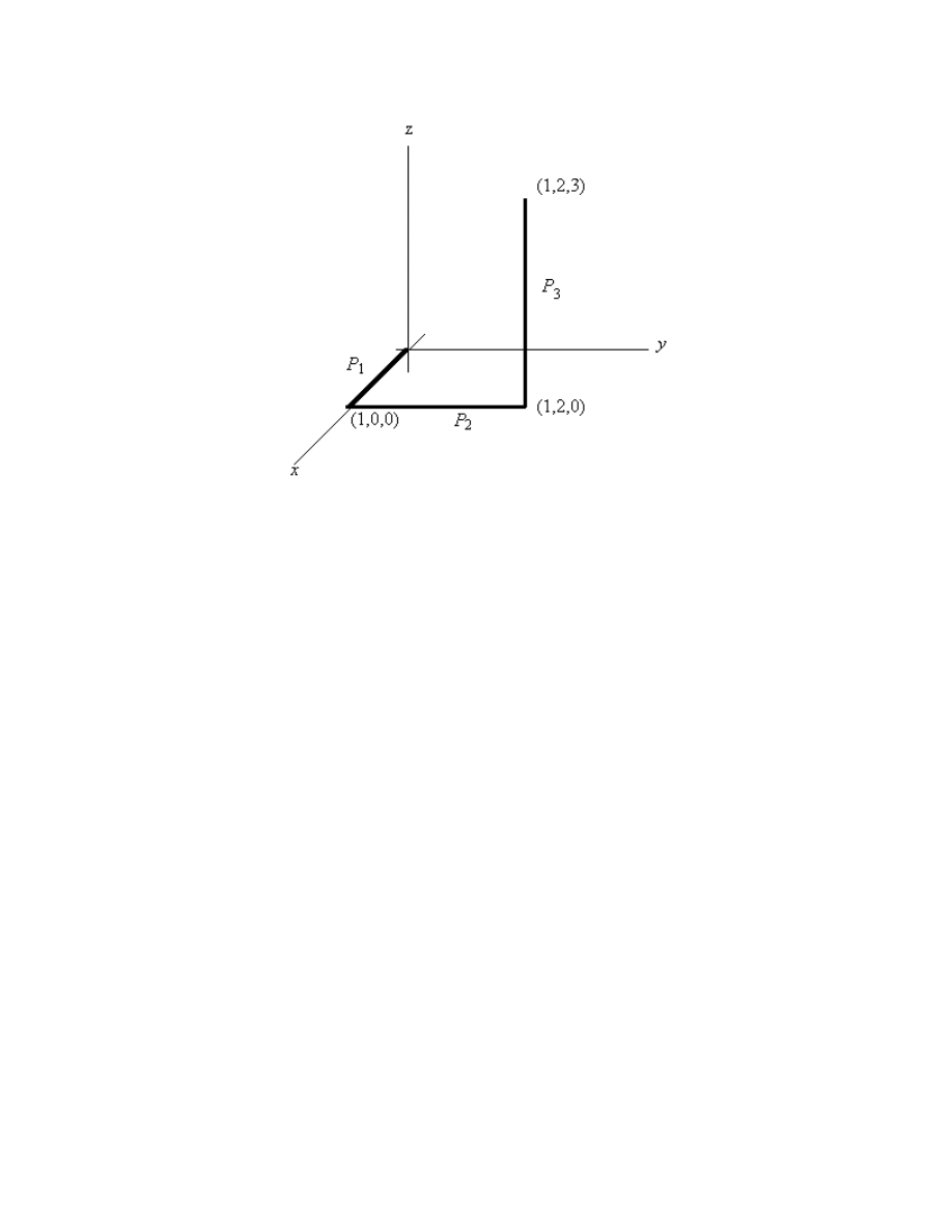
14.8

Here the path P is the union of the three nice curves, P P

1

2

,

, and

P

3

, so our integral is the

sum of three integrals:

F

r

F

r

F

r

F

r

( , , )

( , , )

( , , )

( , , )

x y x d

x y x

d

x y x

d

x y x

d

P

P

P

P

⋅ =

⋅ +

⋅ +

⋅

∫

∫

∫

∫

3

2

1

,

where

F

i

j

k

( , , )

(

)

(

)

x y z

xy

z

x

z

yz

=

+

+ +

+

2

2

.

A vector description of P

1

is simply r

i

( )

t

t

t

=

≤ ≤

, 0

1. Thus

F

r

F

i

j i

( , , )

( , , )

x y z

d

t

dt

t

dt

P

⋅

=

⋅

=

⋅

=

∫

∫

∫

00

0

0

1

0

1

1

.

For

P

2

, we have r

i

j

( )

,

t

t

= +

≤ ≤

0

t

2 . This gives us

F

r

F

j

i

j

j

( , , )

( , , )

(

)

x y z

d

t

dt

t

dt

dt

P

⋅

=

⋅

=

+ ⋅

=

=

∫

∫

∫

∫

1

0

2

0

2

0

2

0

2

2

.

14.9

Finally, for

P

3

, there is r

i

j

k

( )

t

t

t

= +

+

≤ ≤

2

0

3

,

; and so

F

r

F

k

i

j

k

k

( , , )

( , , )

[(

)

(

)

]

x y z

d

t

dt

t

t

t

dt

P

⋅

=

⋅

=

+

+ +

+

⋅

∫

∫

∫

3

12

2

1

4

2

0

3

0

3

=

=

∫

4

18

0

3

t dt

.

At last, we have then F

r

( , , )

x y z d

P

⋅ = + +

=

∫

0

2

18

20 .

Exercises

7. Evaluate [

]

xy

x

d

C

i

j

r

+

⋅

∫

2

, where C is the arc of the curve y

x

=

2

from (0,0) to (1,1).

8. Evaluate (cos

)

x

y

d

C

i

j

r

−

⋅

∫

where C the part of the curve y

x

=

sin from (0,0) to

(

π

,0).

9. Evaluate the line integral of F

i

j

k

( , , )

(

)

x y z

xyz

xy

yz

z

=

+

+

+

2

from (0,0,0) to

(-1,1,2) along the line segment joining these two points.

10. Evaluate the line integral of F

i

j

k

( , , )

(

)

(

)

(

)

x y z

x

z

y

z

x

y

=

−

+

−

− +

along the

polygonal path from (0,0,0) to (1,0,0) to (1,1,0) to (1,1,1).

11. Integrate F

i

j

( , )

(

)

x y

x

y

y

x

=

+

− +

1

2

2

one time around the circle x

y

a

2

2

2

+

=

in the

counterclockwise direction.

14.10

14.3 Path Independence

Suppose we evaluate the vector line integral F r

r

( )

⋅

∫

d

C

, where C is a curve from

the point p to the point q. Let r( ),

t

a

t

b

≤ ≤

, be a vector description of C. Then, of

course, we have r

p

( )

a

=

and r

q

( )

b

=

. As we have already seen,

F r

r

F r

r

( )

( ( ))

⋅ =

⋅

∫

∫

d

t

d

dt

dt

a

b

C

.

Now let us make the very special assumption that there exists a real-valued (or scalar)

function g: R

R

3

→

such that the derivative, or gradient, of g is the integrand F :

∇ =

g

F .

Next let's use the Chain Rule to compute the derivative of the composition

h t

g

t

( )

( ( ))

=

r

:

h t

g

d

dt

t

d

dt

'( )

( ( ))

= ∇ ⋅

=

⋅

r

F r

r

.

This is, mirabile dictu, precisely the integrand in our line integral:

F r

r

F r

r

p

q

( )

( ( ))

'( )

( )

( )

( )

( )

⋅

=

⋅

=

=

−

=

−

∫

∫

∫

d

t

d

dt

dt

h t dt

h b

h a

g

g

a

b

C

a

b

.

This is a very exciting result and calls for some meditation. Note that the curve C

has completely disappeared from the answer. The value of the integral depends only on

the values of the function g at the endpoints; the path from p to q does not affect the

answer. The line integral is path independent. The result is esthetically pleasing and is

clearly the lineal descendant of the fundamental theorem of calculus we learned so many

years ago.

14.11

A moment's reflection on the examples we have seen should convince us that a lot

of integrals are not path independent, thus many very nice functions F (or vector fields )

are not the gradient of any function. A function F that is the gradient of a function g is

said to be conservative and the function g is said to be a potential function for F.

Let's suppose the domain D of the function F D

R

3

:

→

is open and connected

(Thus any two points in D may be joined by a nice path.) We have just seen that if there

exists a function g: D

R

→

such that F

= ∇

g , then the integral of F between any two

points of D does not depend on the path between the two points. It turns out, as we

shall see, that the converse of this is true. Specifically, if every integral of F in D is path

independent, then there is a function g such that F

= ∇

g . Let's see why this is so.

Choose a point p

D

=

∈

(

,

,

)

x y z

0

0

0

. Now define g

g x y z

( )

( , , )

s

=

to be the

integral from p to s along any curve joining these points. We are assuming path

independence of the integral, so it matters not what curve we choose. Okay, now we

compute the partial derivative

∂

∂

g

x

. The domain D is open and hence includes an open

ball centered at s

D

=

∈

( , , )

x y z

. Choose a point q

=

(

, , )

x y z

1

in such an open ball, and

let L be the straight line segment from s to q . Then, of course, L lies in D. Now let's

integrate F from p to s by going along any curve C from p to q and then along L from q to

s :

g

g x y z

d

d

( )

( , , )

( )

( )

s

F r

r

F r

r

C

L

=

=

⋅ +

⋅

∫

∫

.

The first integral on the right does not depend on x, and so

∂

∂

x

d

F r

r

C

( )

⋅ =

∫

0 . Thus

∂

∂

∂

∂

g

x

x

d

=

⋅

∫

F r

r

L

( )

.

14.12

We clearly need to find F r

r

L

( )

⋅

∫

d . This is easy. Suppose

F r

r i

r j

r k

( )

( )

( )

( )

=

+

+

f

f

f

1

2

3

.

A vector description of L is simply r

i

j

k

( )

,

t

t

y

z

x

t

x

= + +

≤ ≤

1

. Thus

d

dt

r

i

=

, and our

line integral becomes simply F r

r

L

( )

( , , )

⋅

=

∫

∫

d

f t y z dt

x

x

1

1

. We are almost done, for note

that now

∂

∂

∂

∂

x

d

x

f t y z dt

f x y z

x

x

F r

r

L

( )

( , , )

( , , )

⋅ =

=

∫

∫

1

1

1

.

Hence

∂

∂

g

x

f

=

1

.

It should be clear to one and all how to show that

∂

∂

g

y

f

=

2

and

∂

∂

g

z

f

=

3

, thus

giving us the desired result: F

= ∇

g .

Exercises

12. Prove that

∂

∂

g

y

f

=

2

, where g and

f

2

are as in the preceding discussion.

13. Prove that if F D

R

3

:

→

, where D is open and connected, and every

F r

r

C

( )

⋅

∫

d is

path independent, then F r

r

P

( )

⋅

=

∫

d

0 for every closed path in D.( A closed path, or

14.13

curve, is one with no endpoints.) [Physicists and others like to use a snake sign with a

little circle superimposed on it

∫

to indicate that the path of integration is closed.]

14. Prove that if F D

R

3

:

→

, where D is open and connected, and

F r

r

P

( )

⋅

=

∫

d

0 for

every closed path in D, then every F r

r

C

( )

⋅

∫

d is path independent .

15. a)Find a potential function g for the function F r

i

j

k

( )

=

+

+

yz

xz

xy .

b)Evaluate the line integral F r

r

C

( )

⋅

∫

d , where C is the curve

r

i

j

k

( )

(

sin )

cos

,

t

e

t

t e

t

t

t

t

=

+

+

≤ ≤

2

3

3

0

1

.

16. a)Find a potential function g for the function F r

i

j

k

( )

(

)

=

+ +

+

e

x

x

y

z

2

2

.

b)Find another potential function for F in part a).

b)Evaluate the line integral F r

r

C

( )

⋅

∫

d , where C is the curve

r

i

j

k

( )

cos

t

t

t

t

e

t

t

=

+

+

≤ ≤

2

4

0

2

2

,

π

.

17. Evaluate

[(

sin

)

(

cos

) ]

e

y

y

e

y

x

y

d

x

x

+

+

+

−

⋅

∫

3

2

2

i

j

r

E

where E is the ellipse

4

4

2

2

x

y

+

=

oriented clockwise.

[Really good hint: Find the gradient of g x y z

e

y

xy

y

x

( , , )

sin

=

+

−

2

2

.]