12.1

Chapter Twelve

Integration

12.1 Introduction

We now turn our attention to the idea of an integral in dimensions higher than one.

Consider a real-valued function f : D

R

→

, where the domain D is a nice closed subset of

Euclidean n-space R

n

. We shall begin by seeing what we mean by the integral of f over

the set D; then later we shall see just what such an abstract thing might be good for in real

life. Mrs. Turner taught us all about the case

n

=

1

. As it was in extending the definition

of a derivative to higher dimensions, our definition of the integral in higher dimensions will

include the definition for dimension 1 we learned in grammar school—as always, there

will be nothing to unlearn. Let us again hark back to our youth and review what we know

about the integral of f : D

R

→

in case D is a nice connected piece of the real line R.

First, in this context, the only nice closed pieces of R are the closed intervals; we thus

have D is a set [ , ]

a b , where b

a

>

. Recall that we defined a partition P of the interval to

be simply a finite subset {

,

,

,

}

x x

x

n

0

1

K

of [ , ]

a b with a

x

x

x

x

b

n

=

<

<

< <

=

0

1

2

K

.

The mesh of a partition is max{|

|:

,

, }

x

x

i

n

i

i

−

=

−

1

12

K

. We then defined a Riemann sum

S P

( ) for this partition to be a sum

S P

f x

x

i

i

i

n

( )

(

)

*

=

=

∑

∆

1

,

where

∆

x

x

x

i

i

i

= −

−

1

is simply the length of the subinterval [

,

]

x

x

i

i

−

1

and

x

i

*

is any point

in this subinterval. (Thus there is not just one Riemann sum for a partition P; the sum

obviously also depends on the choices of the points

x

i

*

. This is not reflected in the

notation.)

Now, if there is a number L such that we can make all Riemann sums as close as we

like to L by choosing the mesh of the partition sufficiently small, then f is said to be

12.2

integrable over the interval, and the number L is called the integral of f over [a, b]. This

number L is almost always denoted

f x dx

a

b

( )

∫

. More formally, we say that L is the

integral of f over [ , ]

a b if for every

ε >

0 , there is a

δ

so that | ( )

|

S P

L

− < ε

for every

partition P having mesh <

δ

. You no doubt remember from your first encounter with this

integral that it initially seemed like an impossible thing to compute in any reasonable

situation, but then some version of the Fundamental Theorem of Calculus came to the

rescue.

12.2 Two Dimensions

Let us begin our study of higher dimensional integrals with the two dimensional

case. As we have seen so often in the past, in extending calculus ideas to higher

dimensions, most of the excitement occurs in taking the step from one dimension to two

dimensions—seldom is the step from 97 to 98 dimensions very interesting. We shall thus

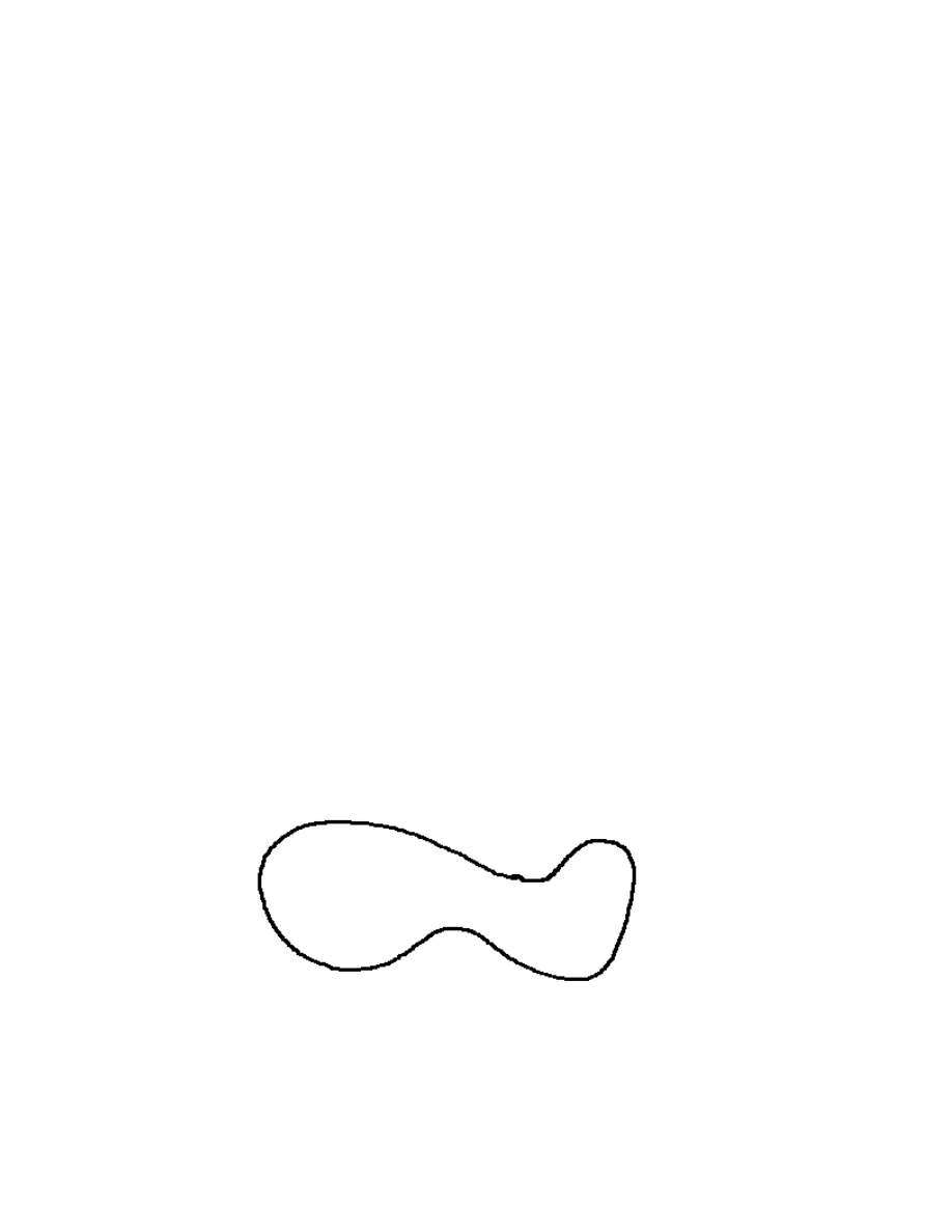
begin by looking at the integral of f : D

R

→

for the case in which D is a nice closed

subset of the plane. Complications appear at once. On the real line, nice closed sets are

simply closed intervals; in the plane, nice closed sets are considerably more interesting:

12.3

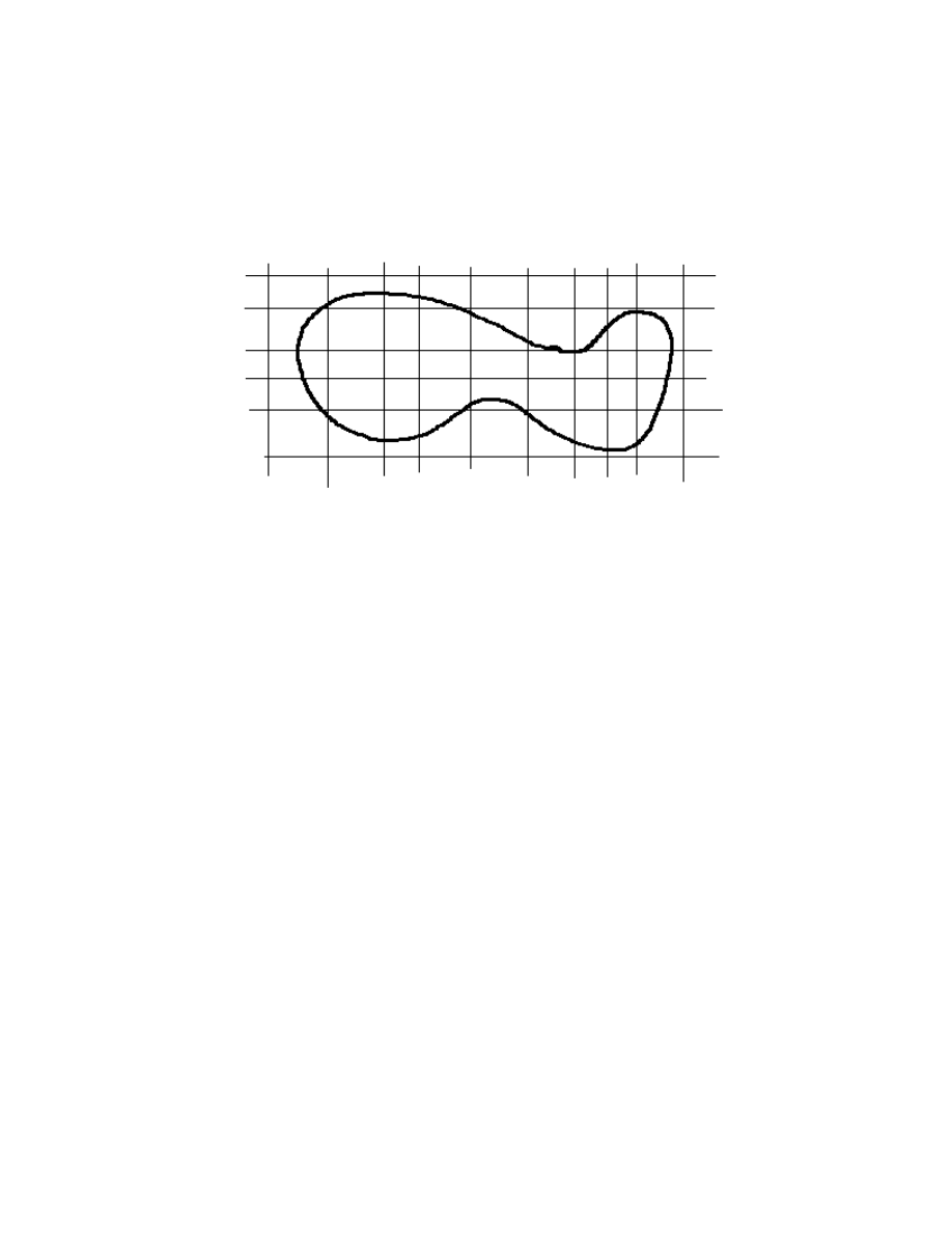
A moment's reflection convinces us that the domain D can, even in just two dimensions,

be considerably more complicated than it is in one dimension. First, capture D inside a

rectangle with sides parallel to the coordinate axes; and then divide this rectangle into

subrectangles by partitioning each of its sides:

Now, label the subrectangles that meet D, say with subscripts

i

n

=

12

, ,

,

K

. The largest

area of all such rectangles is called the mesh of the subdivision. In each such rectangle,

choose a point (

,

)

*

*

x y

i

i

in D. A Riemann sum S now looks like

S

f x

y

A

i

i

i

i

n

=

=

∑

(

,

)

*

*

∆

1

,

where

∆

A

i

is the area of the rectangle from which (

,

)

*

*

x y

i

i

is chosen. Now if there is a

number L such that we can get as close to L as we like by choosing the mesh of the

subdivision sufficiently small, then f is said to be integrable over D, and the number L is

the integral of f over D. The number L is usually written with two snake signs:

f x y dA

( , )

D

∫∫

.

Such integrals over two dimensional domains are frequently referred to as double

integrals.

12.4

I hope the definition of the integral in case D is a nice subset of R

3

is evident. We

capture D inside a box, and subdivide the box into boxes, etc. , etc. There will be more of

the higher dimensional stuff later.

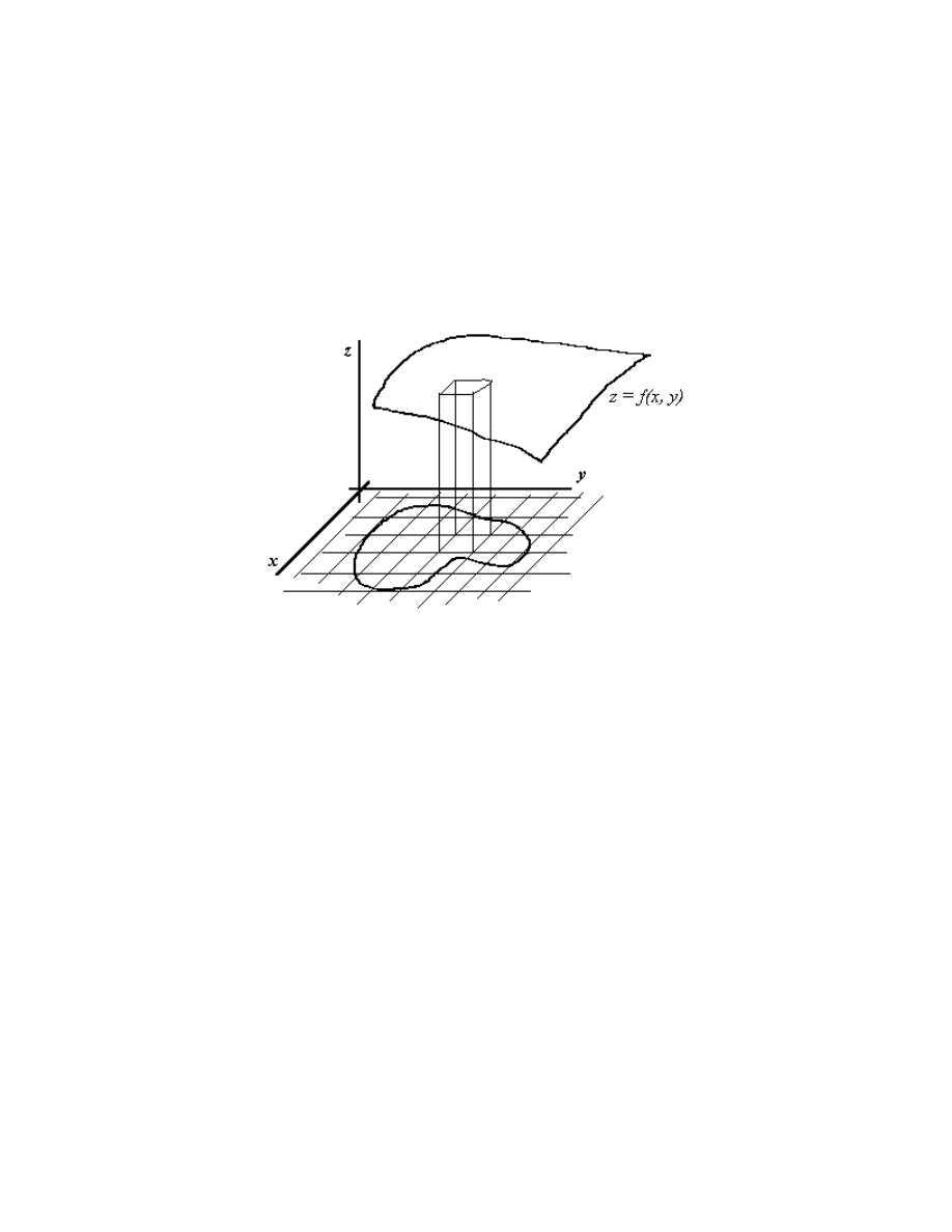
Let's look a bit at some geometry. For the purpose of drawing a reasonable picture,

let us suppose that f x y

( , )

≥

0 everywhere on D.

Each term f x y

A

i

i

i

(

,

)

*

*

∆

is the volume of a box with base the rectangle

A

i

and height

f x y

i

i

(

,

)

*

*

. The top of the box thus meets the surface z

f x y

=

( , ) . The Riemann sum is

thus the total volume of all such boxes. Convince yourself that as the size of the bases of

the boxes goes to 0, the boxes "fill up" the solid bounded below by the x-y plane, above

by the surface z

f x y

=

( , ) , and on the sides by the cylinder determined by the region D.

The integral

f x y dA

( , )

D

∫∫

is thus equal to the volume of this solid. If f x y

( , )

≤

0 , then,

of course, we get the negative of the volume bounded below by the surface z

f x y

=

( , ) ,

above by the x-y plane, etc.

Suppose a and b are constants, and D

E

F

= ∪

, where E and F are nice domains

whose interiors do not meet. The following important properties of the double integral

should be evident:

12.5

[

( , )

( , )]

( , )

( , )

af x y

bg x y dA

a

f x y dA b

g x y dA

+

=

+

∫∫

∫∫

∫∫

D

D

D

, and

f x y dA

f x y dA

f x y dA

( , )

( , )

( , )

D

E

F

∫∫

∫∫

∫∫

=

+

.

Now, how on Earth do we ever find an integral

f x y dA

( , )

D

∫∫

? Let's see. Again, we

shall look at a picture, and again we shall draw our picture as if f x y

( , )

≥

0 . It should be

clear what happens if this is not the case.

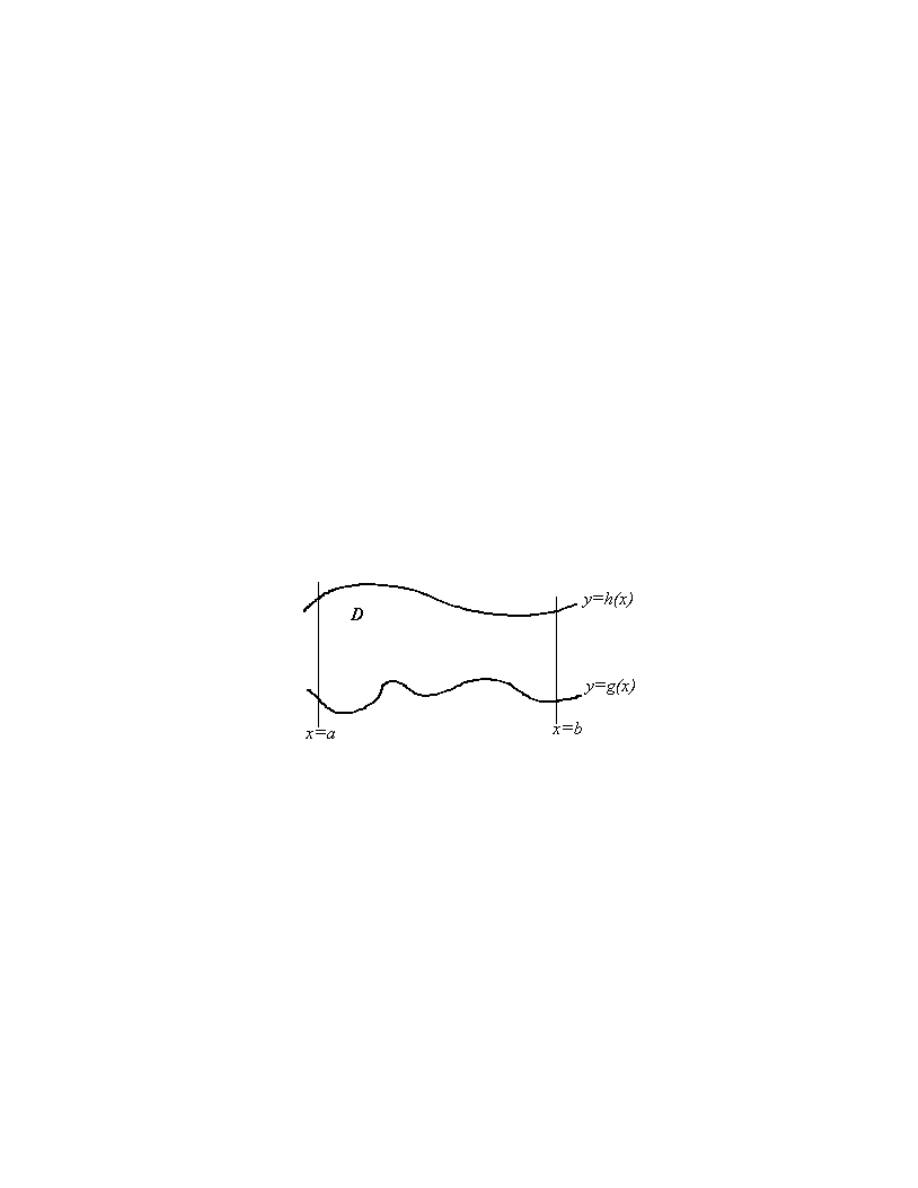
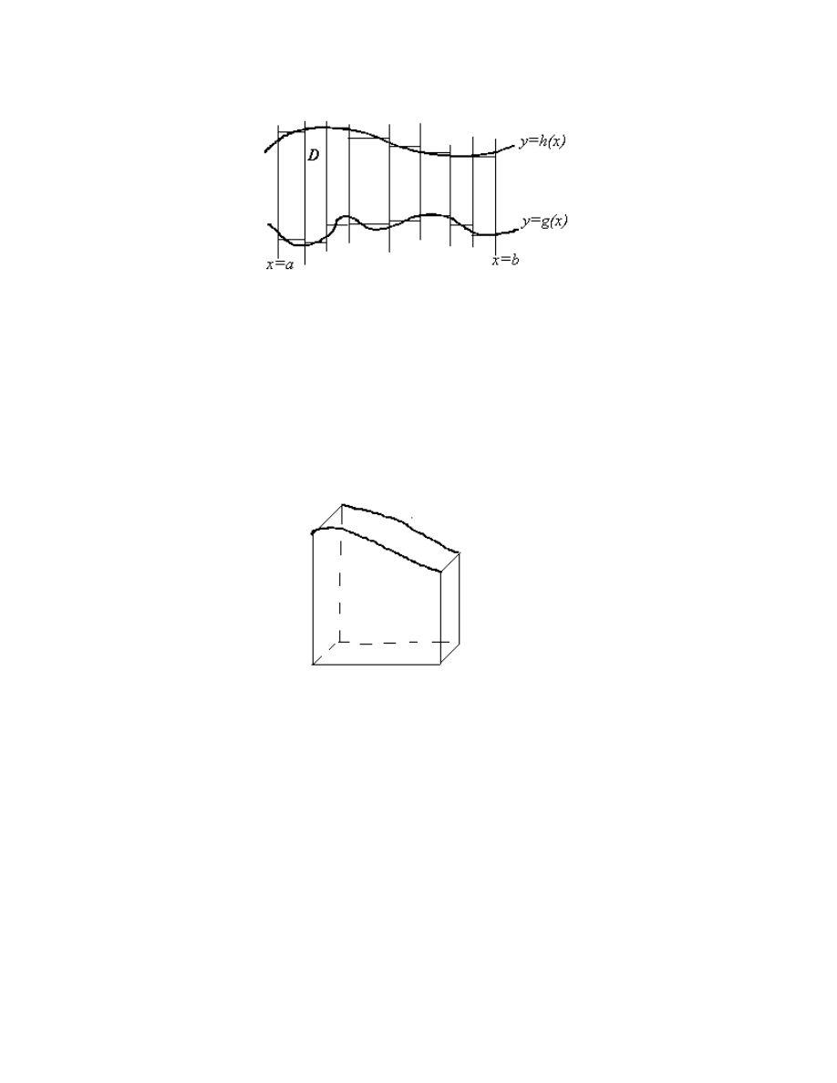
We assume our domain D has a special form; specifically, we suppose it to be

bounded above by the curve y

h x

=

( ) , below by y

g x

=

( ) , on the left by x

a

=

, and on

the right by x

b

=

:

It is convenient for us to think of the integral

f x y dA

( , )

D

∫∫

as the volume of the blob

bounded below by D in the x-y plane and above by the surface z

f x y

=

( , ) . Think of

finding this volume by dividing the blob into slices parallel to the y-axis and adding up the

volumes of the slices. To approximate the volumes of these slices, we use slabs:

12.6

We partition the x interval [a, b ]: a

x

x

x

x

b

n

n

=

<

< <

<

=

−

0

1

1

K

. In each subinterval

[

,

]

x

x

i

i

−

1

choose a point

x

i

*

. Our approximating slab has as its base the rectangle of

"width"

∆

x

x

x

i

i

i

= −

−

1

and height h x

g x

i

i

(

)

(

)

*

*

−

; the roof is z

f x y

i

=

(

, )

*

. The volume

of the slab is the cross section area times the thickness, or [

(

, )

]

*

(

)

(

)

*

*

f x

y dy

x

i

g x

h x

i

i

i

∫

∆

.

The sum of the volumes of the approximating slabs is thus

S

f x

y dy

x

i

g x

h x

i

i

n

i

i

=

∫

∑

=

[

(

, )

]

*

(

)

(

)

*

*

∆

1

.

The double integral we seek is just the "limit" of these as we take thinner and thinner

slabs; or finer and finer partitions of the interval [a, b]. But Lo! The above sums are

12.7

Riemann sums for the ordinary one dimensional integral of the function

F x

f x y dy

g x

h x

( )

( , )

( )

( )

=

∫

, and so the double integral is given by

f x y dA

F x dx

f x y dy dx

a

b

g x

h x

a

b

( , )

( )

[

( , )

]

( )

( )

=

=

∫

∫∫

∫

∫

D

The double integral is thus equal to an integral of an integral, usually called an iterated

integral. It is traditional to omit the brackets and write the iterated integral simply as

f x y dydx

g x

h x

a

b

( , )

( )

( )

∫

∫

.

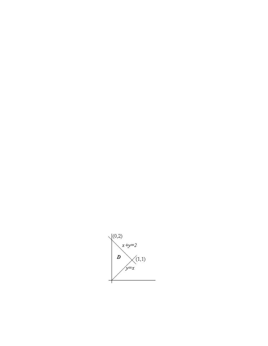
Example

Let's find the double integral

[

]

x

y dA

2

2

+

∫∫

D

, where D is the area enclosed by the

lines y

x

=

, x

=

0 , and x

y

+ =

2 . The first item of business here is to draw a picture of

D (We always need a picture of the domain of integration.):

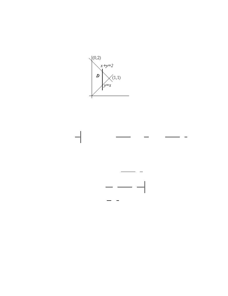
12.8

It should be clear from the picture that in the language of our discussion, g x

x

( )

=

,

h x

x

( )

= −

2

, a

=

0 , and b

=

1. So slice parallel to the y axis:

The lower end of the slice is at y

x

=

and the upper end is at y

x

= −

2

. The "volume" is

thus

[

]

(

)

(

)

(

)

x

y dy

x y

y

x

x

x

x

x

x

x

x

x

x

y x

y

x

2

2

2

2

3

2

2

3

3

3

2

3

3

3

2

2

3

3

2

2

3

7

3

+

=

+

=

− +

−

−

−

=

+

−

−

−

=

= −

∫

,

and we have such a slice for all x from x

=

0 to x

=

1. Thus

[

]

[

(

)

]

(

)

x

y dA

x

x

x dx

x

x

x

2

2

2

3

3

0

1

3

4

4

0

1

2

2

3

7

3

2

3

2

12

7

12

16

12

4

3

+

=

+

−

−

=

−

−

−

=

=

∫

∫∫

D

Exercises

1. Find

x dA

2

D

∫∫

, where D is the domain bounded by the curves y

x

= −

4

2

and y

x

=

3 .

12.9

2. Find

(

)

x

y dA

2

−

∫∫

D

, where D is the area in the first quadrant enclosed by the

coordinate axes and the line 2

4

x

y

+ =

.

3. Use double integration to find the area of the region enclosed by the curves x

y

− =

2

and y

x

= −

2

.

4. Find the volume of the solid cut from the first octant by the surface z

x

y

= −

−

4

2

.

5. Sketch the domain of integration and evaluate the iterated integral:

y e dydx

xy

x

2

1

0

1

∫

∫

.

6. Sketch the domain of integration and evaluate the iterated integral:

e

dydx

x y

x

+

∫

∫

0

1

8 l o g

log

.

7. Find the volume of the wedge cut from the first octant by the cylinder z

=

12

−

3y

2

and the plane x

y

+ =

2 .

8. Suppose you have a double integral

f x y dA

( , )

D

∫∫

in which the domain D is bounded

on the left by the curve x

g y

=

( ) , on the right by x

h y

=

( ) , below by y

a

=

, and

above by y

b

=

.

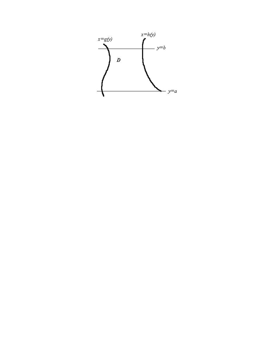
12.10

Give an iterated integral for the double integral in which the first integration is with

respect to x , and explain what's going on.

9. Give a double integral for the area of the region bounded by x

y

=

2

and x

y

y

=

−

2

2

,

and evaluate the integral.