13.1

Chapter Thirteen

More Integration

13.1 Some Applications

Think now for a moment back to elementary school physics. Suppose we have a

system of point masses and forces acting on the masses. Specifically, suppose that for

each

i

n

=

12

, ,

,

K

we have a point mass

m

i

whose position in space at time t is given by

the vector r

i

.. Assume moreover that there is a force f

i

acting on this mass. Thus

according to Sir Isaac Newton, we have

f

r

i

i

i

m

d

dt

=

2

2

for each i. Now sum these equations to get

F

f

r

=

=

=

=

∑

∑

i

i

n

i

i

i

n

m

d

dt

1

2

2

1

, or

F

r

=

























=

=

∑

∑

M

d

dt

m

m

i i

i

n

i

i

n

2

1

1

,

where M

m

i

i

n

=

=

∑

1

. Reflect for a moment on this equation. If we define R by

R

r

=

=

=

∑

∑

m

m

i i

i

n

i

i

n

1

1

, then the equation becomes F

R

=

M

d

dt

2

2

. Thus the sum of the external

forces on the system of masses is the total mass times the acceleration of the mystical

point R. This point R is called the center of mass of the system.

In case the total mass is continuously distributed in space, the "sum" in the

equation for R becomes an integral. Let's look at what this means in two dimensions.

13.2

Suppose we have a plate and the mass density of the plate at (x,y) is given by

ρ

( , )

x y .

To find the center of mass of the plate, we approximate its location by chopping it into a

bunch of small pieces and treating each of these pieces as a point mass.

Now choose a point r

i

j

i

i

i

x

y

=

+

*

*

in each rectangle. The mass of this rectangle will be

approximately

ρ

(

,

)

*

*

x

y

A

i

i

i

∆

, where

∆

A

i

is the area of the rectangle. The equation for the

center of mass of this system of rectangles is then

~

(

,

)

(

,

)

(

,

)

(

,

)

(

,

)

*

*

*

*

*

*

*

*

*

*

*

*

R

r

r

i

j

=

=

=









 +























=

=

=

=

=

=

=

∑

∑

∑

∑

∑

∑

∑

m

m

x

y

A

x y

A

x y

A

x

y x

A

x y

y

A

i i

i

n

i

i

n

i

i

i

i

i

n

i

i

i

i

n

i

i

i

i

n

i

i

i

i

i

n

i

i

i

i

i

n

1

1

1

1

1

1

1

1

ρ

ρ

ρ

ρ

ρ

∆

∆

∆

∆

∆

The three sums in the previous line are Riemann sums for two dimensional integrals!

Thus as we take smaller and smaller rectangles, etc., we obtain for R, the location of the

center of mass

13.3

R

i

j

=









 +

























∫∫

∫∫

∫∫

1

ρ

ρ

ρ

( , )

( , )

( , )

x y dA

x

x y dA

y

x y dA

P

P

P

In other words, the coordinates ( , )

x y of the center of mass of P are given by

x

x

x y dA

M

y

y

x y dA

M

P

P

=











=











∫∫

∫∫

ρ

ρ

( , )

( , )

, and

,

where M

x y dA

P

=

∫∫

ρ

( , )

is the total mass of the plate.

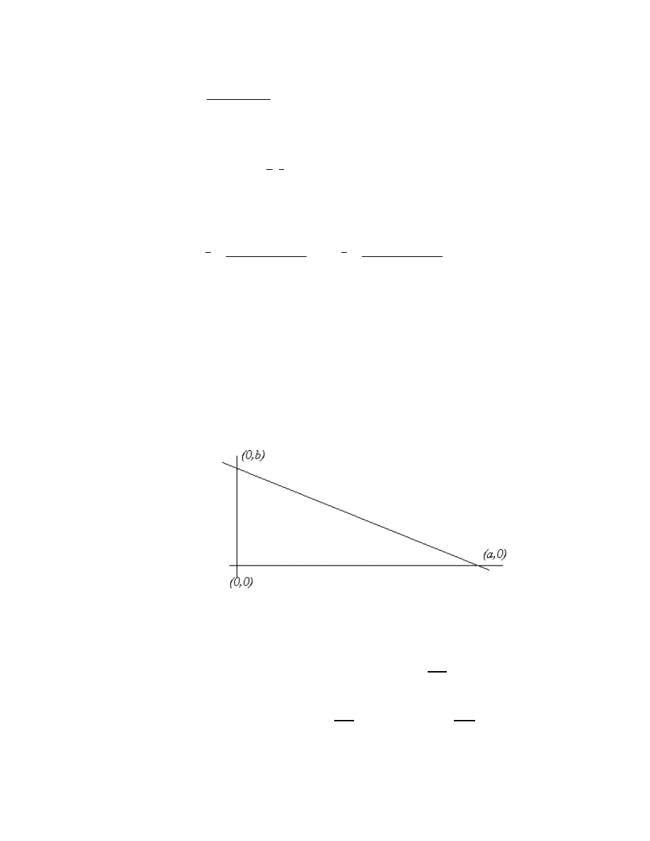
Example

Let's find the center of mass of a plate having the shape of the plane region

enclosed by the triangle

and having constant density (In this case, we say the mass is uniformly distributed over

the region. Suppose

ρ

( , )

x y

k

=

. First,

x

x y dA

k

xdydx

k xb

x a dx

k

a b

b

x a

a

T

a

ρ

( , )

(

/ )

(

/ )

=

=

−

=

−

∫

∫

∫∫

∫

0

1

0

2

0

1

6

, and then

y

x y dA

k

ydydx

kb

x a

dx

k

ab

b

x a

a

T

a

ρ

( , )

(

/ )

(

/ )

=

=

−

=

−

∫

∫

∫∫

∫

0

1

0

2

2

2

0

2

1

6

.

13.4

Also, M

kdA

k

dA

k

ab

T

T

=

=

=

∫∫

∫∫

2

. Thus,

x

a

y

b

=

=

3

3

, and

.

Meditate on the fact that the location of the center of mass does not depend on

the value of the constant k. Note that in general, if the density is constant, then the

constant slips out through the integral signs and cancels top and bottom in the recipe for

the coordinates ( , )

x y . This is what most of our intuitions tell us, I believe. It is,

nevertheless, comforting to see this fact come out in the mathematical wash. In this case

of constant density, the center of mass thus depends only on the geometry of the plate; it

is thus a geometric property of the region. It is called the centroid of the region. One

must never confuse the two concepts; intimately related though they be, they are

different. The center of mass is something a physical body has, while the centroid is an

abstract mathematical something.

Exercises

1. Find the center of mass of a plate of density

ρ

( , )

x y

y

= +

1 having the shape of the

area bounded by the line y

=

1 and the parabola y

x

=

2

.

2. Find the center of mass of the smaller of the two regions cut from the elliptical region

x

y

2

2

4

12

+

=

by the parabola x

y

=

4

2

if the density

ρ

( , )

x y

x

=

5 .

3. Find the centroid of the semicircular region {( , )

:

,

}

x y

x

y

a

y

∈

+

≤

≥

R

2

2

2

2

0

and

.

13.5

4. Find the centroid of the region bounded by the horizontal axis and one arch of the sine

curve. (That is, the region between x

=

0 and x

= π

bounded above by y

x

=

sin and

below by y

=

0.)

5. Find the centroid of the region bounded by the curves y

x

2

2

=

, x

y

+ =

4 , and

y

=

0 .

6. The area of a region A is

dydx

dydx

x

x

2

4

0

0

2

0

0

4

−

∫

∫

∫

∫

+

. Draw a picture of the region.

7. Let f :D

R

→

be a function defined on a nice subset D

R

2

⊂

. The average value A

of f on D is defined to be A

f x y dA

=

∫∫

1

area of D

D

( , )

.

a)Find the average depth of a bowl having the shape of the bottom half of the sphere

x

y

z

2

2

2

1

+

+

=

.

b)Find the average depth of a bowl having the shape of the part of the

paraboloid z

x

y

=

+

−

2

2

1 below the x-y plane.

8. Let D be the region inside the circle x

2

+

(y

−

a)

2

=

a

2

that lies below the line y

=

a .

a)Find the centroid of D.

b)Find the point on the semicircular boundar of D that is closest to the centroid.

13.2 Polar Coordinates

Now we shall see what happens when we express a double integral as an iterated

integral in some coordinate system other than the usual rectangular, or Cartesian,

13.6

coordinate system. We shall see more of this later; right now, let's look at what happens

in polar coordinates.

Suppose we have the integral

f x y dA

( , )

D

∫∫

. In polar coordinates, we know that

we must substitute

x

r

y

r

=

=

cos

sin .

θ

θ

, and

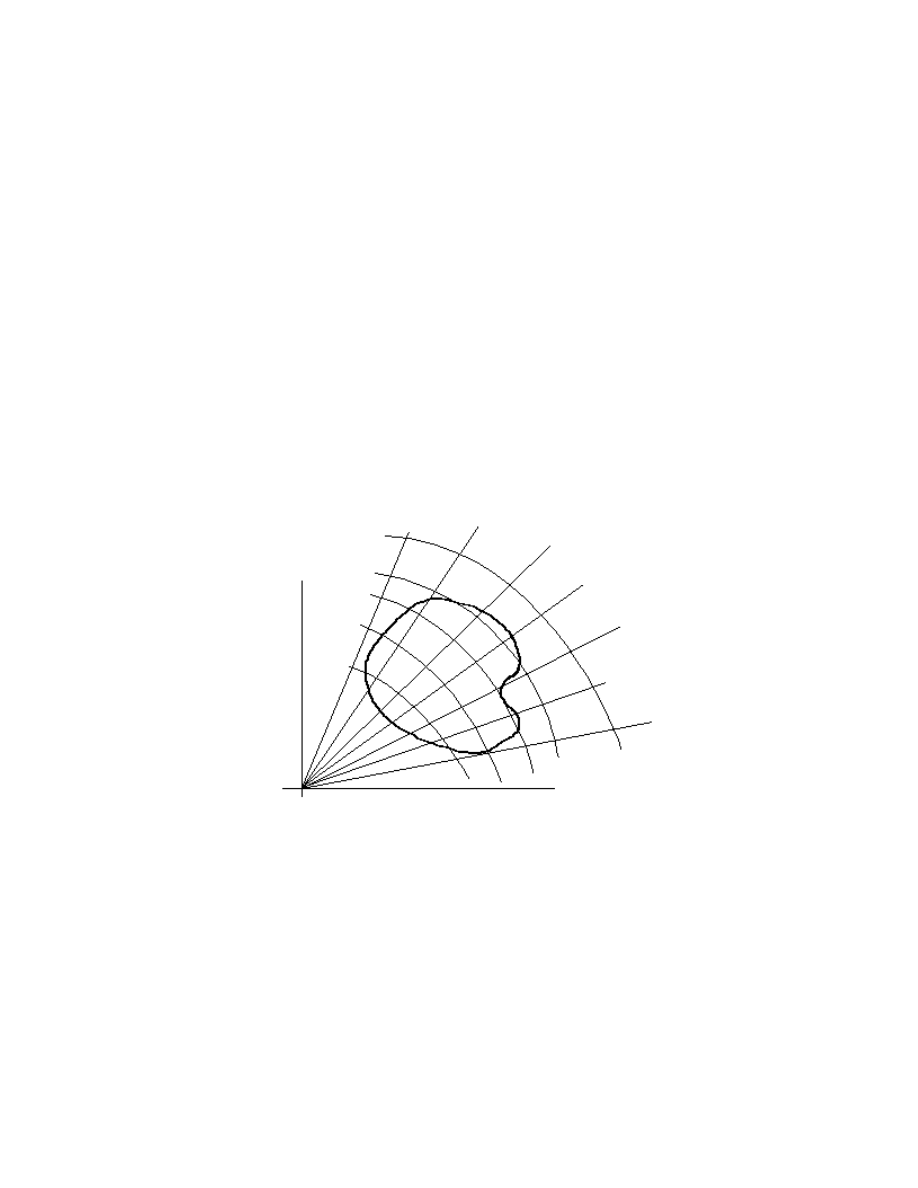
There is, however, more to it than this. When we divided the plane into regions formed

by the curves x

=

constant and y

=

constant , we got rectangles, etc., etc. Now we

divide the plane into regions formed by the curves r

=

constant and

θ =

constant

,

where r and

θ

are the usual polar coordinates. This results in funny shaped regions:

Now, a typical region looks like

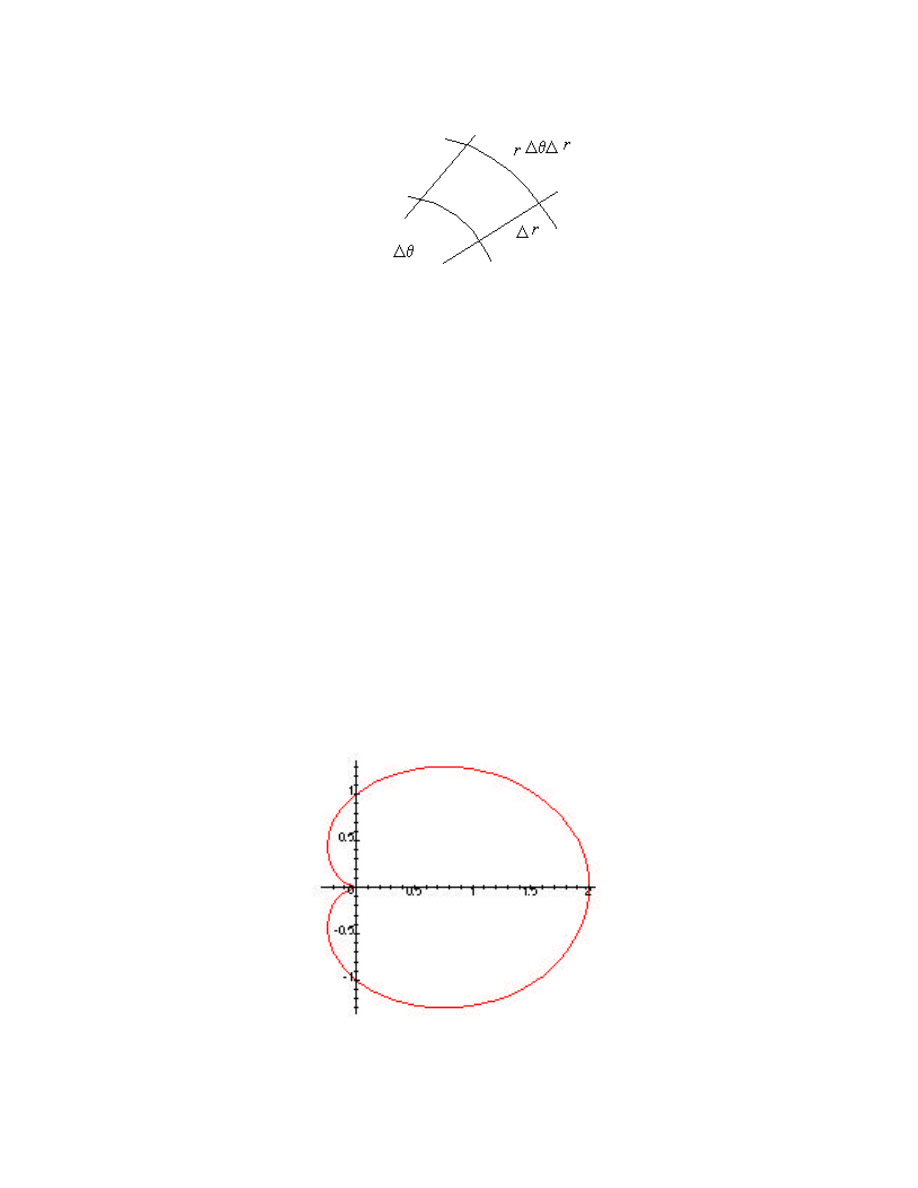
13.7

The area of this region is thus something like

∆

∆ ∆

A

r r

≈

θ

, and our iterated integral looks

like

f x y dA

f r

r

rdrd

( , )

( cos , sin )

D

∫∫

∫∫

=

θ

θ

θ

together with the appropriate limits of integration. (We may, of course, integrate first

with respect to

θ

and then with respect to r if this is convenient.) We desperately need

to see an example.

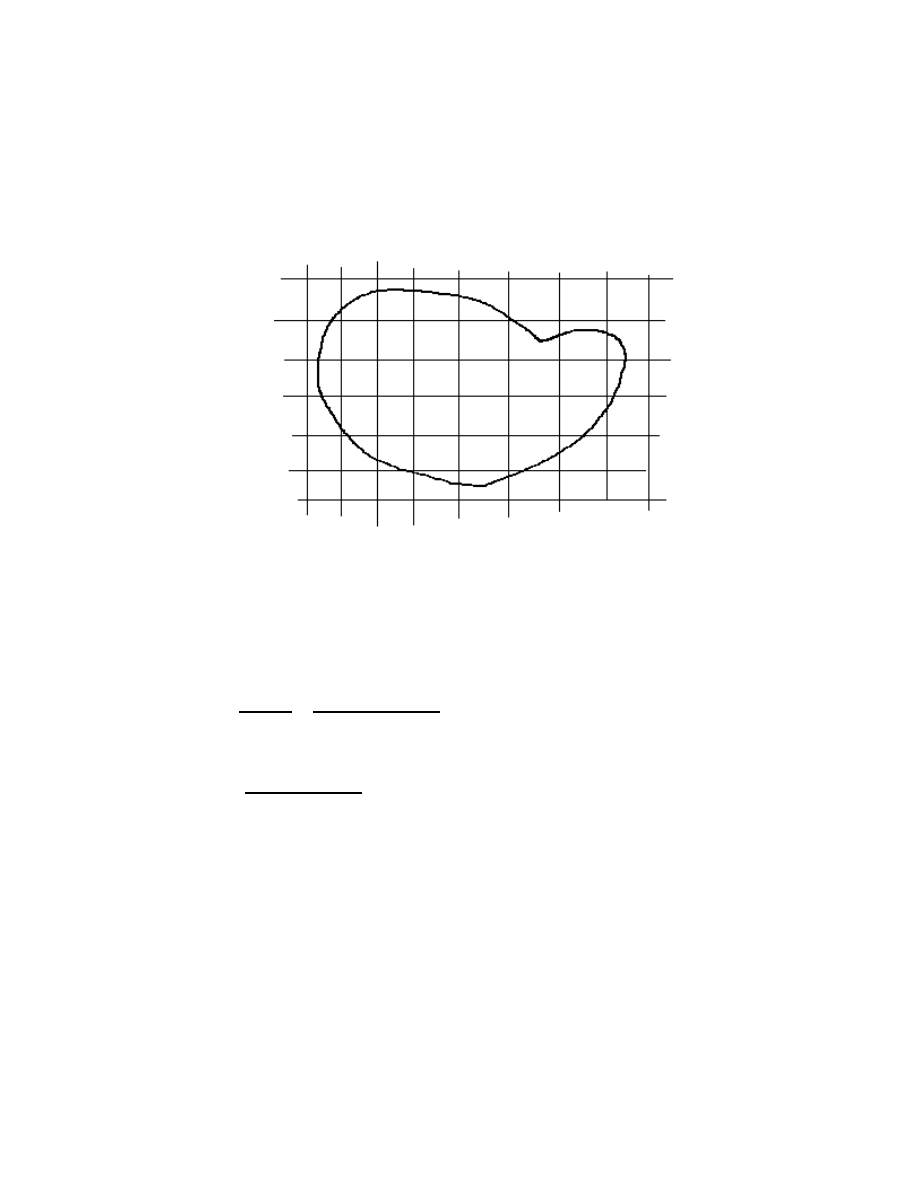
Example

Let's find the centroid of the region enclosed by the curve whose equation in polar

coordinates is

r

= +

1 cos

θ

. Here is a picture drawn by Maple:

13.8

The centroid ( , )

x y is given by

x

xdA

dA

y

ydA

dA

=

=

∫∫

∫∫

∫∫

∫∫

D

D

D

D

, and

.

First. let's find the integral

xdA

D

∫∫

. Now, when we hold

θ

fixed and integrate first with

respect to r, the lower limit is independent of

θ

and is always r

=

0 , while the upper

limit depends, of course on

θ

and is

r

= +

1 cos

θ

. We have a slice for each value of

θ

from

θ =

0

to

θ

π

=

2

, and so our iterated integral looks like

xdA

r

rdrd

r

drd

D

∫∫

∫

∫

∫

∫

=

=

+

+

cos

cos

cos

cos

θ

θ

θ

θ

θ

π

θ

π

0

1

0

2

2

0

1

0

2

.

It is downhill all the way now:

r

drd

d

d

d

d

d

2

0

1

0

2

3

0

2

2

3

4

0

2

0

2

2

0

2

2

0

2

1

3

1

1

3

3

3

1
3

0

3
2

1

2

0

1

4

1

2

6

1

12

2

6

12

15

12

5

4

cos

(

cos ) cos

[cos

cos

cos

cos

]

[

(

cos

)

(

cos

)

]

cos

cos

θ

θ

θ

θ θ

θ

θ

θ

θ θ

θ θ

θ

θ

π

π

θ θ π

π

π

π

π

θ

π

π

π

π

π

π

=

+

=

+

+

+

=

+

+

+ +

+

= + +

= + +

=

=

+

∫

∫

∫

∫

∫

∫

∫

Now for the other integrals.

It should be clear that

ydA

r

drd

D

∫∫

∫

∫

=

=

+

2

0

1

0

2

0

sin

cos

θ

θ

θ

π

. Finally,

13.9

dA

rdrd

d

d

D

∫∫

∫

∫

∫

∫

=

=

+

= +

+

= + =

+

θ

θ

θ

π

θ θ

π

π

π

θ

π

π

π

0

1

0

2

2

0

2

0

2

1

2

1

1

4

1

2

2

3

2

cos

(

cos )

(

cos

)

We are, at last, done.

x

y

=

=

=

5

4

3

2

5

6

0

π

π

,

.

and

Exercises

9. Find the area of the region enclosed by the curve with polar equation

r

=

sin2

θ

.

10. Evaluate the integral

(

)

x

y dA

+

∫∫

D

, where D is the region in the first quadrant inside

the circle x

y

a

2

2

2

+

=

and below the line y

x

=

3 .

11. Find the centroid of the region in the first quadrant inside the circle r

a

=

and between

the rays

θ =

0

and

θ α

=

, where 0

2

≤ ≤

α

π

. What is the limiting position of the

centroid as

α →

0 ?

12. Evaluate

e

dA

x

y

R

2

2

+

∫∫

, where R is the semicircular region bounded above by

y

x

=

−

1

2

and below by the x axis.

13.10

13. Find the area enclosed by one leaf of the rose

r

=

cos3

θ

.

14. Find the area of the region inside

r

= +

1 cos

θ

and outside r

=

1.

13. 3 Three Dimensions

We move along to integrals in three dimensions. The idea is quite simple.

Suppose we have a function f : D

R

→

, where D is a nice subset of R

3

. Capture D

inside a big box (i.e., a rectangular parallelepiped). Now subdivide this box by partitioning

each of its sides. The volume of the largest such box is called the mesh of the subdivision.

In each box that meets D, choose a point (

,

,

)

*

*

*

x y z

i

i

i

in D. A Riemann sum S now looks

like

S

f x y z

V

i

i

i

i

n

i

=

=

∑

(

,

,

)

*

*

*

1

∆

,

where

∆

V

i

is the volume of the box from which (

,

,

)

*

*

*

x y z

i

i

i

was chosen. (The

summation is over all boxes that meet D.) If there is a number L such that |

|

S

L

−

can be

made arbitrarily small by choosing a subdivision of sufficiently small mesh, then we say

that f is integrable over D, and the number L is called the integral of f over D. This

integral is usually written with three snake signs:

f x y z dV

( , , )

D

∫∫∫

.

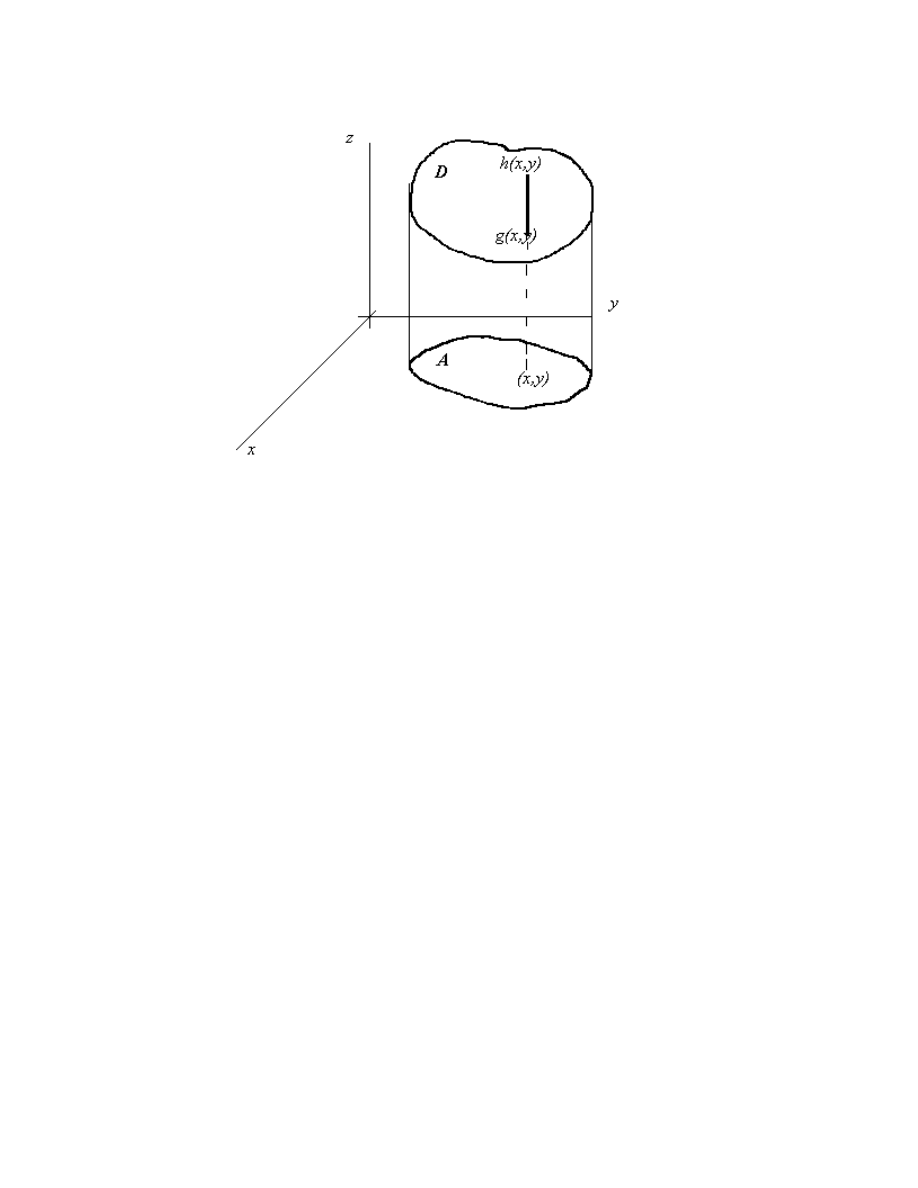
Let's see how to evaluate such a thing by considering iterated integrals. Here's

what we do. First, project D onto a coordinate plane. (We choose the x-y plane as an

example.)

13.11

Let A be the region in the x-y plane onto which D projects. Assume that a vertical line

through a point ( , )

x y

∈

A enters D through the surface z

g x y

=

( , ) and exits through the

surface z

h x y

=

( , ) . In other words, the blob D is the solid above the region A between

the surfaces z

g x y

=

( , ) and z

h x y

=

( , ) . Now we simply integrate the integral

f x y z dz

g x y

h x y

( , , )

( , )

( , )

∫

over the region A:

f x y z dV

f x y z dz dA

g x y

h x y

( , , )

( , , )

( , )

( , )

=











∫

∫∫

∫∫∫

A

D

.

Example

Let's find the integral

(

)

x

y

z dV

+

+

∫∫∫

2

D

, where D is the tetrahedron with vertices

(0,0,0), (1,0,0), (0,2,0), and (0,0,1).

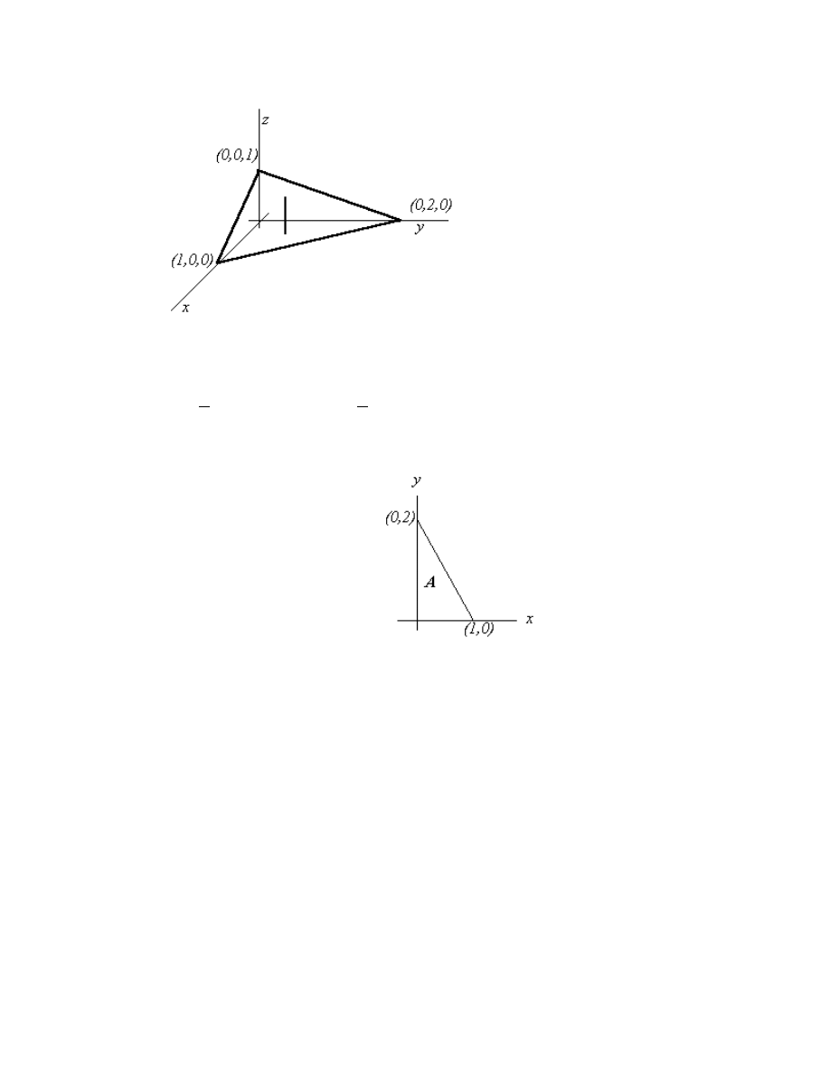
13.12

When we project D onto the x-y plane, the bottom of D is the surface z

=

0 and the top

of D is x

y

z

+ + =

2

1, or z

x

y

= − −

1

2

. The projection is simply the triangle

Our iterated integral is thus simply

(

)

/

x

y

z dz dA

x y

+

+











− −

∫

∫∫

2

0

1

2

A

. We now write the double

integral over A as an iterated integral, and we have

(

)

(

)

/

x

y

z dV

x

y

z dz dA

x y

+

+

=

+

+











− −

∫

∫∫

∫∫∫

2

2

0

1

2

A

D

=

+

+

− −

−

∫

∫

∫

(

)

/

(

)

x

y

z dzdydx

x y

x

2

0

1

2

0

2 1

0

1

.

13.13

Again, it is traditional to omit the parentheses in the iterated integral. All we need do now

is integrate three times. Let's use Maple for the calculations, but look at the intermediate

steps, rather than just use one statement. Here we go.

For the first integration, we want

(

)

/

x

y

z dz

x y

+

+

− −

∫

2

0

1

2

:

int(x+2*y+z,z=0..(1-x-y/2));

Thus,

(

)

/

x

y

z dz

x

xy

y

y

x y

+

+

= −

−

+

−

+

− −

∫

2

1

2

2

3

2

7

8

1

2

0

1

2

2

2

,

and our next integral is

(

)

(

)

(

)

/

(

)

1 2

1

2

2

3

2

7

8

1

2

2

2

0

2 1

0

1

2

0

2 1

+

+

=

−

−

+

−

+

−

− −

−

∫

∫

∫

y

z dzdy

x

xy

y

y

dy

x

x y

x

.

Maple again:

int(-(x^2)/2-2*x*y+(3/2)*y-(7/8)*y^2+1/2,y=0..2*(1-x));

Thus,

(

)

(

)

−

−

+

−

+

= − −

+

+

−

∫

1

2

2

3

2

7

8

1

2

4

2

3

3

5

3

2

2

0

2 1

3

2

x

xy

y

y

dy

x

x

x

x

,

and finally,

int(-4*x-(2/3)*x^3+3*x^2+(5/3),x=0..1);

13.14

At last!

(

)

/

(

)

x

y

z dzdydx

x y

x

+

+

=

− −

−

∫

∫

∫

2

1

2

0

1

2

0

2 1

0

1

.

We make a few obvious observations. First, if S is a solid, the volume V of the

solid is simply V

dV

=

∫∫∫

S

. If the mass density of a blob having the shape of S is

ρ

( , , )

x y z , then the mass M of the blob is M

x y z dV

=

∫∫∫

ρ

( , , )

S

, and the location

( , , )

x y z of the center of mass is given by

x

x

x y z dV

M

=

∫∫∫

ρ

( , , )

S

y

y

x y z dV

M

=

∫∫∫

ρ

( , , )

S

z

z

x y z dV

M

=

∫∫∫

ρ

( , , )

S

Exercises

15. Find the volume of the tetrahedron having vertices (0,0,0), (a,0,0),(0,b,0), and (0,0,c).

16. Find the centroid of the tetrahedron in the previous exercise.

17. Evaluate

(

)

xy

z dV

S

+

∫∫∫

2

, where S is the set S

x y z

z

x

y

=

≤ ≤ − −

{( , , ):

| | | |}

0

1

.

13.15

18. Find the volume of the region in the first octant bounded by the coordinate planes

and the surface z

x

y

= −

−

4

2

.

19. Write six different iterated integrals for the volume of the tetrahedron cut from the

first octant by the plane 12

4

3

12

x

y

z

+

+

=

.

20. A solid is bounded below by the surface z

y

=

4

2

, above by the surface z

=

4 , and on

the ends by the surfaces x

=

1 and x

= −

1. Find the centroid.

21. Find the volume of the region common to the interiors of the cylinders x

y

2

2

1

+

=

and x

z

2

2

1

+

=

.