1.1

Chapter One

Euclidean Three-Space

1.1 Introduction.

Let us briefly review the way in which we established a correspondence between

the real numbers and the points on a line, and between ordered pairs of real numbers and

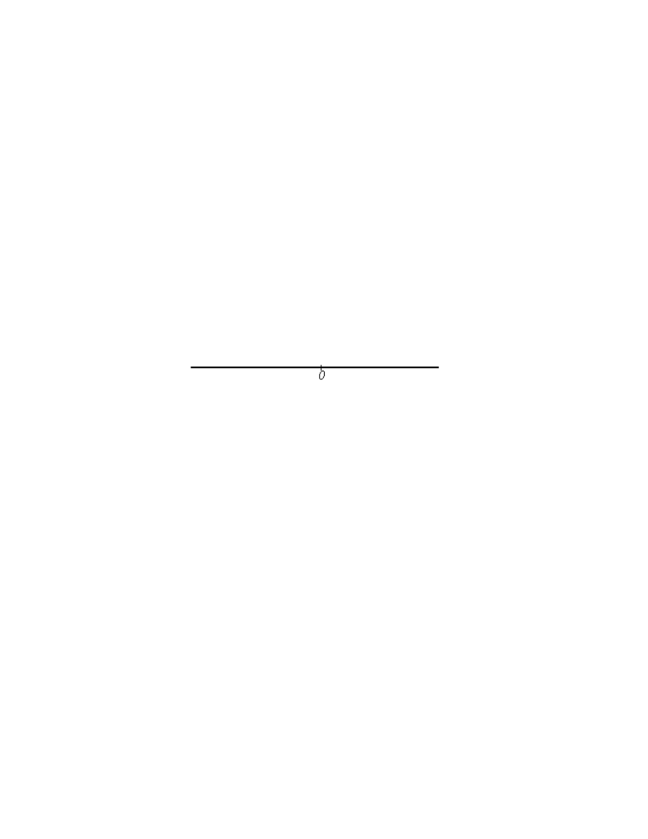
the points in a plane. First, the line. We choose a point on a line and call it the origin.

We choose one direction from the origin and call it the positive direction. The opposite

direction, not surprisingly, is called the negative direction. In a picture, we generally

indicate the positive direction with an arrow or a plus sign:

Now we associate with each real number r a point on the line. First choose some

unit of measurement on the line. For r

>

0, associate with r the point on the line that is a

distance r units from the origin in the positive direction. For r

<

0, associate with r the

point on the line that is a distance r units from the origin in the negative direction. The

number 0 is associated with the origin. A moments reflection should convince you that

this procedure establishes a so-called one-to-one correspondence between the real

numbers and the points on a line. In other words, a real number determines exactly one

point on a line, and, conversely, a point on the line determines exactly one real number.

This line is called a real line.

Next we establish a one-to-one correspondence between ordered pairs of real

numbers and points in a plane. Take a real line, called the first axis, and construct another

real line, called the second axis, perpendicular to it and passing through the origin of the

first axis. Choose this point as the origin for the second axis. Now suppose we have an

ordered pair (

,

)

x x

1

2

of reals. The point in the plane associated with this ordered pair is

1.2

found by constructing a line parallel to the second axis through the point on the first axis

corresponding to the real number x

1

, and constructing a line parallel to the first axis

through the point on the second axis corresponding to the real number

x

2

. The point at

which these two lines intersect is the point associated with the ordered pair (

,

)

x x

1

2

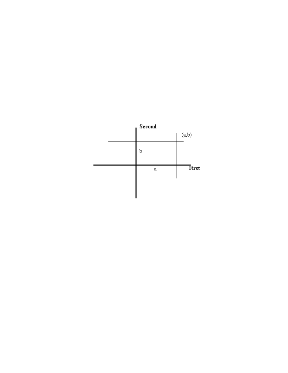
. A

moments reflection here will convince you that there is exactly one point in the plane thus

associated with an ordered pair (a, b), and each point in the plane is the point associated

with some ordered pair (a, b):

It is traditional to assume the point of view we have taken in this picture, in which

the first axis is horizontal, the second axis is vertical, the positive direction on the first

axis is to the right, and the positive direction on the second axis is up. We thus usually

speak of the horizontal axis and the vertical axis, rather than the first axis and the second

axis. We also frequently abuse the language by speaking of a point (

,

)

x x

1

2

when, of

course, we actually mean the point associated with the ordered pair (

,

)

x x

1

2

. The

numbers x

1

and

x

2

are called the coordinates of the point- x

1

is the first coordinate and

x

2

is the second coordinate.

Given any collection of ordered pairs( A collection of ordered pairs is called a

relation.), a picture of the collection is obtained by simply looking at the set of points in

the plane corresponding to the pairs in the given collection. Suppose we have an equation

1.3

involving two variables, say x and y. Then this equation defines a collection of ordered

pairs of numbers, namely all ( , )

x y that satisfy the equation. The corresponding picture

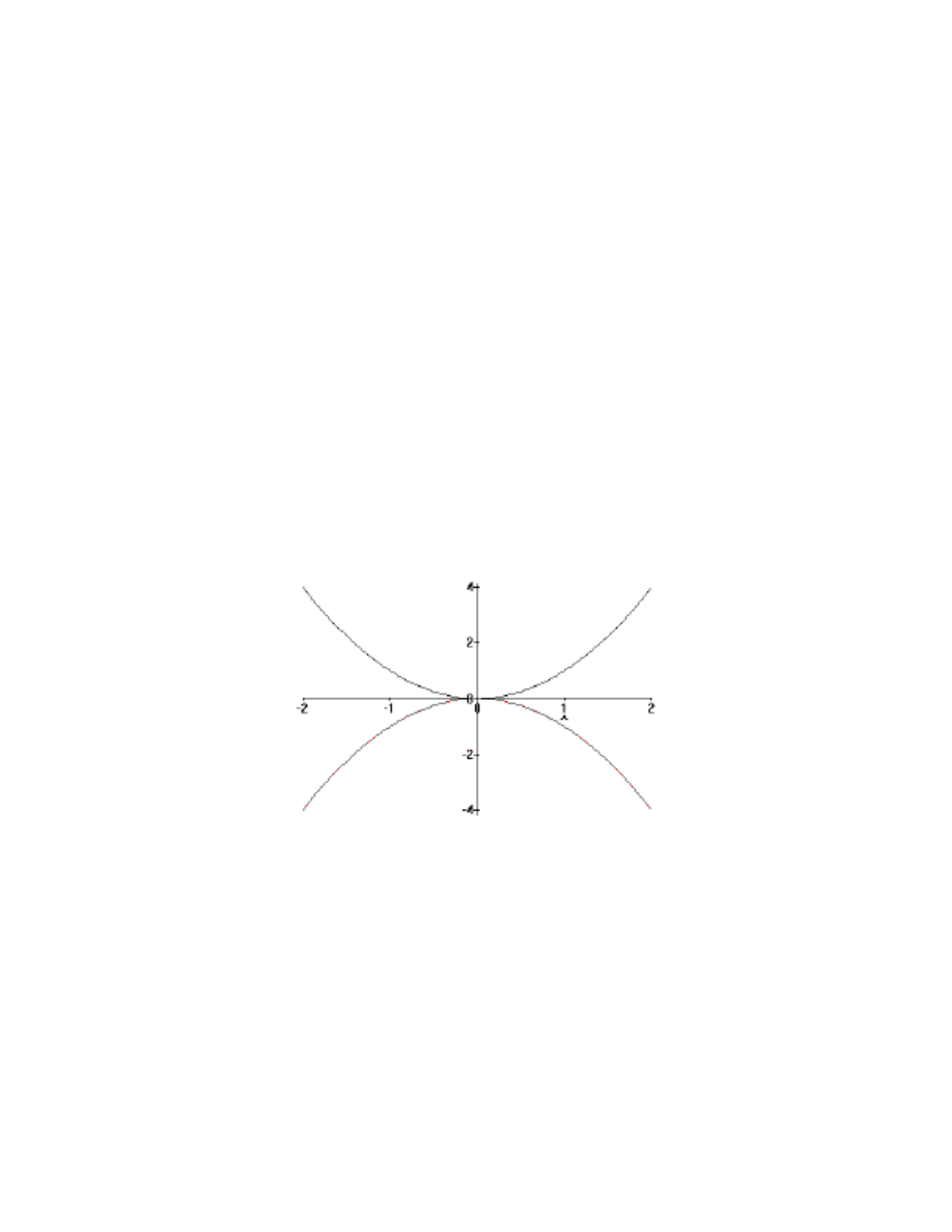
in the plane is called the graph of the equation. For example, consider the equation

y

x

2

4

=

. Let’s take a look at the graph of this equation. A little algebra (very little,

actually), convinces us that

{( , ):

}

{( , ):

}

{( , ):

}

x y y

x

x y y

x

x y y

x

2

4

2

2

=

=

=

∪

= −

,

and we remember from the sixth grade that each of the sets on the right hand side of this

equation is a parabola:

What do we do with all this? These constructions are, of course, the bases of

analytic geometry, in which we join the subjects of algebra and geometry, to the benefit of

both. A geometric figure (a subset of the plane ) corresponds to a collection of ordered

pairs of real numbers. Algebraic facts about the collection of ordered pairs of real are

reflected by geometric facts about the subset of the plane, and, conversely, geometric

1.4

facts about the plane subset are reflected by algebraic facts about the collection of pairs of

reals.

Exercises

Draw a picture of the given relation:

1.

R

x y

x

y

=

≤ ≤

≤ ≤

{( , ):

,

}

0

1

1

4

and

2.

R

x y

x

x

y

x

=

− ≤ ≤

−

≤ ≤

{( , ):

,

}

4

4

2

2

and

3.

R

x y

y

x y y

x

=

≤ ≤ ∩

≥

{( , ):

}

{( , ):

}

1

2

2

4.

S

x y x

y

x

=

+

=

≥

{( , ):

}

2

2

1

0

, and

5.

S

x y x

y

x y y

x

=

+

≤ ∩

≤

{( , ):

}

{( , ):

}

2

2

2

1

6.

E

r s

r

s

=

=

{( , ):| | | |}

7.

T

u v

u

v

=

+ =

{( , ):| | | |

}

1

8.

R

u v u

v

=

+ ≤

{( , ):| | | |

}

1

9.

T

x y x

y

=

=

{( , ):

}

2

2

10. A

x y x

y

=

≤

{( , ):

}

2

2

1.5

11. G

s t

s t

=

=

{( , ):

{| |,| |}

}

max

1

12. B

s t

s t

=

≤

{( , ):

{| |,| |}

}

max

1

1.2 Coordinates in Three-Space

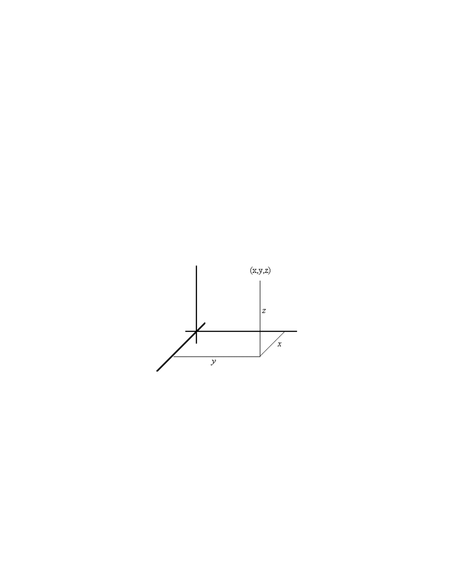
Now let’s see what’s doing in three dimensions. We shall associate with each

ordered triple of real numbers a point in three space. We continue from where we left off

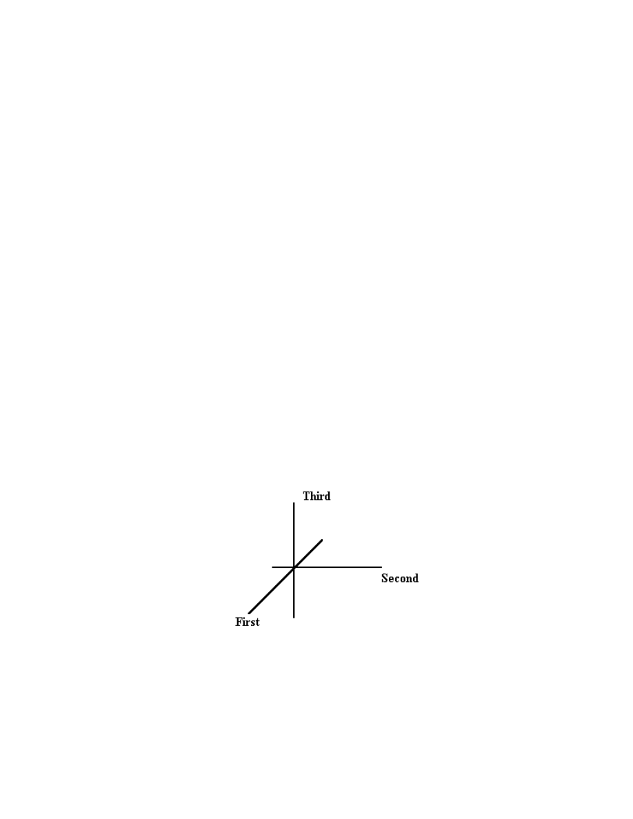
in the previous section. Start with the plane constructed in the previous section, and

construct a line perpendicular to both the first and second axes, and passing through the

origin. This is the third, axis. Now we must be careful about which direction on this

third axis is chosen as the positive direction; it makes a difference. The positive direction

is chosen to be the direction in which a right-hand threaded bolt would advance if the

positive first axis is rotated to the positive second axis:

We now see how to define a one-to-one correspondence between ordered triples

of real numbers (

,

,

)

x x x

1

2

3

and the points in space. The association is a simple extension

of the way in which we established a correspondence between ordered pair and points in

1.6

a plane. Here’s what we do. Construct a plane perpendicular to the first axis through the

point x

1

, a plane perpendicular to the second axis through

x

2

, and a plane perpendicular

to the third axis through x

3

. The point at which these three planes intersect is the point

associated with the ordered triple (

,

,

)

x x x

1

2

3

. Some meditation on this construction

should convince you that this procedure establishes a one-to-one correspondence between

ordered triples of reals and points in space. As in the two dimensional, or plane, case, x

1

is called the first coordinate of the point,

x

2

is called the second coordinate of the point,

and x

3

is called the third coordinate of the point. Again, the point corresponding to

( , , )

0 00 is called the origin, and we speak of the point (

,

,

)

x x x

1

2

3

, when we actually mean

the point which corresponds to this ordered triple.

The three axes so defined is called a coordinate system for three space, and the

three numbers x, y, and z , where ( , , )

x y z is the triple corresponding to the point P, are

called the coordinates of P. The coordinate axes are sometimes given labels-most

commonly, perhaps, the first axis is called the x axis, the second axis is called the y axis,

and the third axis is called the z axis.

1.7

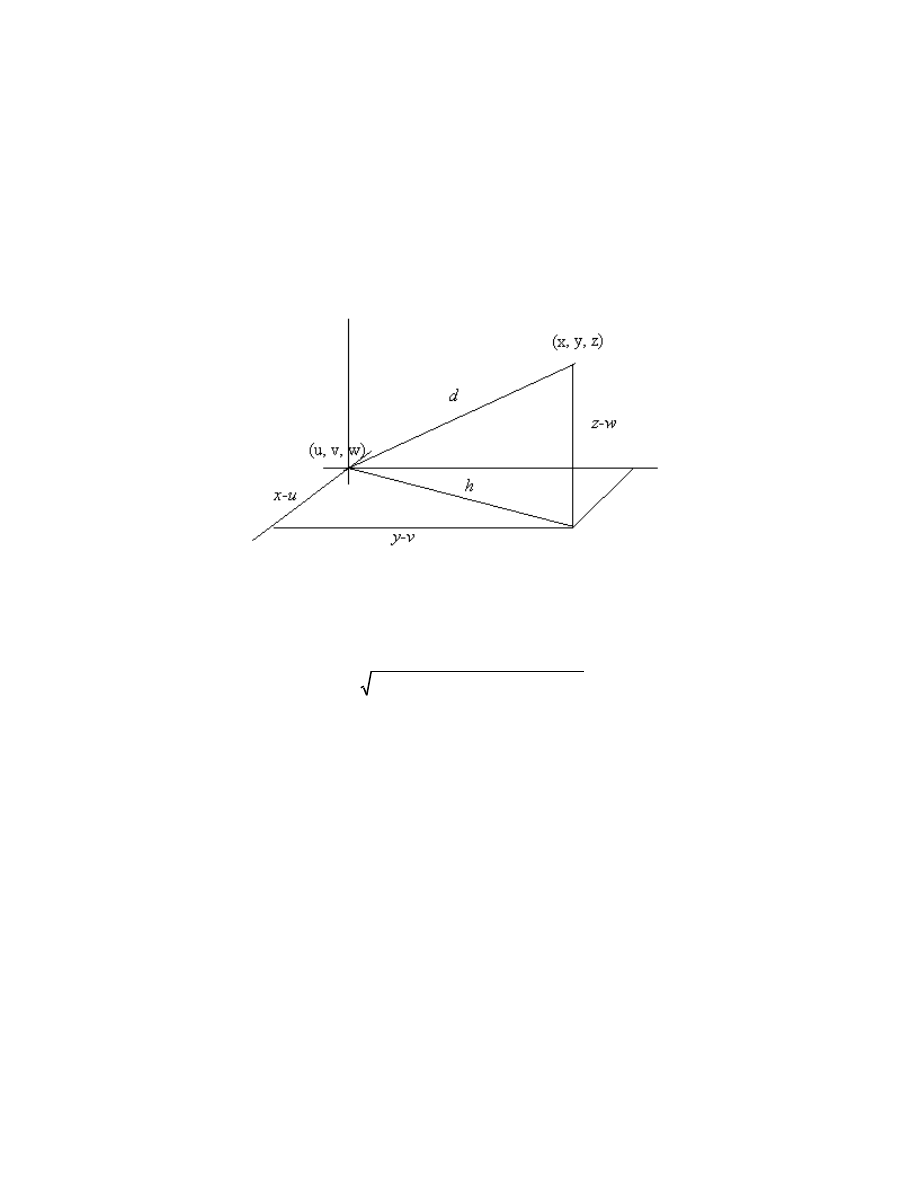
1.3 Some Geometry

Suppose P and Q are two points, and suppose space is endowed with a

coordinate system such that P

x y z

=

( , , ) and Q

u v w

=

( , , ) . How do we find the distance

between P and Q ? This simple enough; look at the picture:

We can see that d

h

z

w

2

2

2

=

+ −

(

) and h

x

u

y

v

2

2

2

=

−

+

−

(

)

(

) . Thus we have

d

x

u

y

v

z

w

2

2

2

2

=

−

+ −

+ −

(

)

(

)

(

) , or

d

x

u

y

v

z

w

=

−

+

−

+ −

(

)

(

)

(

)

2

2

2

.

We saw that in the plane an equation in two variables defines in a natural way a collection

of ordered pairs of numbers. The analogous situation obtains in three-space: an equation

in three variables defines a collection of ordered triples. We thus speak of the collection

of triples ( , , )

x y z which satisfy the equation

x

y

z

2

2

2

1

+

+

=

1.8

The collection of all such points is the graph of the equation. In this example, it is easy

to see that the graph is precisely the set of all points at a distance of 1 from the origin-a

sphere of radius 1 and center at the origin.

The graph of the equation x

=

0 is simply the set of all points with first

coordinate 0, and this is clearly the plane determined by the second axis and the third axis,

or the y axis and the z axis. When the axes are labeled x, y, and z, this is known as the yz

plane. . Similarly, the plane y

=

0 is the xz plane, and z

=

0 is the xy plane. These

special planes are also called the coordinate planes.

More often than not, it is difficult to see exactly what a graph of equation looks

like, and even more difficult for most of us to draw it. Computers can help, but they

usually draw rather poor pictures whose main application is in stimulating your own

imagination sufficiently to allow you to see the graph in your mind’s eye. An example:

This picture was drawn using Maple.

Let’s look at a more complicated example. What does the graph of

x

y

z

2

2

2

1

+

−

=

look like? We’ll go after a picture of this one by slicing the graph with the coordinate

planes. First, let’s slice through it with the plane z

=

0 ; then we see

1.9

x

y

2

2

1

+

=

,

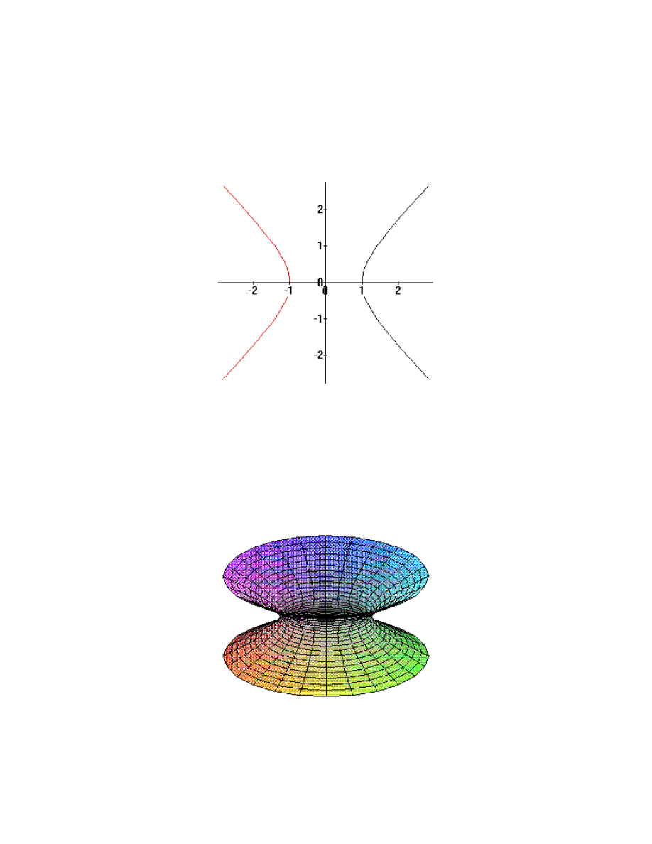
a circle of radius 1 centered at the origin. Next, let’s slice with the plane y

=

0 . Here we

see x

z

2

2

1

−

=

, a hyperbola:

We, of course, see the same hyperbola when we slice the graph with the plane

x

=

0 . What the graph looks like should be fairly clear by now:

1.10

This graph has a name; it is called a hyperboloid.

Exercises

13. Describe the set of points S

x y z x

y

z

=

≥

≥

≥

{( , , ):

,

}

0

0

0

, and

.

14. Describe the following sets

a) S

x y z

=

≥

{( , , ): z

0}

b) S

x y z

x

=

≥

{( , , ):

}

5

c) R

x y z

x

y

=

+

≤

{( , , ):

}

2

2

1

d) T

r s t

r

s

t

=

+

+ ≤

{( , , ):

}

2

2

2

4

15. Let G be the graph of the equation x

y

z

2

2

2

4

9

36

+

+

=

.

a)Sketch the graphs of the curves sliced from G by the coordinate planes x

=

0 ,

y

=

0 , and z

=

0 .

b)Sketch G. (This graph is called an ellipsoid.)

16. Let G be the graph of the equation x

y

z

2

2

2

3

4

12

−

+

=

.

a)Sketch the graphs of the curves sliced from G by the coordinate planes x

=

0 ,

y

=

0 , and z

=

0 .

b)Sketch G. (Does this set look at all familiar to you?.)

1.4 Some More Geometry-Level Sets

The curves that result from slicing the graphs with the coordinate planes are

special cases of what are called level sets of a set. Specifically, if S is a set, the

intersection of S with a plane z

=

constant is called a level set. In case the level set is a

1.11

curve, it is frequently called a level curve. (The slices by planes x = constant, or y =

constant are also level sets.) A family of level sets can provide a nice stimulant to your

powers of visualization. Everyday examples of the use of level sets to describe a set are

contour maps, in which the contours are, of course, just level curves ; and weather maps,

in which, for instance, the isoclines on a 500mb chart are simply level curves for the

500mb surface. Let’s illustrate with an example.

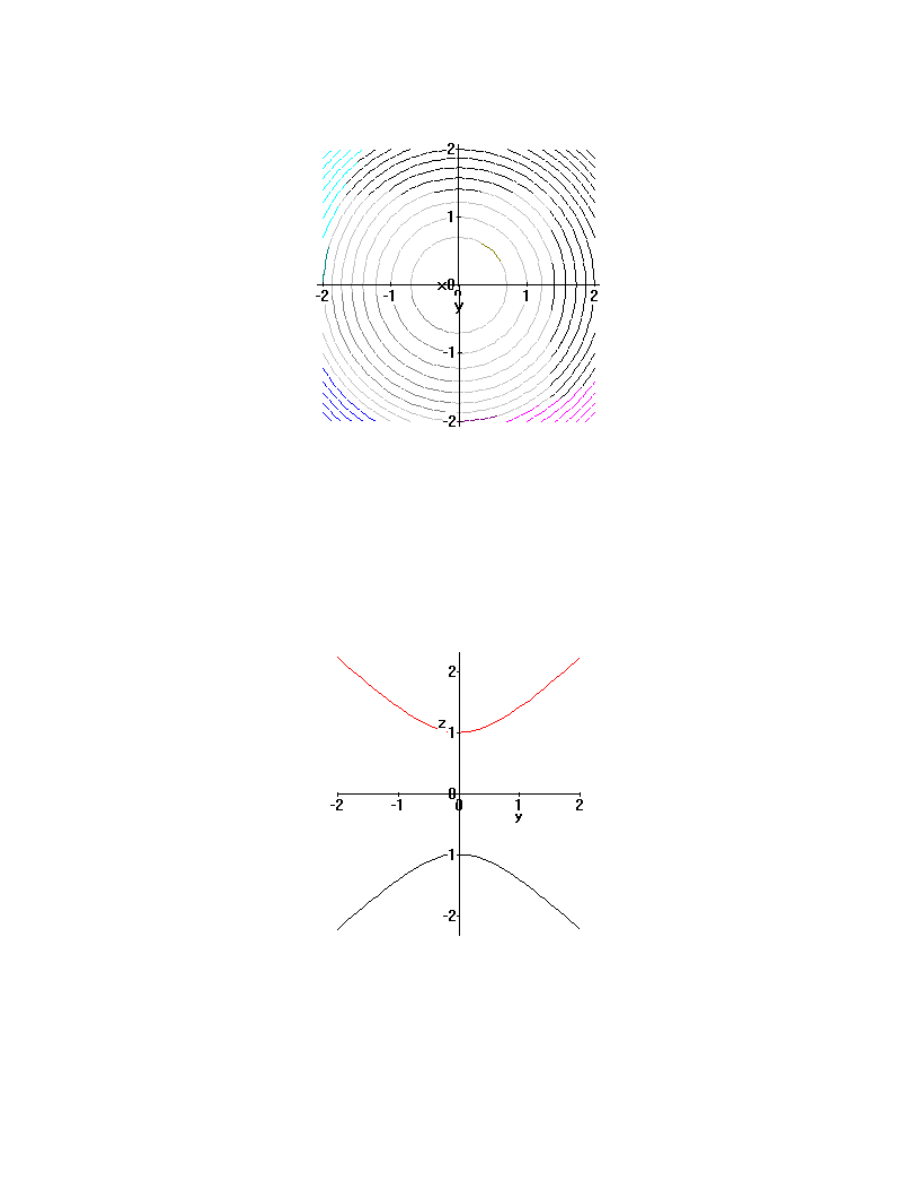
Let S be the graph of

z

y

x

2

2

2

1

−

−

=

Now we look at the level set z

c

=

:

c

y

x

2

2

2

1

−

−

=

, or

x

y

c

2

2

2

1

+

=

−

.

Notice first that we have the same curve for z = c and z = -c. The graph is symmetric

about the plane z = 0. We shall thus look at just that part of the graph that is above the

xy plane.

It is clear that these curves are concentric circles of radius

c

2

1

−

centered at the

origin. There are no level sets for | |

c

<

1, and for c = 1 or -1, the level set is a single point,

the origin.

1.12

Next, slice with the planes x = 0 and y = 0 to get a better idea of what this thing

looks like. For x = 0, we see

z

y

2

2

1

−

=

,

a hyperbola:

The slice by y = 0, of course, is the same. It is rather easy to visualize this graph. Here is

a Maple drawn picture:

1.13

This also is called a hyperboloid. This is a hyperboloid of two sheets, while the

previously described hyperboloid is a hyperboloid of one sheet.

Exercises

17. Let S

x x x

x

x

x

=

+

+

=

{(

,

,

):|

| |

| |

|

}

1

2

3

1

2

3

1 .

a)Sketch the coordinate plane slices of S.

b)Sketch the set S.

18. Let C be the graph of the equation z

x

y

2

2

2

4

=

+

(

) .

a)Sketch some level sets z = c.

b)Sketch the slices by the planes x = 0 and y = 0.

c)Sketch C. What does the man on the street call this set?

19. Using level sets, coordinate plane slices, and whatever, describe the graph of the

equation z

x

y

=

+

2

2

. (This one has a name also; it is a paraboloid.).

1.14

20. Using level sets, coordinate plane slices, and whatever, describe the graph of the

equation z

x

y

=

−

2

2

.