17.1

Chapter Seventeen

Gauss and Green

17.1 Gauss's Theorem

Let B be the box, or rectangular parallelepiped, given by

B

=

≤ ≤

≤ ≤

≤ ≤

{( , , ):

,

,

}

x y z x

x

x

y

y

y

z

z

z

0

1

0

1

0

1

;

and let S be the surface of B with the orientation that points out of B. Let F B

R

3

:

→

be

a nice function, or field. For reasons that will become apparent as the drama unfolds, let's

compute the flux

F r

S

( )

⋅

∫∫

d

S

.

We shall do this by computing the surface integral over each of the six sides of B

and adding the results. Let S

1

be the side in the plane x

x

=

1

; let S

2

be the side in the

plane x

x

=

0

; let S

3

be the side in the plane y

y

=

1

; let S

4

be the side in the plane

y

y

=

0

; and let S

5

and S

6

be the obvious things. We begin by computing the integral

F r

S

( )

⋅

∫∫

d

S

1

.

A vector description of S

1

is quite easy to come by; it is, of course, simply

r

i

j

k

( , )

s t

x

s

t

=

+ +

1

,

where y

s

y

0

1

≤ ≤

and z

t

z

0

1

≤ ≤

. (Obviously, s is simply y, and t is z .) Then

∂
∂

∂
∂

s

r

r

j

k

i

×

= × =

t

.

It is clear this is the specified orientation. If F r

i

j

k

( )

( , , )

( , , )

( , , )

=

+

+

p x y z

q x y z

r x y z

,

then

F r

S

F

i

( )

(

, , )

(

, , )

⋅

=

⋅

=

∫

∫

∫∫

∫

∫

d

x s t

dtds

p x s t dtds

z

z

y

y

S

z

z

y

y

1

1

0

1

0

1

1

0

1

0

1

17.2

A vector description for the opposite side, x

x

=

0

, is just

r

i

j

k

( , )

s t

x

s

t

=

+ +

0

,

and we have

F r

S

F

i

( )

(

, , ) (

)

(

, , )

⋅

=

⋅ −

=

−

∫

∫

∫∫

∫

∫

d

x s t

dtds

p x s t dtds

z

z

y

y

S

z

z

y

y

0

0

0

1

0

1

2

0

1

0

1

The sum of these two is then

F r

S

F r

S

( )

( )

⋅

+

⋅

=

∫∫

∫

∫

∫∫

d

d

dtds

S

z

z

y

y

S

1

0

1

0

1

2

[p(x , s, t) - p(x , s, t)]

1

0

.

Observe that

p x s t

p x s t

p

x

s t d

x

x

(

, , )

(

, , )

( , , )

1

0

0

1

−

=

∫

∂
∂

ξ

ξ

.

Substitution of this into the previous equation gives us

F r

S

F r

S

( )

( )

( , , )

⋅

+

⋅

=

=

∫∫

∫

∫

∫

∫∫

∫∫∫

d

d

p

x

s t d dtds

p

x

dV

S

x

x

z

z

y

y

S

B

10

0

1

0

1

0

1

21

∂
∂

ξ

ξ

∂
∂

and we have turned the sum of the two surface integrals into a plain ol' volume integral .

It should be clear how we also obtain

F r

S

F r

S

( )

( )

⋅

+

⋅

=

∫∫

∫∫

∫∫∫

d

d

q

y

dV

S

S

B

3

4

∂
∂

, and

F r

S

F r

S

( )

( )

⋅

+

⋅

=

∫∫

∫∫

∫∫∫

d

d

r

z

dV

S

S

B

5

6

∂
∂

.

17.3

The flux over the entire surface S is thus the sum of these:

(

z)

F r

S

( )

⋅

=

+

+

=

+

+











∫∫∫

∫∫

∫∫∫

∫∫∫

∫∫∫

d

p

dV

q

dV

r

dV

p

q

r

dV

B

S

B

B

B

∂
∂

∂
∂

∂
∂

∂
∂

∂
∂

∂
∂

x

y

z

x

y

z

We have now found the surface integral, or flux, in terms of an ordinary volume integral.

Now, suppose we have an "arbitrary" solid region B bounded by a surface S,

together with a function F r

i

j

k

( )

( , , )

( , , )

( , , )

=

+

+

p x y z

q x y z

r x y z

defined on

B. Trap

B in a box and subdivide the box into parallelepipeds. Consider those parallelepipeds

{ :

, ,

, }

B i

n

i

=

1 2

K

that meet B. The surface that bounds B

i

will be called S

i

, and oriented

so that the normal points out. The union P

n

i

B

= ∪

{ } of all the B

i

is thus an

approximation to the original solid B.

Apply the equation (

z) to each of these and sum the equations:

F r

S

( )

⋅

=

+

+











∫∫

∑

∫∫∫

∑

d

p

q

r

dV

S

i

B

i

i

i

∂
∂

∂
∂

∂
∂

x

y

z

.

The sum on the right hand side is just the integral over P

n

:

F r

S

( )

⋅

=

+

+











∫∫

∑

∫∫∫

d

p

q

r

dV

S

i

P

i

ni

∂
∂

∂
∂

∂
∂

x

y

z

.

Take a closer look at the sum of the surface integrals on the left hand side of this

equation. Suppose parallelepipeds B

j

and B

k

are adjacent, and call the common side T :

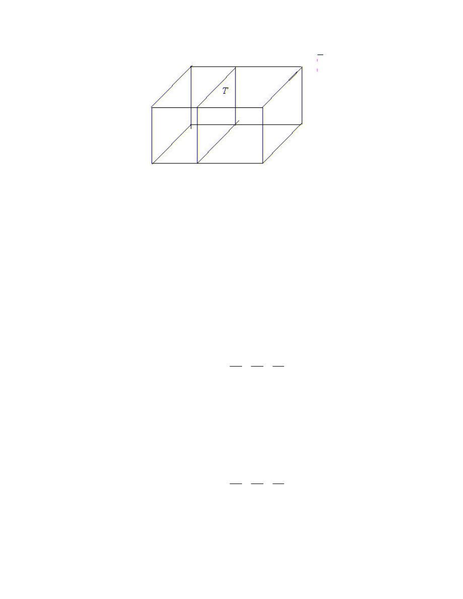
17.4

In the sum of surface integrals, the integral over the common side T appears twice, once

from the integral over S

j

, the surface of B

j

and once from the integral over S

k

, the

surface of B

k

. These integrals, will, however, have opposite signs because the

orientation of T has one direction as a part of the surface of B

j

and the opposite direction

as a part of the surface of B

k

. These two terms thus sum to zero and cancel each other.

In the sum of all the surface integrals, we are therefore left with only the integrals over

sides that are not adjacent to another box. A moments reflection, and you see that what is

left is precisely the integral over the boundary S

n

of P

n

with the outward pointing

orientation. Mirabile dictu, this is precisely the equation (

z):

F r

S

( )

⋅

=

+

+











∫∫∫

∫∫

d

p

q

y

r

z

dV

P

S

n

n

∂
∂

∂
∂

∂
∂

x

.

Now, as everyone can see coming, we look at the limit of this equation as we take smaller

and smaller subdivisions. Then P

B

n

→

and S

S

n

→

, giving us precisely the same result

for the arbitrary region B:

F r

S

( )

⋅

=

+

+











∫∫∫

∫∫

d

p

q

y

r

z

dV

B

S

∂
∂

∂
∂

∂
∂

x

.

17.5

This is really a big deal—such a big deal that it has its own name. This is called Gauss's

Theorem, or the Divergence Theorem.

The integrand in the volume integral also has a name; it is called the divergence of

the function F. It is usually designated either div F , or

∇ ⋅

F . Thus,

div

p

x

q

y

r

z

F

F

= ∇ ⋅

=

+

+

∂
∂

∂
∂

∂
∂

.

With this new definition, Gauss’s Theorem looks like

dV

d

S

∫∫

∫∫∫

⋅

∇

=

⋅

)

(

)

(

r

F

S

r

F

Example

Let's find the divergence of F r

r

r

( )

| |

=

c

3

. First we need to see F in the form

F

i

j

k

( , , )

( , , )

( , , )

( , , )

x y z

p x y z

q x y z

r x y z

=

+

+

.

That's easy:

F

i

j

k

=

+

+

+ +

c

x

y

z

x

y

z

(

)

[

]

/

2

2

2

3 2

,

and so

p

cx

x

y

z

=

+

+

(

)

/

2

2

2

3 2

,

q

cy

x

y

z

=

+

+

(

)

/

2

2

2

3 2

,

r

cz

x

y

z

=

+

+

(

)

/

2

2

2

3 2

.

A bit of elementary school calculus (remember Mrs. Turner!), and we have

17.6

∂
∂

p

x

c

x

y

z

x

x

y

z

=

+

+

−

+

+

2

2

2

2

2

2

2

5 2

3

(

)

/

,

∂
∂

q

y

c

x

y

z

y

x

y

z

=

+

+

−

+

+

2

2

2

2

2

2

2

5 2

3

(

)

/

,

∂
∂

r

z

c

x

y

z

z

x

y

z

=

+

+

−

+

+

2

2

2

2

2

2

2

5 2

3

(

)

/

.

Hence,

∇ ⋅ =

F

0 everywhere (except, of course, for r = 0, where F is not defined.).

Gauss's Theorem now tells us that the integral of F over any closed surface that

does not enclose r = 0 must be zero. This might be the ho-hum of the week save for the

fact that the function F is a common one. It is the gravitational field of a point mass fixed

at the origin, or the electric intensity field for a point charge fixed at the origin, or any field

in which the magnitude is inversely proportional to the distance from the origin and which

points in the direction of the origin.

Exercises

1. Find the outward flux of the function F

i

j

k

=

−

+ −

+

−

(

)

(

)

(

)

y

x

z

y

y

x

across the

boundary of the cube bounded by the planes x

= ±

4 , y

= ±

4 , and z

= ±

4 .

2. Find

[

]

y

xy

z

d

S

i

j

k

S

+

−

⋅

∫∫

, where S is the boundary of the solid inside the cylinder

x

y

2

2

1

+

≤

between z = 0 and z

x

y

=

+

2

2

, with the outward pointing orientation.

3. Find

[log(

)

tan

]

x

y

z

x

y

x

z x

y

d

S

2

2

1

2

2

2

+

+ 







+

+

⋅

−

∫∫

i

j

k

S , where S is the boundary of

the solid {( , , ):

,

}

x y z

x

y

z

1

2

1

2

2

2

≤

+

≤

− ≤ ≤

.

17.7

4. Let B a region in R

3

, and let f : B

R

→

be a function such that

∂
∂

∂
∂

∂

∂

2

2

2

2

2

2

0

f

x

f

y

f

z

+

+

=

in B (Such a function f is said to be harmonic in B.). Let S

be the boundary of B. Show that

∇ ⋅

=

∫∫

f d

S

S

0 .

17.2 Green's Theorem

Let R be the rectangular region in the plane bounded by the rectangle with vertices

(

,

),(

,

), (

,

),

x y

x y

x y

0

0

1

0

1

1

and (

,

)

x y

0

1

.

(

,

)

x y

0

1

)

,

(

1

1

y

x

(

,

)

x y

0

0

( ,

)

x y

1

0

Suppose F

R

2

: R

→

is a vector function given by F

i

j

( , )

( , )

( , )

x y

p x y

q x y

=

+

. Now,

let's compute the vector line integral of F around the rectangular boundary C in the

counterclockwise direction. We shall compute the integral in four parts: the integrals

along each of the straight line segments making up the boundary.

C

3

←

C

4

↓

↑

C

2

→

C

1

Thus,

17.8

F

r

F

r

F

r

F

r

F

r

C

2

⋅

=

⋅ +

⋅ +

⋅ +

⋅

∫

∫

∫

∫

∫

d

d

d

d

d

C

C

C

C

1

3

4

.

We shall work out the evaluation of one of these in some painful detail; it should then be

rather obvious how to do the others. Start with a vector description of C

1

:

r

i

j

( )

t

t

y

= +

0

, x

t

x

0

1

≤ ≤

.

Then, of course,

d

dt

r

i

=

, and our line integral becomes

F

r

i

j

i

⋅

=

+

⋅

=

∫

∫

∫

d

p t y

q t y

dt

p t y dt

x

x

C

x

x

[ ( ,

)

( ,

) ]

( ,

)

0

0

0

0

1

1

0

1

.

In a similar fashion, we get

F

r

⋅

= −

∫

∫

d

p t y dt

C

x

x

3

0

1

1

( ,

)

.

Thus,

F

r

F

r

⋅ +

⋅

= −

−

=

−

= −

∫

∫

∫

∫

∫

∫∫

d

d

p t y

p t y

dt

p

y

t s dsdt

p

y

dA

C

C

x

x

y

y

x

x

R

3

1

0

1

0

1

0

1

1

0

[ ( ,

)

( ,

)]

( , )

∂
∂

∂
∂

In essentially the same manner, we find that

F

r

F

r

⋅ +

⋅

=

∫

∫

∫∫

d

d

q

x

dA

C

C

R

2

4

∂
∂

.

17.9

Thus

F

r

F

r

F

r

F

r

F

r

C

2

⋅

=

⋅ +

⋅ +

⋅ +

⋅

=

−











∫

∫

∫

∫

∫

∫∫

d

d

d

d

d

q

x

p

y

dA

C

C

C

C

R

1

3

4

∂

∂

∂
∂

We have turned a one dimensional vector integral into a double integral, similar to

the way in which in the previous section we turned a two dimensional vector integral into

a triple integral.

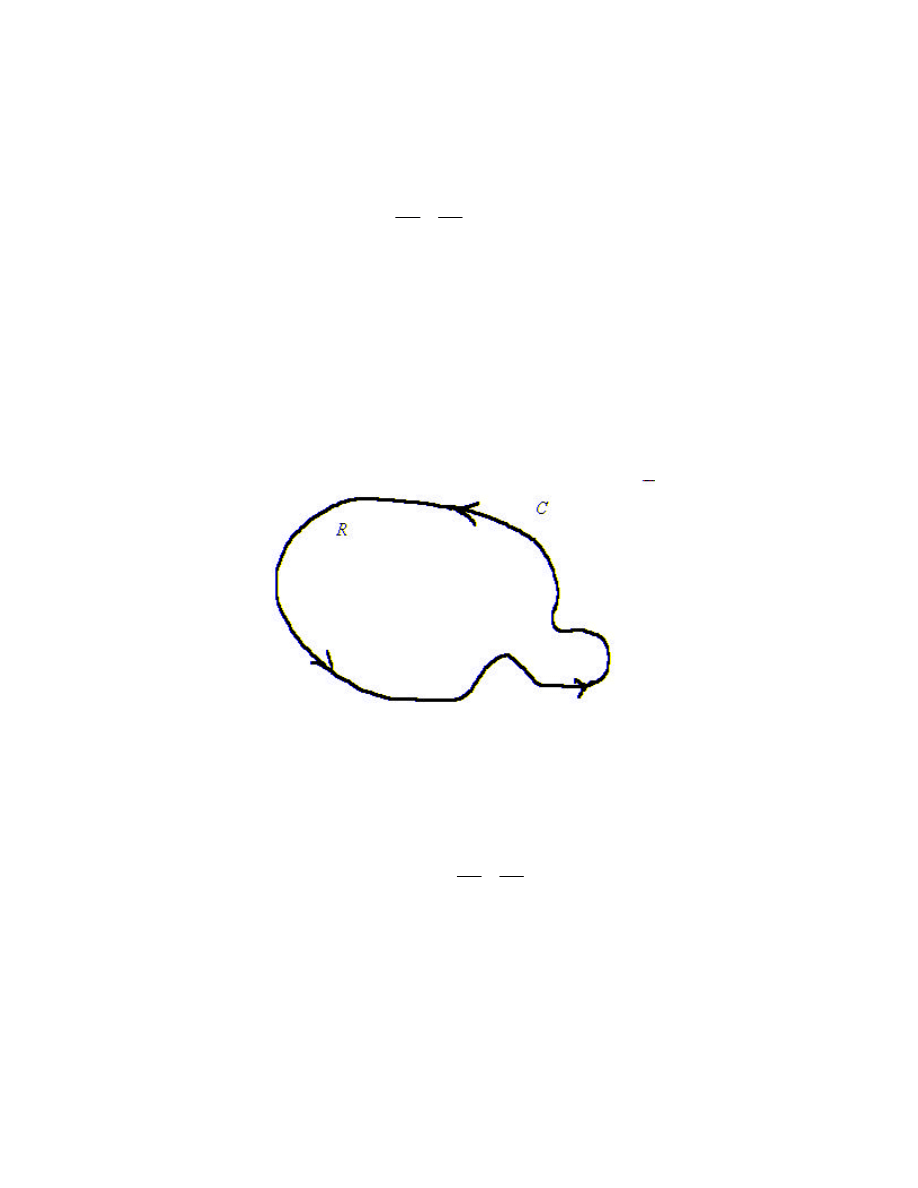
Now suppose we have a reasonable region R bounded by a reasonable curve C

with a counterclockwise orientation:

Now cover this region with rectangles, and apply the above recipe to each rectangle, and

add all the equations, etc., etc., just as we did with the parallelepipeds in deriving Gauss's

Theorem. When the dust settles, we have the same result:

F

r

⋅

=

−











∫

∫∫

d

q

x

p

y

dA

C

R

∂

∂

∂
∂

.

This is called Green's Theorem. You should note that the same equation is valid even if

the region R is bounded by more than one closed curve.

17.10

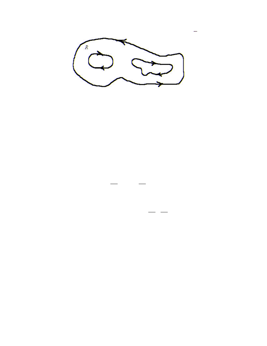
Here the boundary C consists of three curves with the orientation indicated by the arrows

in the fine picture—meditate on the covering by approximating rectangles and you will see

why the orientation of the "inside" curves is clockwise. The line integral on the left side is

simply the sum of the integrals over the pieces of the boundary curve.

Example

Let's evaluate the line integral [

(

) ]

5

3

1

y

x

d

C

i

j

r

+

+

⋅

∫

, where C is the circle of

radius 2 centered at the origin, oriented counterclockwise. First, note that

∂
∂

∂
∂

x

, and

q

p

y

=

=

3

5 .

Thus,

[

(

) ]

5

3

1

2

8

y

x

d

q

x

p

y

dA

dA

C

R

R

i

j

r

+

+

⋅

=

−











= −

= −

∫

∫∫

∫∫

∂

∂

∂
∂

π

Exercises

5. Evaluate [(sin

)

(

) ]

x

y

x

e

d

y

C

+

+

−

⋅

−

∫

3

2

2

2

i

j

r , where C is the boundary of the half-disc

x

y

y

2

2

9

0

+

≤

≥

,

oriented counterclockwise.

17.11

6. Evaluate

(tan

)

log(

)

−

+

+







⋅

∫

1

2

2

y

x

x

y

d

C

i

j

r , where C is the boundary of the region

1

2 0

≤ ≤

≤ ≤

r

,

θ π , oriented clockwise. (These are the usual polar coordinates.)

7. Evaluate the line integral [

]

ye

x e

d

x

y

C

2

3

i

j

r

+

⋅

∫

, where C is the curve given by

r

i

j

( )

sin

sin

,

t

t

t

t

=

+

≤ ≤

2

0

2

π by using Green's Theorem.

17.3 A Pleasing Application

Here we shall use Green’s Theorem to find the area of a region R bound by a

polygon P with vertices

).

,

(

,

),

,

(

),

,

(

2

2

1

1

n

n

y

x

y

x

y

x

K

How do we do this? We simply

apply Greens’ Theorem to the function

j

j

i

F

x

y

x

q

y

x

p

y

x

=

+

=

)

,

(

)

,

(

)

,

(

.

Then Green’s Theorem tells us that

∫

∫∫

⋅

=













∂

∂

−

∂

∂

P

R

d

y

x

dA

x

p

x

q

r

F

)

,

(

,

which becomes

r

j d

x

dA

R

P

∫∫

∫

⋅

=

.

We thus find the area by evaluating the line integral on the right side. This is easy. We

simply integrate over each line segment of the polygon and add up the integrals.

Let’s integrate along the line segment L

k

from

)

,

(

k

k

y

x

to

)

,

(

1

1

+

+

k

k

y

x

. A vector

description of this segment is

)

(

)

)(

1

(

)

(

1

1

j

i

j

i

r

+

+

+

+

+

−

=

k

k

k

k

y

x

t

y

x

t

t

,

1

0

≤

≤

t

.

Thus

j

i

r

)

(

)

(

)

(

'

1

1

k

k

k

x

y

y

x

x

t

−

+

−

=

+

+

, and we have

17.12

2

)

)(

(

]

)

1

[(

)

(

)

(

'

]

)

1

[(

1

1

1

0

1

1

1

0

1

k

k

k

k

k

k

k

k

L

k

k

x

x

y

y

t

d

tx

x

t

y

y

dt

t

tx

x

t

d

x

k

+

−

=

+

−

−

=

⋅

+

−

=

⋅

+

+

+

+

+

∫

∫

∫

r

j

r

j

Thus, Area =

2

)

)(

(

2

)

)(

(

1

1

1

1

1

1

n

n

n

k

k

k

k

k

R

x

x

y

y

x

x

y

y

dA

+

−

+

+

−

=

∑

∫∫

−

=

+

+

.

Meditate on this result. It is really a very simple formula for the area enclosed by a

polygon.

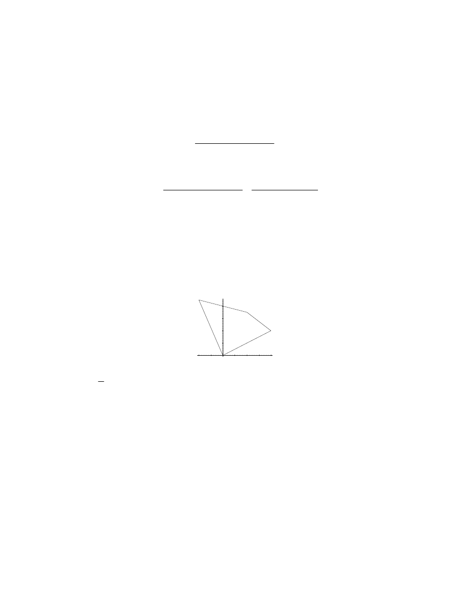
Example. We shall find the area of the quadrilateral with vertices (0, 0), (2, 4), (1, 7),

and (-1, 9):

0

2

4

6

8

-1

-0.5

0.5

1

1.5

2

x

Area =

[

]

4

)]

0

1

)(

0

9

(

)

1

1

)(

7

9

(

)

1

2

)(

4

7

(

)

0

2

)(

0

4

(

2

1

=

+

−

−

+

+

−

−

+

+

−

+

+

−

Exercises

8. Find the area enclosed by the octagon with vertices (0, 0), (1, 0), (2, 3), (0, 5), (-2, 2),

(-1, -1), (-2, -2), (-1, -3).

9. By means of a clever choice of the function

)

,

(

y

x

F

, use Green’s Theorem and derive a

recipe for the integral

∫∫

R

xdA , where R is the region enclosed by the polygon with

vertices

).

,

(

,

),

,

(

),

,

(

2

2

1

1

n

n

y

x

y

x

y

x

K

17.13

10. By means of a clever choice of the function

)

,

(

y

x

F

, use Green’s Theorem and derive

a recipe for the integral

∫∫

R

ydA , where R is the region enclosed by the polygon with

vertices

).

,

(

,

),

,

(

),

,

(

2

2

1

1

n

n

y

x

y

x

y

x

K

11. Find the centroid of the region enclosed by the triangle with vertices (1, 1), (2, 8), and

(5, 5).