18.1

Chapter Eighteen

Stokes

18.1 Stokes's Theorem

Let F

R

3

: D

→

be a nice vector function. If

F

i

j

k

( , , )

( , , )

( , , )

( , , )

x y z

p x y z

q x y z

r x y z

=

+

+

,

the curl of F is defined by

curl

r

y

q

z

p

z

r

x

q

x

p

y

F

i

j

k

=

−









 +

−









+

−











∂
∂

∂

∂

∂

∂

∂
∂

∂

∂

∂
∂

.

Here also the so-called del operator

∇ =

+

+

i

j

k

∂

∂

∂

∂

∂

∂

x

y

z

provides a nice

memory device:

curl

x

y

z

p

q

r

F

F

i

j

k

= ∇ × =

∂

∂

∂

∂

∂

∂

.

This definition allows us to look at Green's Theorem from a new perspective by

observing that in case F

i

j

( , )

( , )

( , )

x y

p x y

q x y

=

+

, Green's Theorem becomes

(

♥

) F

r

F

S

⋅

=

⋅

∫∫

∫

d

curl

d

R

C

,

where we are thinking of the region R as an oriented surface with its orientation pointing

in the direction of k.

We want to look at this formula in case the region R is not necessarily in the i-j

plane, in which case, the word "clockwise" doesn't help in deciding on the orientation of

the boundary C. Once again, we orient things according to our familiar "right-hand" rule.

18.2

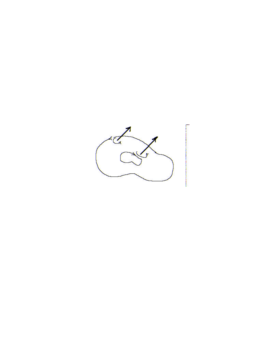
Here's the way it goes. Suppose now S is any surface bounded by a finite number of

disjoint curves C C

C

n

1

2

,

,

K

. We say simply that C

C

C

C

n

=

∪ ∪ ∪

1

2

K

is the boundary of

S. Now choose an orientation for the surface S. Look at one of these normal vectors

"close" to a curve C

j

and imagine a little circle around the base of the normal oriented so

that the normal vector points in the right-hand direction with respect to the direction of

the circle. Then the orientation, or direction, of C

j

that is consistent with the given

orientation of the surface S is the one that "lines up" with the direction on this little circle.

Look at this picture:

The surface and its boundary in this case are said the be consistently oriented.

Now we do what we have done so many times in the past. Look at a surface S in

three space bounded by C. (Here neither S nor C are assumed to lie in a plane.)

Approximate the surface by a bunch of plane regions tangent to S , apply the equation (

♥

)

to each of these approximating plane regions, and then sum these equations. The sum of

the surface integrals is just the surface integral over the union of the approximating pieces,

and the sum of the line integrals is just the line integral around the boundary of the union

of the pieces—as in the plane case, the line integrals over the boundaries of adjacent

regions cancel. Then, of course, we think of looking at the limit as we take more and more

approximating regions, etc., and we obtain the equation

F

r

F

S

⋅

=

⋅

∫

∫∫

d

curl

d

C

S

,

18.3

where S and C are oriented consistently. This result is the celebrated Stokes's Theorem.

Example

Let's use Stokes's Theorem to evaluate the line integral

[

]

−

+

−

⋅

∫

y

x

z

d

C

3

3

3

i

j

k

r ,

where C is the intersection of the cylinder x

y

2

2

1

+

=

and the plane x

y

z

+ + =

1

oriented in the clockwise direction when viewed from above (i.e., looking in the direction

of -k.). The curve C bounds the part of the plane x

y

z

+ + =

1 that lies above the set of

( , )

x y such that x

y

2

2

1

+

≤

. A vector description is thus given by

r

i

j

j

( , )

cos

sin

(

cos

sin )

s t

s

t

s

t

s

t

s

t

=

+

+ −

−

1

, 0

1 0

2

≤ ≤

≤ ≤

s

t

,

π .

Hence,

∂
∂

∂

∂

t

r

r

i

j

k

i

j

k

s

t

t

t

t

s

t

s

t

s

t

t

s

s

s

×

=

−

+

−

−

= + +

cos

sin

(cos

sin )

sin

cos

(sin

cos )

I hope this result is no surprise. Notice that this is the opposite of the orientation

consistent with that specified for the curve C, and so we must use

∂
∂

∂
∂

s

r

r

i

j

k

t

s

×

= −

+ +

(

)

in our surface integral. The surface integral

curl

d

S

F

S

⋅

∫∫

looks like

18.4

curl

d

curl

t

dsdt

S

F

S

F

r

r

⋅

=

⋅

×









∫

∫

∫∫

∂

∂

∂

∂

π

s

0

1

0

2

.

We must find curl F:

curl

x

y

z

y

x

z

x

y

F

F

i

j

k

k

= ∇ × =

−

−

=

+

∂

∂

∂

∂

∂

∂

3

3

3

2

2

3(

) .

Hence,

curl

d

curl

t

dsdt

s

s dsdt

S

F

S

F

r

r

⋅

=

⋅

×









=

−

= −

= −

∫

∫

∫∫

∫

∫

∂

∂

∂

∂

π

π

π

π

s

0

1

0

2

2

0

1

0

2

3

2

3

4

3

2

(

)(

)

Exercises

1. Let S be the surface S

S

S

=

∪

1

2

, where S

x y z x

y

z

1

2

2

1 0

1

=

+

=

≤ ≤

{( , , ):

,

}

, and

S

x y z x

y

z

z

2

2

2

2

1

1

1

=

+

+ −

=

≥

{( , , ):

(

)

,

}

. Let the function F be given by

k

j

i

F

)

5

(

)

(

)

(

)

,

,

(

4

3

2

y

z

x

z

xy

y

z

x

z

y

x

+

+

+

+

+

=

.

Compute the flux integral

∫∫

⋅

×

∇

S

dS

F

,

where S has the orientation pointing away from the z- axis.

18.5

2. Let S be the hemisphere

0

,

1

2

2

2

≤

=

+

+

z

z

y

x

with the orientation pointing toward

the origin.

a)Describe the boundary of S and its orientation that is consistent with the orientation

of S.

b)Evaluate the flux

∫∫

⋅

×

∇

S

dS

F

, where

k

j

i

F

z

x

y

z

y

x

+

+

=

2

)

,

,

(

3. Let S

1

and S

2

be two surfaces with a common boundary C. Draw a picture indicating

the orientations these surfaces must have to insure that

∇ × ⋅

= ∇ × ⋅

∫∫

∫∫

F

S

F

S

d

d

S

S

1

21

.

4. Let S be a surface with boundary C . Suppose they are consistently oriented. Suppose

a is a constant vector. Prove that

(

)

a

r

r

a

S

× ⋅

=

⋅

∫

∫∫

d

d

C

S

2

.

[Remember, r

i

j

k

= + +

x

y

z .]

5. Suppose S is a surface with boundary C and F is a vector function such that

F

×

∇

is

tangent to S at each point of S. Prove that

∫

=

⋅

C

d

0

r

F

.

6. Let

3

R

r

→

B

:

be a vector description of the surface S with boundary C. Let F be a

vector function such that

18.6













∂

∂

×

∂

∂

∂

∂

×

∂

∂

=

×

∇

t

s

t

s

r

r

r

r

F

1

.

Show that

=

⋅

∫

C

dc

F

area of S.

7. Suppose the vector function F on a domain D is conservative. Prove that

0

=

×

∇

F

everywhere in D.

8. Let

j

i

F

2

2

2

2

)

,

,

(

y

x

x

y

x

y

z

y

x

+

+

+

−

=

,

0

2

2

≠

+

y

x

.

a)Compute

F

×

∇

.

b)Prove that F is not conservative. [Hint: Evaluate the line integral

∫

⋅

C

dr

F

, where C

is the circle

0

,

1

2

2

=

=

+

z

y

x

, with the usual counterclockwise orientation.]

18.2 Path Independence Revisited

Problem 7 at the end of the previous section perhaps raised our hopes that an easy

test for a function F to be conservative in a domain D is simply to see if

F

×

∇

=0. If so,

these hopes were quickly dashed by Problem 8. In this section, we shall see just what we

can do along this line. The concept introduced next provides the key to understanding and

enlightenment.

An open subset D of

3

R is called simply connected if every simple closed curve

in D is the boundary of some surface contained entirely in D. Thus for instance the region

}

1

:

)

,

,

{(

2

2

2

<

+

+

=

z

y

x

z

y

x

D

is simply connected, while the region

}

1

:

)

,

,

{(

2

2

>

+

=

y

x

z

y

x

R

is not.

18.7

Now it easy to see that if F has as domain a simply connected region D, then

0

=

×

∇

F

everywhere in D implies that F is indeed conservative. We show that F is

conservative by showing that the integral of F around any closed curve is 0. This is easy

to do. Let C be any closed curve in D. Then D is simply connected, so there is a surface S

the boundary of which is C. Now unleash Stokes’s Theorem:

.

0

=

⋅

×

∇

=

⋅

∫

∫∫

C

S

d

d

S

F

r

F

How about that!

Exercises

9. Explain how you know that

j

i

F

2

2

2

2

)

,

,

(

y

x

x

y

x

y

z

y

x

+

+

+

−

=

, x > 0. is conservative.

10. Find a potential function for the vector function F given in Problem 9.