Chapter Ten
Poles, Residues, and All That
10.1. Residues. A point z
0
is a singular point of a function f if f not analytic at z
0
, but is
analytic at some point of each neighborhood of z
0
. A singular point z
0
of f is said to be
isolated if there is a neighborhood of z
0
which contains no singular points of f save z
0
. In
other words, f is analytic on some region 0
|z z
0
|
.
Examples
The function f given by
f
z
1
z
z
2
4
has isolated singular points at z
0, z 2i, and z 2i.
Every point on the negative real axis and the origin is a singular point of Log z , but there
are no isolated singular points.
Suppose now that z
0
is an isolated singular point of f . Then there is a Laurent series
f
z
j
c
j
z z
0
j
valid for 0
|z z
0
|
R, for some positive R. The coefficient c
1
of
z z
0
1
is called the
residue of f at z
0
, and is frequently written
z
z
0
Res f.
Now, why do we care enough about c
1
to give it a special name? Well, observe that if C is
any positively oriented simple closed curve in 0
|z z
0
|
R and which contains z
0
inside, then
c
1
1
2
i
C
f
zdz.
10.1
This provides the key to evaluating many complex integrals.
Example
We shall evaluate the integral
C
e
1/z
dz
where C is the circle |z|
1 with the usual positive orientation. Observe that the integrand
has an isolated singularity at z
0. We know then that the value of the integral is simply
2
i times the residue of e
1/z
at 0. Let’s find the Laurent series about 0. We already know
that
e
z
j
0
1
j!
z
j
for all z . Thus,
e
1/z
j
0
1
j!
z
j
1 1z 12!
1
z
2
The residue c
1
1, and so the value of the integral is simply 2i.
Now suppose we have a function f which is analytic everywhere except for isolated
singularities, and let C be a simple closed curve (positively oriented) on which f is analytic.
Then there will be only a finite number of singularities of f inside C (why?). Call them z
1
,
z
2
,
, z
n
. For each k
1, 2, , n, let C
k
be a positively oriented circle centered at z
k
and
with radius small enough to insure that it is inside C and has no other singular points inside
it.
10.2
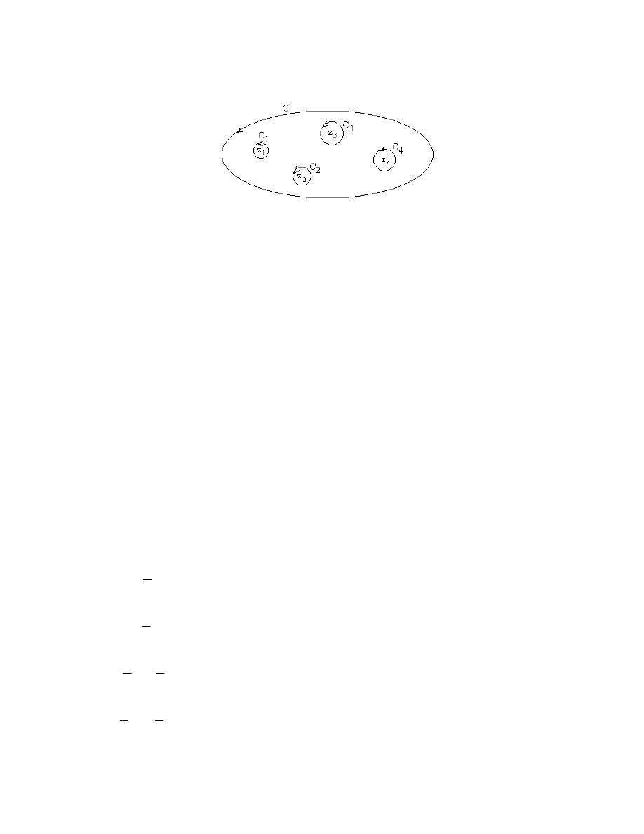
Then,
C
f
zdz
C
1
f
zdz
C
2
f
zdz
C
n
f
zdz
2i
z
z
1
Res f
2i
z
z
2
Res f
2i
z
z
n
Res f
2i
k
1
n
z
z
k
Res f.
This is the celebrated Residue Theorem. It says that the integral of f is simply 2
i times
the sum of the residues at the singular points enclosed by the contour C.
Exercises
Evaluate the integrals. In each case, C is the positively oriented circle |z|
2.
1.
C
e
1/z
2
dz.
2.
C
sin
1
z
dz.
3.
C
cos
1
z
dz.
4.
C
1
z
sin
1
z
dz.
5.
C
1
z
cos
1
z
dz.
10.3
10.2. Poles and other singularities. In order for the Residue Theorem to be of much help
in evaluating integrals, there needs to be some better way of computing the
residue—finding the Laurent expansion about each isolated singular point is a chore. We
shall now see that in the case of a special but commonly occurring type of singularity the
residue is easy to find. Suppose z
0
is an isolated singularity of f and suppose that the
Laurent series of f at z
0
contains only a finite number of terms involving negative powers
of z
z
0
. Thus,
f
z
c
n
z z
0
n
c
n1
z z
0
n
1
c
1
z z
0
c
0
c
1
z z
0
.
Multiply this expression by
z z
0
n
:
z z z
0
n
f
z c
n
c
n1
z z
0
c
1
z z
0
n
1
.
What we see is the Taylor series at z
0
for the function
z z z
0
n
f
z. The coefficient
of
z z
0
n
1
is what we seek, and we know that this is
n1
z
0
n 1!
.
The sought after residue c
1
is thus
c
1
z
z
0
Res f
n1
z
0
n 1!
,
where
z z z
0
n
f
z.
Example
We shall find all the residues of the function
f
z
e
z
z
2
z
2
1
.
First, observe that f has isolated singularities at 0, and
i. Let’s see about the residue at 0.
Here we have
10.4
z z
2
f
z
e
z
z
2
1
.
The residue is simply
0 :
z z
2
1e
z
2ze
z
z
2
1
2
.
Hence,
z
0
Res f
0 1.
Next, let’s see what we have at z
i:
z z ifz
e
z
z
2
z i
,
and so
z
i
Res f
z i e
i
2i
.
In the same way, we see that
z
i
Res f
e
i
2i
.
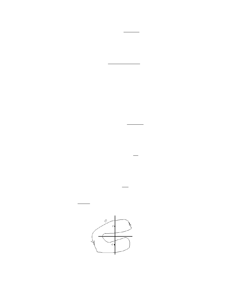
Let’s find the integral
C
e
z
z
2
z
2
1
dz , where C is the contour pictured:
10.5
This is now easy. The contour is positive oriented and encloses two singularities of f; viz, i
and
i. Hence,
C
e
z
z
2
z
2
1
dz
2i
z
i
Res f
z
i
Res f
2i e
i
2i
e
i
2i
2i sin 1.
Miraculously easy!
There is some jargon that goes with all this. An isolated singular point z
0
of f such that the
Laurent series at z
0
includes only a finite number of terms involving negative powers of
z
z
0
is called a pole. Thus, if z
0
is a pole, there is an integer n so that
z z z
0
n
f
z
is analytic at z
0
, and f
z
0
0. The number n is called the order of the pole. Thus, in the
preceding example, 0 is a pole of order 2, while i and
i are poles of order 1. (A pole of
order 1 is frequently called a simple pole.) We must hedge just a bit here. If z
0
is an
isolated singularity of f and there are no Laurent series terms involving negative powers of
z
z
0
, then we say z
0
is a removable singularity.
Example
Let
f
z sin z
z ;
then the singularity z
0 is a removable singularity:
f
z 1z sinz 1z z z
3
3!
z
5
5!
1 z
2
3!
z
4
5!
and we see that in some sense f is ”really” analytic at z
0 if we would just define it to be
the right thing there.
A singularity that is neither a pole or removable is called an essential singularity.
Let’s look at one more labor-saving trick—or technique, if you prefer. Suppose f is a
function:
10.6
f
z
p
z
q
z
,
where p and q are analytic at z
0
, and we have q
z
0
0, while q
z
0
0, and pz
0
0.
Then
f
z
p
z
q
z
p
z
0
p
z
0
z z
0
q
z
0
z z
0
q
z
0
2
z z
0
2
,
and so
z z z
0
fz
p
z
0
p
z
0
z z
0
q
z
0
q
z
0
2
z z
0
.
Thus z
0
is a simple pole and
z
z
0
Res f
z
0
p
z
0
q
z
0
.
Example
Find the integral
C
cos z
e
z
1
dz,
where C is the rectangle with sides x
1, y , and y 3.
The singularities of the integrand are all the places at which e
z
1, or in other words, the
points z
0, 2i, 4i, . The singularities enclosed by C are 0 and 2i. Thus,
C
cos z
e
z
1
dz
2i
z
0
Res f
z
2i
Res f ,
where
f
z cos z
e
z
1
.
10.7
Observe this is precisely the situation just discussed: f
z
p
z
q
z
, where p and q are
analytic, etc.,etc. Now,
p
z
q
z
cos z
e
z
.
Thus,
z
0
Res f
cos 0
1
1, and
z
2i
Res f
cos 2i
e
2
i
e
2
e
2
2
cosh 2.
Finally,
C
cos z
e
z
1
dz
2i
z
0
Res f
z
2i
Res f
2i1 cosh 2
Exercises
6. Suppose f has an isolated singularity at z
0
. Then, of course, the derivative f
also has an
isolated singularity at z
0
. Find the residue
z
z
0
Res f
.
7. Given an example of a function f with a simple pole at z
0
such that
z
z
0
Res f
0, or explain
carefully why there is no such function.
8. Given an example of a function f with a pole of order 2 at z
0
such that
z
z
0
Res f
0, or
explain carefully why there is no such function.
9. Suppose g is analytic and has a zero of order n at z
0
(That is, g
z z z
0
n
h
z, where
h
z
0
0.). Show that the function f given by
f
z
1
g
z
10.8
has a pole of order n at z
0
. What is
z
z
0
Res f ?
10. Suppose g is analytic and has a zero of order n at z
0
. Show that the function f given by
f
z
g
z
g
z
has a simple pole at z
0
, and
z
z
0
Res f
n.
11. Find
C
cos z
z
2
4
dz,
where C is the positively oriented circle |z|
6.
12. Find
C
tan zdz,
where C is the positively oriented circle |z|
2.
13. Find
C
1
z
2
z 1
dz,
where C is the positively oriented circle |z|
10.
10.9
Wyszukiwarka
Podobne podstrony:
Ch10 Q3
ch10
Ch10 E2
Ch10 Q1
BW ch10
Ch10 Q5
ch10 012604
ch10
ch10
Ch10 Placed Features
Ch10 Standard Parts
Ch10 E3
ch10, Sieci Komputerowe Cisco
Ch10 NuclearPowerPlant
cisco2 ch10 focus SL24PPCZXC45HY33A2JRSIZJD3UAHAWWEJ7R7RY
CH10
Ch10
Ch10 Q4
Ch10 E1
więcej podobnych podstron